Wind-optimal lateral trajectories for a multirotor aircraft in urban air mobility

The primary motivation for this paper is to quantify the operational benefits (energy consumption and flight duration) of flying wind-optimal lateral trajectories for short flights (less than 60 miles) anticipated in the urban environment. The optimal control model presented includes a wind model for quantifying the effect of wind on the lateral trajectory. The optimal control problem is numerically solved using the direct collocation method. Energy consumption and flight duration flying wind-optimal lateral trajectories are compared with corresponding values obtained flying great-circle paths between the same origin and destination pairs to determine the operational benefits of wind-optimal routing for short flights. The flight duration results for different scenarios are validated using a simulation tool designed and developed at NASA for exploring advanced air traffic management concepts. This research study suggests that for short flights in an urban environment, operational benefits of the wind-optimal lateral trajectories over the corresponding great-circle trajectories in terms of energy consumption and flight duration per flight are dependent on: i) wind field’s spatial variability, ii) wind magnitude, iii) the direction of route relative to the wind field, and iv) cruise segment length. The operational benefits observed in realistic flyable wind scenarios are less than 2.5%; these could be translated to an equivalent of a maximum of 2 min of cruise flight duration savings in the urban air mobility environment. As expected, headwinds and tailwinds along the flight route most significantly impact energy consumption and flight duration.

1 Introduction

Urban Air Mobility (UAM) can alleviate transportation congestion on the ground by utilizing three-dimensional (3D) airspace efficiently, just as skyscrapers allowed cities to use limited land more efficiently (Uber-Elevate, 2019). The envisioned concept of UAM involves a network of small electric aircraft that can enable rapid and reliable transportation between suburbs and cities and, ultimately, within cities (Thipphavong et al., 2018; Pradeep, 2019; Pradeep and Wei, 2019; Uber-Elevate, 2019).

Recently, technological advances have made it possible to build and flight test eVTOL aircraft (Bosson and Lauderdale, 2018; Thipphavong et al., 2018; Pradeep and Wei, 2019). Several companies, for example, Airbus A³, Aurora Flight Sciences, EHang, Joby Aviation, Kitty Hawk, Leonardo, Lilium, Terrafugia, and Volocopter, are pursuing different design approaches to make eVTOLs a reality (Thipphavong et al., 2018). Despite various designs, they all have distributed electric propulsion (DEP) systems in common (Pradeep and Wei, 2019). However, the low specific energy and nonlinear discharge behavior of current lithium-ion polymer (Li-Po) battery technology used in DEP impose constraints on the flight endurance of such aircraft (Bole et al., 2014). In general, multirotor eVTOLs are a relatively low cruise speed aircraft compared to winged eVTOL aircraft; therefore, atmospheric winds play a significant role in their trajectories. The operational benefits of wind-optimal lateral trajectories have been extensively studied for commercial aircraft (Ng et al., 2012; Sridhar et al., 2014; Sridhar et al., 2015) but not for eVTOLs in the UAM environment. Therefore, in the current research, the operational benefits of wind-optimal lateral trajectories are studied in the UAM context.

The focus of the current research is on the trajectories of a multirotor eVTOL aircraft on short UAM missions (less than 60 miles) (Uber-Elevate, 2019; Uber Air Vehicle Requirements and Missions, 2020). Therefore, an optimal control model for a multirotor eVTOL is formulated that includes a wind effect model to quantify the effect of wind on the trajectory. The optimal control problem formulated using a lateral dynamics model and operational constraints, is numerically solved using the direct collocation method. The primary motivation of the paper is to quantify the operational benefits using wind-optimal lateral trajectories for short flights (less than 60 miles) anticipated in the urban environment. Energy consumption and flight duration flying wind-optimal lateral trajectories in the Dallas-Fort Worth and New York metropolitan areas are compared with the corresponding values obtained flying great-circle paths between the same origin and destination pairs to determine operational benefits of wind-optimal routing for short flights.

In this research, the concept of operations (CONOPs) of the multirotor eVTOL aircraft is assumed to be as follows: i) vertical climb; ii) cruise at a constant altitude along a path between UAM vertiports in metropolitan areas like Dallas-Fort Worth (DFW) and New York (NY); and iii) vertical descent. The scope of this research is focused on the low-altitude (1,600 ft above mean sea level (MSL)) cruise phase (Verma et al., 2020); therefore, climb and descent phases have been ignored in the problem formulation.

The rest of the paper is organized as follows. In Section 2, the optimal control problem with energy consumption as the performance index is formulated to generate four-dimensional (4D) trajectories for a multirotor eVTOL aircraft. The optimal control model presented includes a wind model for quantifying the effect of wind on a lateral trajectory. In Section 3, wind-optimal and great-circle lateral trajectories generated under different wind conditions are described. Next, the flight duration results for different scenarios are validated using the simulation tool designed and developed at NASA. Finally, the main findings for this study are summarized in Section 4.

2 Optimal control model

2.1 eVTOL aircraft model

In this research, a quadrotor eVTOL aircraft concept proposed by Silva et al. (2018), as shown in Figure 1A, is used to study the effect of wind on a multirotor eVTOL aircraft trajectory. This eVTOL has six-seater (up to 545 kg payload) capacity with a long range cruise airspeed (LRC) of 50.4 m/s (98 kts).

FIGURE 1

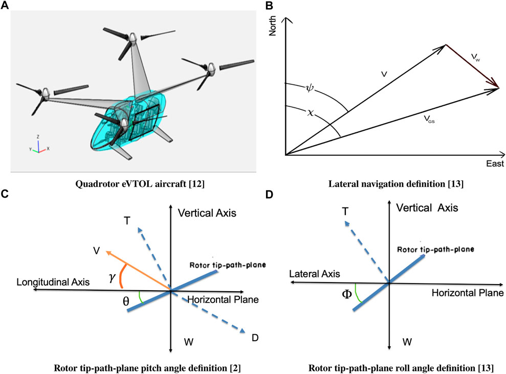
FIGURE 1. Multirotor eVTOL aircraft in forward flight.

Table 1 lists the aircraft performance data for the lateral trajectory optimization in cruise phase.

TABLE 1

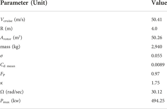
TABLE 1. Performance data of the eVTOL aircraft (Silva et al., 2018).

2.2 Flight dynamics and kinematics model

To study the effect of wind on the cruise phase of the multirotor eVTOL aircraft, a lateral flight dynamics model (two dimensional in space and one dimensional in time) is considered. The four lateral states of the model are: λ, τ, V, ψ; where λ is the latitude, τ is the longitude, V is the true airspeed (assumed to have only horizontal component during the cruise) and ψ is the heading angle w. r.t north (Tsuchiya et al., 2009; Yomchinda et al., 2011). The three control variables of the model are: the net thrust (T), the rotor tip-path-plane pitch angle (θ) and the rotor tip-path-plane roll (bank) angle (ϕ). Therefore, the quasi-steady cruise flight dynamics and kinematics of the multirotor eVTOL aircraft considering wind in a vehicle-carried frame of reference are as follows (Erzberger and Lee, 1980; Tsuchiya et al., 2009; Yomchinda et al., 2011; Sridhar et al., 2015; Weitz, 2015; Pradeep, 2019; Pradeep and Wei, 2019):

$\frac{dV}{dt}=\frac{T\mathit{cos}\varphi \mathit{sin}\theta -D}{m}-\frac{d{W}_N}{dt}\mathit{cos}\psi -\frac{d{W}_E}{dt}\mathit{sin}\psi (1)$

$V\frac{d\psi }{dt}=\frac{T\mathit{sin}\varphi }{m}+\frac{d{W}_N}{dt}\mathit{sin}\psi -\frac{d{W}_E}{dt}\mathit{cos}\psi (2)$

$\left(R_{\text{Earth}}+h\right)\frac{d\lambda }{dt}=V\mathit{cos}\psi +W_N=V_{GS}\mathit{cos}\chi (3)$

$\left(R_{\text{Earth}}+h\right)\mathit{cos}\lambda \frac{d\tau }{dt}=V\mathit{sin}\psi +W_E=V_{GS}\mathit{sin}\chi (4)$

where D is the parasite drag, V_GS is the ground speed, χ is the course, h is the altitude above mean sea level and R_Earth is the mean radius of the Earth, and W_N and W_E are the components of the wind in north and east directions, respectively. The time derivative of wind components is assumed to be zero given the short duration flights in the UAM environment (Thipphavong et al., 2018; Uber-Elevate, 2019).

For the quadrotor eVTOL aircraft, assuming that the rotors have negligible interference with each other, the net thrust (T) produced by the four rotors is given by:

$T=\sum _{n=1}^4{\left(T_{\text{rotor}}\right)}_n(5)$

where ${(T_{\text{rotor}})}_n$ is the thrust produced by the nth rotor. Also, assuming all the rotors produce the same amount of thrust (T_rotor) in cruise phase, the net thrust (T) produced by the rotors is given by:

$T=4T_{\text{rotor}}(6)$

2.3 Drag model

The parasite drag (D) on the multirotor eVTOL is calculated as follows (Silva et al., 2018):

$D=1.1984\frac{\rho V^2}{2}(7)$

where ρ is the density of air, which is a function of altitude and 1.1984 is a product of drag coefficient and reference area (Silva et al., 2018).

2.4 Induced velocity and induced power

Using momentum theory (Heyson, 1975; Hoffmann et al., 2007; Johnson, 2012), the hover induced velocity (v_h) is given by:

$v_h=\sqrt{\frac{T_{\text{rotor}}}{2\rho A_{\text{rotor}}}}(8)$

where A_rotor is the rotor diVsk area (πR²) and R is the radius of the rotor.

Consider an isolated rotor in forward motion at true airspeed (V), with angle of attack (α) between the air-stream and the rotor disk (tip-path-plane). Using momentum theory in forward flight, the solution for induced velocity (v_i) is given by (Heyson, 1975; Hoffmann et al., 2007; Johnson, 2012):

$v_i=\frac{v_h^2}{\sqrt{{\left(V\mathit{cos}\alpha \right)}^2+{\left(V\mathit{sin}\alpha +v_i\right)}^2}}(9)$

where the hover induced velocity (v_h) on the right-hand side of Eq. 9 is computed using Equation 8.

Equation 9 is a quartic polynomial that can be analytically solved for induced velocity (v_i). Out of the four roots of the quartic Eq. 9, the one with real-positive and value lower than v_h is the correct solution for cruise phase. Equation 9 can also be numerically solved using an iterative technique with initial guess for v_i as v_h.

Once v_i is computed, the induced power loss of an isolated rotor (P_{induced rotor}) in forward flight is computed as follows (Johnson, 2012; Johnson, 2015):

$P_{\text{induced\hspace{0.17em}rotor}}=\kappa T_{\text{rotor}}{v}_i(10)$

where the induced power factor (κ) is assumed to be 1.75 (Silva et al., 2018).

2.5 Power required by the eVTOL aircraft

Based on the quasi-steady flight assumption, the instantaneous power required in forward cruise flight at a constant altitude is equal to the sum of the induced power, parasite power, and profile power as follows (Heyson, 1975; Leishman, 2002; Johnson, 2012; Pradeep, 2019; Pradeep and Wei, 2019):

$P_{\text{required}}=P_{\text{induced}}+P_{\text{parasite}}+P_{\text{profile}}(11)$

The total induced power loss of the eVTOL aircraft (P_induced) is equal to the summation of the induced power loss of each rotor (P_{induced rotor}). Therefore, the induced power loss of the aircraft is given by Johnson (2012); Silva et al. (2018):

$P_{\text{induced}}=\sum _{n=1}^4{\left(P_{\text{induced\hspace{0.17em}rotor}}\right)}_n=\kappa \sum _{n=1}^4{\left(T_{\text{rotor}}\right)}_n{\left(v_i\right)}_n(12)$

The power required to propel the aircraft forward (the parasite power loss) at a constant altitude is given by Johnson (2012):

$P_{\text{parasite}}=TV\mathit{sin}\alpha (13)$

The profile power loss is calculated from a mean blade drag coefficient (C_{d mean}) as follows (Leishman, 2002; Johnson, 2012; Silva et al., 2018):

$P_{\text{profile}}=\frac{\rho A_{\text{rotor}}{\left(\mathrm{\Omega }R\right)}^3\sigma C_{dmean}{F}_P}{8}(14)$

where Ω is the rotational velocity of the rotor blades, σ is the thrust weighted solidity ratio, C_{d mean} is the mean blade drag coefficient and F_P is the function that accounts for the increase of the blade section velocity with rotor edgewise and axial speed (Johnson, 2012; Johnson et al., 2018; Silva et al., 2018). However, F_P is assumed to be a constant (see Table 1) in this study because of cruise at constant altitude and nominal cruise speed.

Therefore, using the equations from (11) to (14), the instantaneous power required (P_required) in forward flight is given by:

$P_{\text{required}}=\kappa \sum _{n=1}^4{\left(T_{\text{rotor}}\right)}_n{\left(v_i\right)}_n+TV\mathit{sin}\alpha +\frac{\rho A_{\text{rotor}}{\left(\mathrm{\Omega }R\right)}^3\sigma C_{dmean}{F}_P}{8}(15)$

2.6 Performance index of optimal control problem

The performance index for the wind-optimal lateral trajectory optimization problem is constructed as follows:

$\begin{array}{ll}\hfill J& ={\mathit{\int }}_{t_0}^{t_f}\left(P_{\text{required}}\right)dt\hfill \\ \hfill & ={\mathit{\int }}_{t_0}^{t_f}\left(\kappa \sum _{n=1}^4{\left(T_{\text{rotor}}\right)}_n{\left(v_i\right)}_n+TV\mathit{sin}\alpha +\frac{\rho A_{\text{rotor}}{\left(\mathrm{\Omega }R\right)}^3\sigma C_{dmean}{F}_P}{8}\right)dt\hfill \end{array}(16)$

where t₀ is the initial flight time at the top of climb (TOC) placed directly above the origin vertiport at the cruise altitude and t_f is the final flight time to reach the top of descent (TOD) placed directly above the destination vertiport at the cruise altitude.

2.7 Path constraints of optimal control problem

For a level flight (cruise) in the absence of vertical component of wind, the net vertical force on the multirotor eVTOL aircraft is zero; therefore, the following path constraint is imposed on the problem:

$T\mathit{cos}\varphi \mathit{cos}\theta =mg(17)$

where m is the mass of the aircraft and g is the acceleration due to gravity.

The instantaneous power required (P_required in kw) is bounded by the total deliverable power (P_max) of the quadrotor eVTOL aircraft (Johnson, 2015; Silva et al., 2018):

$P_{\text{required}}\le 494.25(18)$

where P_required is defined in Equation 15.

2.8 Great-circle path constraint

The course angle (χ) for the great-circle trajectory between the two waypoints is calculated as follows (Chatterji et al., 1996):

$\mathit{tan}\chi =\frac{\mathit{sin}\left({\tau }_2-{\tau }_1\right)\mathit{cos}{\lambda }_2}{\mathit{sin}{\lambda }_2\mathit{cos}{\lambda }_1-\mathit{sin}{\lambda }_1\mathit{cos}{\lambda }_2\mathit{cos}\left({\tau }_2-{\tau }_1\right)}(19)$

where the origin latitude-longitude is (λ₁, τ₁) and the destination latitude-longitude is (λ₂, τ₂). However, to generate a great-circle trajectory between the two waypoints using the optimal control framework developed in this research, a path constraint as a function of the wind components (W_N and W_E), latitude-longitude coordinates of the two waypoints and heading angle (ψ) is required. Therefore, the course angle (χ) needs to be eliminated from Equation 19.

Using Eqs 3, 4, the heading angle (ψ) required to fly the course angle (χ) in the presence of the wind is computed as follows:

$\mathit{tan}\chi =\frac{Vsin\psi +W_E}{Vcos\psi +W_N}(20)$

where W_N and W_E are the components of the wind in north and east directions, respectively.

Equations 19, 20 result in the following relation:

$\frac{Vsin\psi +W_E}{Vcos\psi +W_N}=\frac{\mathit{sin}\left({\tau }_2-{\tau }_1\right)\mathit{cos}{\lambda }_2}{\mathit{sin}{\lambda }_2\mathit{cos}{\lambda }_1-\mathit{sin}{\lambda }_1\mathit{cos}{\lambda }_2\mathit{cos}\left({\tau }_2-{\tau }_1\right)}(21)$

Hence, the path constraint for the great-circle trajectory between the two waypoints is given by:

$\left(Vsin\psi +W_E\right)\left(\mathit{sin}{\lambda }_2\mathit{cos}{\lambda }_1-\mathit{sin}{\lambda }_1\mathit{cos}{\lambda }_2\mathit{cos}\left({\tau }_2-{\tau }_1\right)\right)-\left(Vcos\psi +W_N\right)\left(\mathit{sin}\left({\tau }_2-{\tau }_1\right)\mathit{cos}{\lambda }_2\right)=0(22)$

3 Numerical study and results

3.1 Optimal control solver

The trajectory optimization problems can be numerically solved, either using the direct or indirect methods (Betts and Huffman, 1998). Direct methods typically discretize the trajectory optimization problem, and convert the original trajectory optimization problem into a nonlinear program. On the other hand, indirect methods are characterized by explicitly solving the optimality conditions stated in terms of the adjoint differential equations, the maximum principle, and associated boundary (transversality) conditions (Bryson, 1975). Using the calculus of variations, the optimal control necessary conditions can be derived by setting the first variation of the Hamiltonian function to zero. A common way to distinguish these two methods is that a direct method discretizes and then optimizes, while an indirect method optimizes and then discretizes (Betts and Huffman, 1998; Kelly, 2017).

In this research, PSOPT has been used to solve the optimal control problem to generate wind-optimal lateral trajectories for the multirotor eVTOL aircraft. PSOPT is an open-source optimal control software package written in C++ that uses direct collocation methods such as pseudospectral methods (Becerra, 2010). Pseudospectral methods directly discretize the original optimal control problem to formulate a nonlinear programming problem, which is then solved numerically using a sparse nonlinear programming solver to find approximate local optimal solutions. IPOPT is an open-source C++ package for large-scale nonlinear optimization, which uses an interior point method (Wächter and Biegler, 2006; Becerra, 2010). IPOPT is the default nonlinear programming algorithm used by PSOPT. Approximation theory and practice show that pseudospectral methods are well suited for approximating smooth functions, integration, and differentiation, i.e., all of which are relevant to optimal control problems (Becerra, 2010). Nearly all trajectory optimization techniques require a good initial guess to begin the optimization. In the best case, a good initialization ensures that the solver rapidly arrives at the optimal solution (Kelly, 2017).

3.2 Wind data

The Rapid Refresh (RR) operational weather prediction system, available on an hourly basis at 13 km spatial resolution from the National Center for Environmental Prediction (Benjamin et al., 1998), has been used to extract the wind data for analysis. The wind data are extracted for the entire month of January 2019 (i.e., 31 days) during peak traffic hours in the morning and evening, i.e., i) 7 a.m.–11 a.m. (local time), and ii) 3 p.m.–7 p.m. (local time) at cruise altitude (1,600 ft above MSL) in 1-min intervals at grid points equispaced 10 km apart. The grid points cover 10⁴ km² area at the Dallas-Fort Worth and New York metropolitan areas of the United States.

3.2.1 Strongest wind

To find the date and local time when the strongest wind (highest wind speed) occurred: First, the spatial average of wind speed is computed in 1-min intervals (epochs). Finally, the spatially averaged wind speeds at each epoch are compared to find the epoch at which the highest wind speed magnitude occurred.

3.2.2 Highest spatial variability of the wind

To find the date and local time when the highest spatial variability of wind speed occurred: First, the spatial average of wind speed is computed in 1-min intervals (epochs). Next, the standard deviation of the wind is computed in 1-min intervals as follows:

${\sigma }_{\mathit{wind}}=\sqrt{{\sigma }_{W_N}^2+{\sigma }_{W_E}^2}(23)$

where σ_wind is the standard deviation of the wind at any given epoch, ${\sigma }_{W_N}$ is the standard deviation of the north component of the wind at any given epoch, and ${\sigma }_{W_E}$ is the standard deviation of the east component of the wind at any given epoch. Finally, the standard deviation of the wind at each epoch is compared to find the epoch at which the highest spatial variability occurred.

3.2.3 Wind data analysis results

Table 2 and Table 3 show the following wind data analysis results:

• Date and time results in epoch, UTC, and local time format for the occurrence of the strongest wind and highest spatial variability of the wind in the Dallas-Fort Worth (DFW) and New York (NY) metropolitan areas.

• Statistics of wind fields chosen for the study in the Dallas-Fort Worth and New York metropolitan areas respectively.

TABLE 2

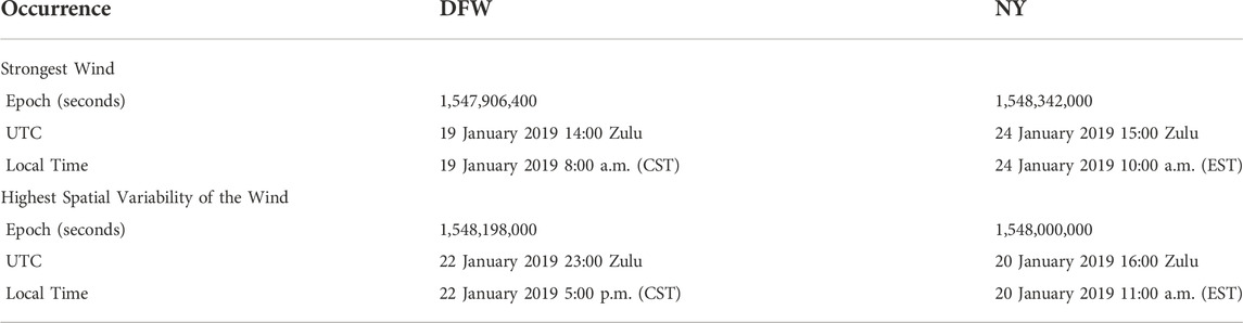
TABLE 2. Occurrence of the strongest wind and highest spatial variability of the wind in the Dallas-Fort Worth (DFW) and the New York (NY) metropolitan areas.

TABLE 3

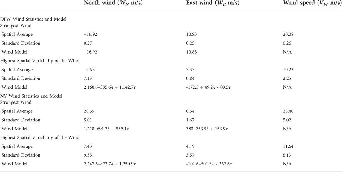
TABLE 3. Wind statistics and model of the strongest wind and highest spatial variability of the wind in the Dallas-Fort Worth (DFW) and the New York (NY) metropolitan areas.

3.2.4 Analytical wind models for case studies

Because PSOPT requires the equations in an analytical form, the MATLAB curve-fitting Toolbox (2001) is used to obtain equations for north and east components of the wind, needed in Eqs 3, 4 for each case study. These equations are approximation of real wind data as a linear function of latitude (λ) and longitude (τ), defined in radians.

Table 3 shows wind models obtained using MATLAB Toolbox (2001) for different wind scenarios in the DFW and NY metropolitan areas. In general, R-square is a goodness-of-fit measure for linear regression models. R-square measures the strength of the relationship between the linear regression model and the dependent variable on a convenient 0 to 1 scale (Toolbox, 2001). For the four wind models shown in Table 3, R-square values are observed between 0.91 and 0.95.

3.3 Test apparatus

NASA’s Future Air Traffic Management (ATM) Concepts Evaluation Tool (FACET), designed and developed over the last 20 years, provides a flexible simulation environment for the exploration, development and evaluation of advanced ATM concepts (Bilimoria et al., 2001). FACET models four-dimensional (4D) aircraft trajectories in the presence of winds using round-earth kinematic equations. Aircraft can be flown along flight plan routes or great-circle routes as they climb, cruise and descend per their aircraft-type performance models. Performance parameters of the aircraft are obtained from a data look-up table. Therefore, a look-up table is created for the multirotor eVTOL aircraft based on the performance data of the conceptual multirotor eVTOL proposed by Silva et al. (2018). The flight duration results of the optimal control framework using PSOPT solver are validated using the neighboring-optimal wind routing algorithm (Jardin and Bryson, 2001) implemented in FACET. FACET implementation performs a bi-linear interpolation in spatial and temporal dimensions on the available gridded wind data.

3.4 Metrics to measure operational benefits

The following two metrics are used to compute operational benefits of flying wind-optimal lateral trajectory compared to great-circle trajectory for a given origin and destination.

3.4.1 Energy savings

The energy savings (%) associated with flying the wind-optimal lateral trajectory compared to the great-circle trajectory is computed as follows:

$\text{Energy\hspace{0.17em}Savings\hspace{0.17em}}\left(\text{\%}\right)=\frac{{\text{Energy}}_{\text{Great}-\text{Circle}}-{\text{Energy}}_{\text{Wind}-\text{Optimal}}}{{\text{Energy}}_{\text{Great}-\text{Circle}}}100(24)$

where Energy_Wind-Optimal and Energy_Great-Circle are energy consumed flying the wind-optimal lateral trajectory and great-circle trajectory under similar wind conditions, respectively.

3.4.2 Flight duration savings

The flight duration savings (%) associated with flying the wind-optimal lateral trajectory compared to the great-circle trajectory is computed as follows:

$\text{Flight\hspace{0.17em}Duration\hspace{0.17em}Savings\hspace{0.17em}}\left(\text{\%}\right)=\frac{{\text{Flight\hspace{0.17em}Duration}}_{\text{Great}-\text{Circle}}-{\text{Flight\hspace{0.17em}Duration}}_{\text{Wind}-\text{Optimal}}}{{\text{Flight\hspace{0.17em}Duration}}_{\text{Great}-\text{Circle}}}100(25)$

where Flight Duration_Wind-Optimal and Flight Duration_Great-Circle are flight duration flying the wind-optimal lateral trajectory and great-circle trajectory under same wind conditions, respectively.

3.4.3 Dallas-Fort Worth metropolitan area

Two types of wind scenarios are considered: i) strongest wind (as shown in Figure 2) and ii) highest spatial variability of the wind (Figure 4) in the Dallas-Fort metropolitan area. The location of vertiports and the direct route lengths are based on the Air Traffic Management - eXploration (ATM-X), Urban Air Mobility (UAM) Experiment two scenarios conducted at NASA Ames (Verma et al., 2020). Therefore, the great-circle distance between different origin and destination pairs is 30–50 nautical miles.

FIGURE 2

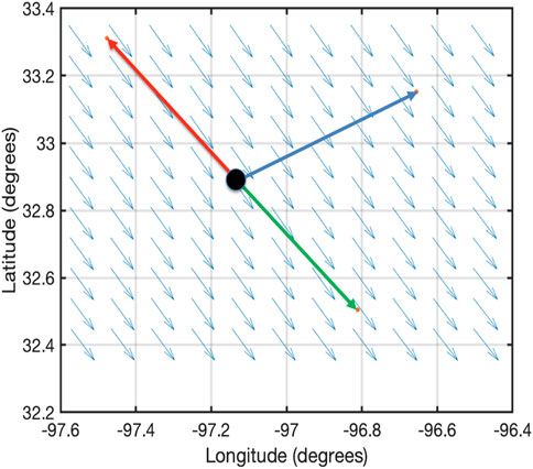
FIGURE 2. Depiction of wind field and routes used to study operational benefits of flying wind-optimal lateral trajectories in the DFW metropolitan area for the strongest wind case study.

3.4.4 Case study - Strongest wind in the Dallas-Fort Worth metropolitan area

To study wind-optimal lateral trajectories, three routes originating from the origin location (32.901767, -97.193954) are considered (Verma et al., 2020). The destinations are chosen at a great-circle distance of 30 nautical miles from the origin. Figure 2 shows a depiction of wind fields and routes used to study the operational benefits of flying wind-optimal lateral trajectories in the Dallas-Fort Worth metropolitan area for the strongest-wind (Table 3) case study.

From Figure 3, it can be seen that in the uniform wind field, the energy consumption and flight duration for the wind-optimal lateral trajectories are the same as the corresponding great-circle trajectories. However, because of the slow nominal cruise speed (50.41 m/s), the energy consumption and flight duration while flying in the headwind is 2–3 times higher than flying the same distance (30 nm) in the tailwind. As shown in Figure 3, the flight duration (cruise) results of PSOPT are validated using the overall flight duration (climb, cruise, and descent) results of FACET. The flight duration results obtained using FACET are generally slightly different (1–2 min) because of: i) climb and descent phases modeled in FACET, which are not considered in PSOPT; and ii) slight difference in the wind field modeling between FACET and PSOPT. FACET directly uses rapid refresh wind data at grid points for trajectory prediction, whereas PSOPT uses a wind model created using Matlab curve-fitting toolbox.

FIGURE 3

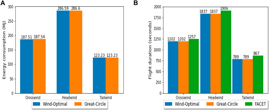
FIGURE 3. Comparison of wind-optimal and great-circle trajectories under different wind conditions in the Dallas-Fort Worth metropolitan area for the strongest wind case study.

3.4.5 Case study - Highest spatial variability of wind in the Dallas-Fort Worth metropolitan area

To study the impact of spatial variability of the wind field on the wind-optimal lateral trajectory, two routes (50 nm great-circle distance) as shown in Figure 4 are considered. The wind model used to generate wind-optimal and great-circle trajectories is listed in Table 3.

FIGURE 4

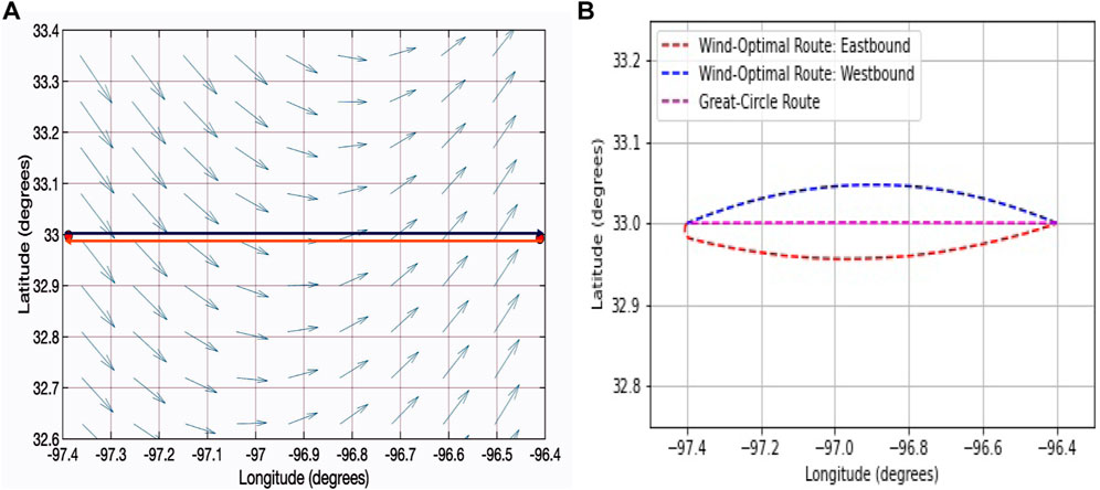
FIGURE 4. Depiction of wind field, routes and computed wind-optimal lateral trajectories used to study operational benefits of flying wind-optimal lateral trajectories in the DFW metropolitan area for the highest spatial variability of the wind case study.

In this case study, the operational benefits (energy consumption and flight duration) with the wind-optimal lateral trajectory when compared to the corresponding great-circle trajectory are observed to be slightly less than 1% for both the routes as shown in Figure 5. From Figure 5, it can be concluded that the spatial variability of the wind field has an impact on the amount of operational benefits.

FIGURE 5

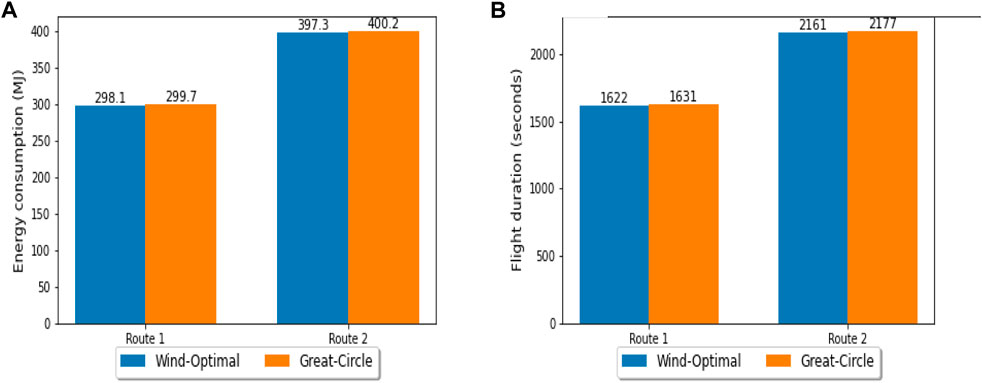
FIGURE 5. Comparison of wind-optimal lateral trajectory with great-circle trajectory in the DFW metropolitan area for the highest spatial variability of the wind case study.

3.5 New York metropolitan area

Similar to the Dallas-Fort Worth case studies, two types of wind scenarios are considered: 1) strongest wind (as shown in Figure 6) and ii) highest spatial variability of the wind (as shown in Figure 8) in the New York metropolitan area. The vertiports and direct route lengths of 30 and 50 nautical miles are based on the Air Traffic Management - eXploration (ATM-X), Urban Air Mobility (UAM) Experiment two conducted at NASA Ames (Verma et al., 2020).

FIGURE 6

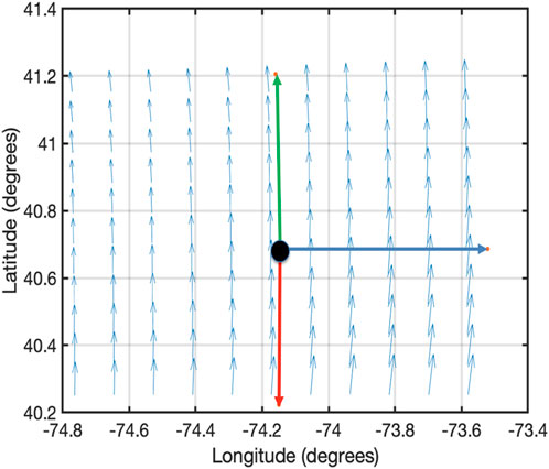
FIGURE 6. Depiction of wind field and routes used to study operational benefits of flying wind-optimal lateral trajectories in the New York metropolitan area for the strongest wind case study.

3.5.1 Case study - Strongest wind in the New York metropolitan area

To study wind-optimal lateral trajectories, three routes originating from the location (40.703869, -74.176071) as shown in Figure 6 are considered.

From Figure 7, it can be seen that in the non-uniform wind field, the energy consumption and flight duration for the wind-optimal lateral trajectory are 1.2% lower than the corresponding great-circle trajectory. However, because of the slow nominal cruise speed (50.41 m/s) and high magnitude of the headwind (approx. 28 m/s), the energy consumption and flight duration while flying in the headwind is 4–5 times higher than flying the same distance (30 nm) in the tailwind. As shown in Figure 7, the flight duration (cruise) results of PSOPT are validated using overall flight duration (climb, cruise, and descent) results obtained using FACET. The flight duration results of FACET are generally slightly different (1–2 min) because of: i) climb and descent phases modeled in FACET, which are not considered in PSOPT; and ii) slight difference in the wind field modeling between FACET and PSOPT. FACET directly uses rapid refresh wind data at grid points for trajectory prediction, whereas PSOPT uses a wind model created using Matlab curve-fitting toolbox. Therefore, the slightly lower flight duration (around 1.5%) result obtained using FACET under headwind conditions in Figure 7 can be attributed to a higher contribution from wind modeling error in this scenario.

FIGURE 7

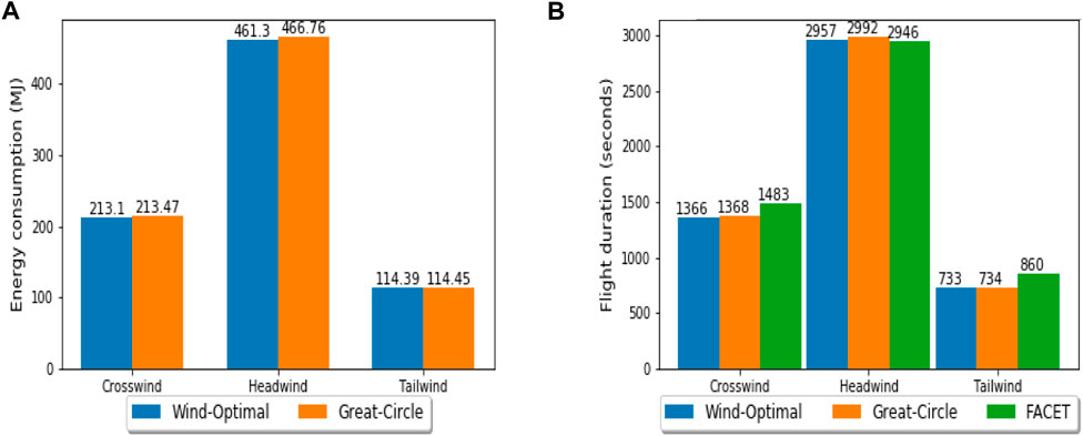
FIGURE 7. Comparison of wind-optimal and great-circle trajectories under different wind conditions in the New York metropolitan area for the strongest wind case study.

To perform the sensitivity analysis on wind-optimal lateral trajectory, the headwind route is further extended to 50 nm (57.54 miles). The headwind route is picked among the three routes because it showed the greatest operational benefits (energy consumption and flight duration) of 1.2% for wind-optimal lateral trajectory when compared to the corresponding great-circle trajectory. For the headwind route (origin: 41.3661, -74.176071 and destination: 40.2, -74.176071), the operational benefits with the wind-optimal lateral trajectory when compared to the great-circle trajectory are approximately 2.5% as listed in Table 4. From Table 4 and Figure 7, it can be concluded that the length of the direct route, spatial variability of the wind field, wind magnitude, and direction of the direct route relative to the wind field impact the percentage of operational benefits.

TABLE 4

TABLE 4. Comparison of wind-optimal lateral trajectory with great-circle trajectory on headwind route (50 nm).

3.5.2 Case study - Highest spatial variability of the wind in the New York metropolitan area

To study the impact of spatial variability of the wind field on the wind-optimal lateral trajectory, two routes (50 nm great-circle distance) as shown in Figure 8.

FIGURE 8

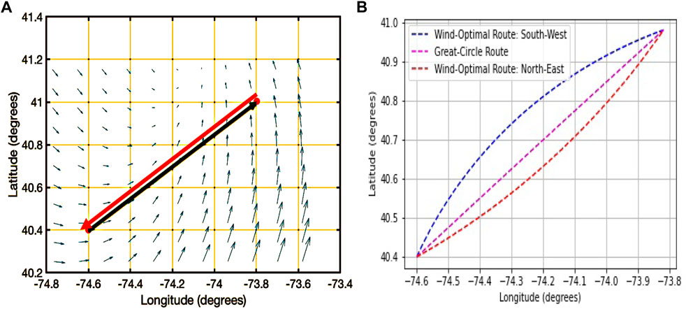
FIGURE 8. Depiction of wind field, routes and computed wind-optimal lateral trajectories used to study operational benefits of flying wind-optimal lateral trajectories in the New York metropolitan for the highest spatial variability of the wind case study.

In this case study, the operational benefits of flying a wind-optimal route compared to the great-circle route for North-East bound flight are approximately 1.1%. However, the operational benefits of flying a wind-optimal route compared to the great-circle route for South-West bound flight are about 2.3% as shown in Figure 9. The results of this case study reiterate the earlier conclusion that the length of the direct route, spatial variability of the wind field, wind magnitude, and direction of the direct route relative to the wind field impact the percentage of operational benefits.

FIGURE 9

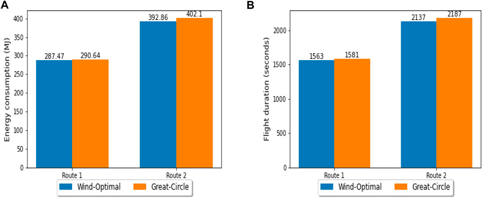
FIGURE 9. Comparison of wind-optimal lateral trajectory with great-circle trajectory in the New York metropolitan area for the highest spatial variability of the wind case study.

3.5.3 Case study - Simulated wind in the Dallas-Fort Worth metropolitan area

Since 50 nm great-circle distance corresponds to 6–7 wind extraction grid points with 13 km resolution for wind data, therefore, wind field is simulated to perform sensitivity analysis and substantiate the results of the impact of wind field with varying direction (higher magnitude of a spatial gradient than previous case studies) on a wind-optimal lateral trajectory. The north component of the wind (W_N) is linearly varied from its maximum magnitude with the direction towards the north at the origin vertiport (32.901767, -97.193954) to its maximum magnitude with the direction towards the south at the destination vertiport (32.897850, -96.204208) as shown in Subfigure 10a. In the simulated wind-field scenario, the north component of the wind (W_N) is linearly varied from +15 m/s at the origin vertiport to - 15 m/s at the destination vertiport as shown in Subfigure 10a, whereas the east component of the wind (W_E) is kept constant.

The linear curve-fit of the north component of the wind (W_N m/s) obtained using the MATLAB curve-fitting tool (Toolbox, 2001) is as follows:

$W_N=-1736.68\tau -2931.03(26)$

$W_E=15(27)$

From Table 5, it can be seen that in the wind field with varying direction as shown in Figure 10, for the multirotor eVTOL aircraft on a short UAM mission (50 nm), the energy consumption and flight duration for the wind-optimal lateral trajectory are approximately 1.4% lower than the corresponding great-circle trajectory.

TABLE 5

TABLE 5. Comparison of wind-optimal lateral trajectory with great-circle trajectory in simulated wind with varying direction.

FIGURE 10

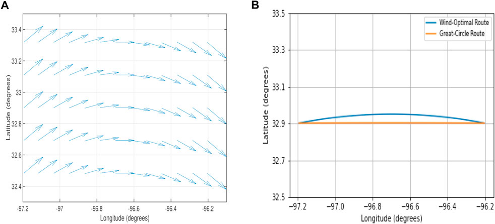
FIGURE 10. Wind-optimal lateral trajectory and great-circle trajectory in simulated wind with varying direction.

4 Conclusion

The optimal control problem with energy consumption as the performance index was formulated to generate trajectories for a multirotor electric vertical takeoff and landing aircraft on a short urban air mobility mission (less than 60 miles). The optimal control model presented includes a wind model for quantifying the effect of wind on the lateral trajectory. The wind models were formulated by analyzing the real wind data from the Rapid Refresh (RR) operational weather prediction system in the Dallas-Fort Worth and New York metropolitan areas for the following scenarios: 1) strongest wind and ii) highest spatial variability of the wind.

Further, this paper presents a framework for comparing energy consumption and flight duration flying wind-optimal lateral trajectories and great-circle trajectories to evaluate the operational benefits (energy consumption and flight duration) of wind-optimal routing for short flights. The lateral trajectory optimization problem was numerically solved using the pseudospectral method for a NASA-proposed conceptual multirotor electric vertical takeoff and landing aircraft.

The numerical results in the Dallas-Fort Worth metropolitan area for the strongest wind case study showed that in uniform wind conditions, the wind-optimal lateral trajectories were identical to the corresponding great-circle trajectories for short flights (30 nm). However, the highest spatial variability of the wind case study showed operational benefits of slightly less than 1% for both of the 50 nm direct routes, i.e., Eastbound and Westbound.

The numerical results in the New York metropolitan area for the strongest wind case study showed operational benefits flying the wind-optimal lateral trajectories compared to the corresponding great-circle trajectories for short flights (30 nm) with maximum benefit (1.2%) in the headwind condition. Upon performing a sensitivity analysis by extending the headwind route to 50 nm, the operational benefits increased to 2.5%. The operational benefits can be attributed to non-uniform wind conditions. However, the highest spatial variability of the wind case study showed operational benefits of 2.3% for the South-West bound 50 nm direct route, and 1.1% for the North-East bound 50 nm direct route.

In conclusion, this research study suggests that for short flights in an urban environment, operational benefits of the wind-optimal lateral trajectories over the corresponding great-circle trajectories in terms of energy consumption and flight duration per flight are dependent on multiple factors. These factors are: 1) wind field’s spatial variability, ii) wind magnitude, iii) the direction of route relative to the wind field, and iv) cruise segment length. The operational benefits observed in realistic flyable wind scenarios are less than 2.5%; these could be translated to an equivalent of a maximum of 2 min of cruise flight duration savings in the urban air mobility environment. As expected, headwinds and tailwinds along the flight route significantly impact energy consumption and flight duration.

Data availability statement

The data analyzed in this study is subject to the following licenses/restrictions: NASA Export Compliance. Requests to access these datasets should be directed to priyank.pradeep@nasa.gov.

Author contributions

PP—Problem Formulation, Problem Solver Using Direct Collocation Method, and Manuscript Documentation GC—Problem Formulation and Discussion of Results TL—Problem Formulation, Discussion of Results, and Technical Lead KS—Validation of Wind-Optimal Trajectories using FACET Tool CL—Wind Data (Rapid Refresher) Provider HE—Guidance on Wind-Optimal Trajectories BS—Guidance on Wind-Optimal Trajectories.

Funding

The material is based upon work supported by NASA under award number NNA16BD14C for NASA Academic Mission Services (NAMS).

Acknowledgments

The authors thank Wayne Johnson, Christopher Silva, Carlos A. Malpica, and Gloria K. Yamauchi from the Aeromechanics branch at NASA Ames Research Center for constructive discussions and their valuable time. Also, special thanks to Christopher Silva for reviewing the drag and power equations. Part of this material was presented as a conference paper at the 2020 AIAA Aviation Forum (Pradeep et al., 2020).

Conflict of interest

GB was employed by Crown Consulting Inc.

The remaining authors declare that the research was conducted in the absence of any commercial or financial relationships that could be construed as a potential conflict of interest.

Publisher’s note

All claims expressed in this article are solely those of the authors and do not necessarily represent those of their affiliated organizations, or those of the publisher, the editors and the reviewers. Any product that may be evaluated in this article, or claim that may be made by its manufacturer, is not guaranteed or endorsed by the publisher.

References

Becerra, V. M. (2010). “Solving complex optimal control problems at no cost with PSOPT,” in 2010 IEEE International Symposium on Computer-Aided Control System Design, 1391–1396. doi:10.1109/CACSD.2010.5612676

CrossRef Full Text | Google Scholar

Benjamin, S. G., Brown, J. M., Brundage, K. J., Schwartz, B. E., Smirnova, T. G., Smith, T. L., et al. (1998). NWS technical procedures bulletin 448 RUC-2-the rapid update cycle version 2.

Google Scholar

Betts, J. T., and Huffman, W. P. (1998). Mesh refinement in direct transcription methods for optimal control. Optim. Control Appl. Methods 19 (1), 1–21. doi:10.1002/(sici)1099-1514(199801/02)19:1<1::aid-oca616>3.0.co;2-q

CrossRef Full Text | Google Scholar

Bilimoria, K. D., Sridhar, B., Grabbe, S. R., Chatterji, G. B., and Sheth, K. S. (2001). Facet: Future ATM concepts evaluation tool. Air Traffic Control Q. 9 (1), 1–20. doi:10.2514/atcq.9.1.1

CrossRef Full Text | Google Scholar

Bole, B., Daigle, M., and Gorospe, G. (2014). Online prediction of battery discharge and estimation of parasitic loads for an electric aircraft. ESC 2, 5S2P.

Google Scholar

Bosson, C., and Lauderdale, T. A. (2018). “Simulation evaluations of an autonomous urban air mobility network management and separation service,” in 2018 Aviation Technology, Integration, and Operations Conference, 3365. doi:10.2514/6.2018-3365

CrossRef Full Text | Google Scholar

Bryson, A. E. (1975). Applied optimal control: Optimization, estimation and control. United Kingdom: CRC Press.

Google Scholar

Chatterji, G., Sridhar, B., and Bilimoria, K. (1996). “En-route flight trajectory prediction for conflict avoidance and traffic management,” in Guidance, Navigation, and Control Conference, 3766.

CrossRef Full Text | Google Scholar

Erzberger, H., and Lee, H. (1980). Constrained optimum trajectories with specified range. J. Guid. Control 3 (1), 78–85. doi:10.2514/3.55950

CrossRef Full Text | Google Scholar

Heyson, H. H. (1975). “A momentum analysis of helicopters and autogyros in inclined descent, with comments on operational restrictions,” 1975.

Google Scholar

Hoffmann, G., Huang, H., Waslander, S., and Tomlin, C. (2007). “Quadrotor helicopter flight dynamics and control: Theory and experiment,” in AIAA Guidance, Navigation and Control Conference and Exhibit, 6461.

CrossRef Full Text | Google Scholar

Jardin, M. R., and Bryson, A. E. (2001). Neighboring optimal aircraft guidance in winds. J. Guid. Control, Dyn. 24 (4), 710–715. doi:10.2514/2.4798

CrossRef Full Text | Google Scholar

Johnson, W. (2012). Helicopter theory. New York: Courier Corporation.

Google Scholar

Johnson, W. (2015). NDARC-NASA design and analysis of rotorcraft.

Google Scholar

Johnson, W., Silva, C., and Solis, E. (2018). “Concept vehicles for VTOL air taxi operations,” in Conference on Aeromechanics Design for Transformative Vertical Flight (San Francisco, CA).

Google Scholar

Kelly, M. (2017). An introduction to trajectory optimization: How to do your own direct collocation. SIAM Rev. Soc. Ind. Appl. Math. 59 (4), 849–904. doi:10.1137/16m1062569

CrossRef Full Text | Google Scholar

Leishman, J. (2002). Cambridge Aerospace series. Cambridge University Press. URL https://books.google.com/books?id=-PnV2JuLZi4C.Principles of helicopter aerodynamics.

Google Scholar

Ng, H. K., Sridhar, B., and Grabbe, S. (2012). “A practical approach for optimizing aircraft trajectories in winds,” in 2012 IEEE/AIAA 31st Digital Avionics Systems Conference (DASC) (IEEE), 3D6–1.

CrossRef Full Text | Google Scholar

Pradeep, P. (2019). Arrival management for eVTOL aircraft in on-demand urban air mobility. Ph.D. thesis. Ames: Iowa State University.

Google Scholar

Pradeep, P., Lauderdale, T. A., Chatterji, G. B., Sheth, K., Lai, C. F., Sridhar, B., et al. (2020). Wind-optimal trajectories for multirotor eVTOL aircraft on UAM missions. AIAA AVIATION 2020 FORUM, 3271.

Google Scholar

Pradeep, P., and Wei, P. (2019). Energy-Efficient arrival with RTA constraint for multirotor eVTOL in urban air mobility. J. Aerosp. Inf. Syst. 16 (7), 263–277. doi:10.2514/1.I010710

CrossRef Full Text | Google Scholar

Silva, C., Johnson, W. R., Solis, E., Patterson, M. D., and Antcliff, K. R. (2018). “VTOL urban air mobility concept vehicles for technology development,” in 2018 Aviation Technology, Integration, and Operations Conference, 3847.

CrossRef Full Text | Google Scholar

Sridhar, B., Chen, N. Y., Hok, K. N., Rodionova, O., Delahaye, D., and Linke, F. (2015). 11th USA/europe air traffic management research and development seminar june 23-26, 2015 lisbon. Lisbon, Portugal: Portugal. Strategic planning of efficient oceanic flights.

Google Scholar

Sridhar, B., Ng, H. K., Linke, F., and Chen, N. Y. (2014). “Benefits analysis of wind-optimal operations for trans-atlantic flights,” in 14th AIAA Aviation Technology, Integration, and Operations Conference, 2583.

CrossRef Full Text | Google Scholar

Thipphavong, D. P., Apaza, R., Barmore, B., Battiste, V., Burian, B., Dao, Q., et al. (2018). Urban air mobility airspace integration concepts and considerations in 2018 Aviation Technology, Integration, and Operations Conference, 3676. doi:10.2514/6.2018-3676

CrossRef Full Text

Toolbox, C. F. (2001). For Use with MATLAB;[user’s Guide]. Natick, MA: MathWorks.

Google Scholar

Tsuchiya, T., Ishii, H., Uchida, J., Ikaida, H., Gomi, H., Matayoshi, N., et al. (2009). Flight trajectory optimization to minimize ground noise in helicopter landing approach. J. Guid. control, Dyn. 32 (2), 605–615. doi:10.2514/1.34458

CrossRef Full Text | Google Scholar

Uber Air Vehicle Requirements and Missions (2020). Available at: https://s3.amazonaws.com/uber-static/elevate/Summary Mission and Requirements.pdf (accessed April 16, 2020).[Online].

Uber-Elevate, (2019). Fast-forwarding to the future of on-demand, urban air transportation. https://www.uber.com/([Online; accessed June 19, 2019).

Google Scholar

Verma, S. A., Monheim, S. C., Moolchandani, K. A., Pradeep, P., Cheng, A. W., Thipphavong, D. P., et al. (2020). “Lessons learned: Using UTM paradigm for urban air mobility operations,” in 2020 AIAA/IEEE 39th Digital Avionics Systems Conference (San Antonio, TX, Unites States: DASC), 1–10. doi:10.1109/DASC50938.2020.9256650

CrossRef Full Text | Google Scholar

Wächter, A., and Biegler, L. T. (2006). On the implementation of an interior-point filter line-search algorithm for large-scale nonlinear programming. Math. Program. 106 (1), 25–57. doi:10.1007/s10107-004-0559-y

CrossRef Full Text | Google Scholar

Weitz, L. A. (2015). Derivation of a point-mass aircraft model used for fast-time simulation. MITRE Corporation.

Google Scholar

Yomchinda, T., Horn, J., and Langelaan, J. (2011). “Flight path planning for descent-phase helicopter autorotation,” in AIAA Guidance, Navigation, and Control Conference, 6601.

CrossRef Full Text | Google Scholar

Nomenclature

λ Latitude

τ Longitude

h Altitude above mean sea level

D Parasite drag

V True airspeed

V_GS Ground speed

LRC Long range cruise airspeed

m Mass

q Dynamic pressure

T Net thrust

ψ Heading angle

χ Course angle

T_rotor Thrust produced by an isolated rotor

v_h Rotor-induced velocity in hover

v_i Rotor-induced velocity during forward flight

α Angle-of-attack of air-stream relative to rotor tip-path-plane

θ Rotor tip-path-plane pitch angle

ϕ Rotor tip-path-plane roll angle

κ Induced power factor

P_max Total deliverable power

A_rotor Rotor disk area

R Radius of the rotor

Ω Rotational velocity of the rotor blades

σ Thrust-weighted solidity ratio

σ_wind Standard deviation (spatial variability) of the wind at any given epoch

${\mathit{\sigma }}_{{\mathit{W}}_{\mathit{N}}}$ Standard deviation (spatial variability) of the north component of the wind at any given epoch

${\mathit{\sigma }}_{{\mathit{W}}_{\mathit{E}}}$ Standard deviation (spatial variability) of the east component of the wind at any given epoch

C_d mean Mean blade drag coefficient

ρ Density of air

R_Earth Radius of the Earth assuming spherical model

W_N North component of the wind speed

W_E East component of the wind speed.