Pruning Bayesian networks for computationally tractable multi-model calibration

Anomaly response in aerospace systems increasingly relies on multi-model analysis in digital twins to replicate the system’s behaviors and inform decisions. However, computer model calibration methods are typically deployed on individual models and are limited in their ability to capture dependencies across models. In addition, model heterogeneity has been a significant issue in integration efforts. Bayesian Networks are well suited for multi-model calibration tasks as they can be used to formulate a mathematical abstraction of model components and encode their relationship in a probabilistic and interpretable manner. The computational cost of this method however increases exponentially with the graph complexity. In this work, we propose a graph pruning algorithm to reduce computational cost while minimizing the loss in calibration ability by incorporating domain-driven metrics for selection purposes. We implement this method using a Python wrapper for BayesFusion software and show that the resulting prediction accuracy outperforms existing pruning approaches which rely primarily on statistics.

1 Introduction

The context of this research is presented by first describing the computational challenges pertaining to probabilistic multi-model calibration. We then provide a review of existing work on computational reduction methods.

1.1 Problem description

Decision-making in complex aerospace systems often relies on multiple models for analysis purposes. For example, many models are used for Environmental Control and Life Support Systems (ECLSS) (Chu, 2002) which are critical in ensuring crew safety in space habitats (Eshima and Nabity, 2020). Using multiple models concurrently is often required to perform holistic analysis in aerospace systems as individual models tend to be limited to specific sub-systems or behaviors (Gratius et al., 2024d). This further induces a need to integrate calibration across models to avoid inconsistencies. In spacecraft operations, this task is typically ensured by sub-systems specialists in the Mission Control Center (MCC) (Watts-Perotti and Woods, 2007; Dempsey, 2018). However, experts are not always available to support this process. For example, a crew operating a space habitat in deep space may experience communication delays. Making this calibration task more autonomous is therefore desirable but challenging because models embed uncertainties and are typically heterogeneous (Montero Jimenez et al., 2020).

In addition, simulation models incorporate various model-specific properties that naturally induce integration challenges. Each model may utilize different data formats, storage systems, or access protocols, thereby inducing compatibility issues. For example, the question of model heterogeneity in the context of space systems is discussed in a previous study where issues such as ontological inconsistencies, entity matching, and redundancy were identified (Gratius et al., 2024d).

Digital Twins (DTs) technologies are promising in this context as they aim at integrating models in a digital environment. The American Institute of Aeronautics and Astronautics formally defines DTs as “A set of virtual information constructs that mimics the structure, context and behavior of an individual/unique physical asset, or a group of physical assets, is dynamically updated with data from its physical twin throughout its life cycle and informs decisions that realize value” (AIAA and AIA, 2020).

The task of integrating multiple models has been explored in previous studies, notably by leveraging simulation environments (Margolis and Lyons, 2022), mathematical abstractions (Lara et al., 2023; Xu et al., 2021), and existing standards such as the Functional Mock-up Interface (FMI) (Blochwitz et al., 2012). However, the task of coordinating the calibration of these models remains a significant challenge. Bayesian Networks (BNs) have shown to be promising for integrating multi-model calibration processes into a DT. This is explained by their ability to be interpretable, quantify uncertainty, represent abstract model parameters, and provide adjustable computational tractability (Gratius et al., 2024d,c). BNs are Probabilistic Graphical Models (PGMs) with directed arcs. For simplicity, we will refer to the terms “BNs” and “graphs” interchangeably depending on the context. The work in Gratius et al. (2024d) envisions a BN composed of two layers of nodes, i.e., random variables, representing sub-system states and model parameters respectively. This BN approach integrates multiple models by encoding probabilistic causal relationships between states and parameters. Ultimately the method is used to identify the set of model parameters that best represent the current operating conditions of the system. One limitation of this approach is that computational complexity increases exponentially with the size of the network, thereby becoming intractable. Our work in this paper proposes an algorithmic procedure to reduce the complexity of a BN designed for multi-model calibration as described in the framework from Gratius et al. (2024d). We address this challenge by formulating an optimization problem and developing an algorithm combining existing statistical methods with novel domain-driven metrics.

1.2 Related work

Many model reduction approaches have been developed and usually consist of selecting a design of experiment and a type of surrogate model (Alizadeh et al., 2020). For example, BNs are often used to construct surrogates of complex models, e.g., of physics-based models (Kaghazchi et al., 2021; Gratius et al., 2023). This study however focuses on creating a BN that is a reduced version of a more complex BN which is used for multi-model calibration. We chose to investigate BNs as surrogates to ensure that the reduced model can still quantify uncertainties using probabilities, and can remain interpretable, i.e., a user should be able to visually assess the graphical model topology after reduction. For example, while we could have chosen to simplify the complexity of performing inference on the as-designed PGM by calibrating linear models that capture the relationship between simulation parameters and the system states, this approach would have missed the ability to explicitly represent variables and their uncertainties within the model. The behavior of such a model would be guided by learned parameters, e.g., slope and intercept vectors for a regression model. Such quantities are more difficult to interpret for a human user than probability distributions over a set of explicit states for nodes representing real system entities, e.g., $[P(\text{filter}=\text{unclogged})=90\%;P(\text{filter}=\text{clogged})=10\%]$.

We reviewed the literature on BN reduction methods and classified them into two categories, namely, (1) methods adapted to system design, i.e., where the BN is reduced permanently at the beginning of the system lifecycle, and (2) methods for system operations, i.e., where the BN is reduced temporarily before returning to its initial conditions (see Figure 1).

Figure 1

Figure 1. Bayesian Network reduction methods (icons: Flaticon.com).

Methods for system design include arc pruning, which consists of removing the arcs that are the least statistically relevant. This relevance can be defined according to the Kullback Leibler (KL) divergence, which is a well-established metric in the statistics community to measure the distance between two distributions (Kullback and Leibler, 1951). The pruning method removes an arc $x$ from a BN $G$ such that $x={\mathrm{arg\; min}}_{x}KL(G_{\text{old}}\Vert G_{\text{new}})$ (Kjaerulff, 1994). An alternative is to annihilate low probabilities by setting the corresponding outcomes to zero thereby simplifying the distributions. The idea of selecting graph components based on statistical relevance is related to sensitivity analysis which quantifies how small changes in model inputs influence the model outputs (Kjaerulff, 1994).

Methods for system operation are employed at inference time without modifying the graph permanently. Approximate inference methods are examples that aim at reducing inference time but these may result in a loss of accuracy. These can be classified into two categories, namely, (1) sampling approaches such as Markov Chain Monte Carlo (MCMC) (Li and Mahadevan, 2018), and (2) variational methods which consist of solving an optimization problem (Koller and Friedman, 2009). A key distinction between these categories of approximate inference methods is that sampling converges slowly to the true solution while variational methods converge quickly to an approximate solution. Finally, another approach relevant to systems in operation is query-based pruning. This consists of temporarily removing the part of the graph that is irrelevant to a given query, i.e., instead of updating the belief over all random variables, the computations are conducted only for the nodes necessary to answer the query.

While methods used in operations are highly relevant to solving BN computational issues, we focus on design methods as the graph definition is going to have a lasting impact on all future computations during the system lifecycle. Our work therefore attempts to solve the problem of defining a graph that is appropriate from the start by addressing the limitations of existing BN pruning methods that are applicable to system design. For example, annihilating low probabilities is problematic for a system in operation because degraded system states are typically unlikely. Removing these outcomes from probability distributions would therefore greatly reduce the ability to calibrate models such that they represent degraded behaviors. More generally, existing pruning methods tend to rely primarily on statistical heuristics, i.e., domain knowledge pertaining to the calibration task at hand is not leveraged. Purely statistical methods are also limited in their ability to prune nodes as knowing which nodes are more important than others pertains to the application domain.

1.3 Proposed algorithm

The algorithm presented in this work aims at reducing the computational complexity of inference tasks performed by a BN for multi-model calibration. This is done by combining existing statistical methods with novel domain-driven heuristics. Specifically, starting from a large and computationally inefficient BN, the proposed algorithm iteratively prunes subsets of the graph that are considered the least relevant for the inference task to be ultimately performed by the BN. This pruning prioritization is defined according to an objective function that quantitatively assesses multiple pruning scenarios. The pruning continues until the graph is considered computationally tractable. Informally, the proposed algorithm executes the following steps:

1. Identify candidate graph subsets to be pruned, i.e., nodes and arcs

2. For each candidate, compute a score according to an objective function

3. Select and prune the graph subset with the best score

4. Repeat until the graph is computationally tractable

The novelty of this work resides primarily in the inclusion of domain-specific metrics in the objective function. Namely, we propose ways to quantify the relevance of source nodes, arcs, and leaf nodes with respect to the calibration task to be performed by the BN. We found that the inference tasks performed by the resulting BN are more accurate when the model reduction is performed with these metrics than when relying solely on existing statistical methods.

To demonstrate this, we propose to compare two BN reduction methods: (1) a baseline statistical method to prune graph components using KL divergence, and (2) a proposed method combining statistical and domain heuristics for pruning.

This paper will introduce the proposed method and associated validation approach, before presenting results and discussing their implications.

2 Materials and methods

To motivate the proposed method, we start by providing some background in BN-driven multi-model calibration and discuss what domain knowledge is important in that context.

2.1 Domain knowledge in inference

The BN for multi-model calibration envisioned in Gratius et al. (2024d) consists of two layers of nodes representing sub-systems and model parameters. In the following, a graph representing a BN is denoted $G$, and the models to be calibrated using the inferred parameters are denoted $M$. These are shown in blue and green, respectively, in Figure 2. In this BN, inferring the most likely parameters given the current system steps consists of three steps that mirror the procedure typically employed by subject matter experts for calibration (see Figure 3).

1. State instantiation: This step occurs when an anomalous sensor reading is detected and diagnosed. The value of the corresponding sub-system node is then set to a degraded state. For example, if a temperature reading reaches a pre-defined threshold, the value of the random variable associated with the heater sub-system node can be set to “off-nominal”.

2. Belief propagation: A BN algorithm is executed to update the probability distribution of all nodes given the previous instantiation (see Jensen and Nielsen (2007) for a description of such algorithms). This step consists of estimating the posterior distribution of sub-system and parameter nodes, denoted as $X$ in Figure 3, given the observation made previously.

3. Parameter assignment: This last step consists of identifying the most likely values for each parameter node. The updated distributions for these nodes are read and the values with the highest probability are selected as the most appropriate parameter values to be assigned to the models given the current system states.

Figure 2

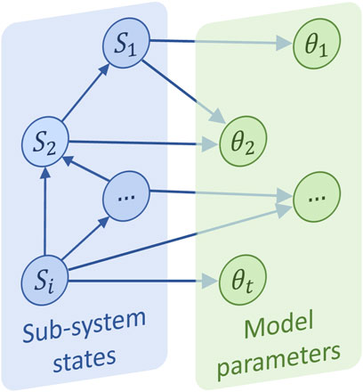
Figure 2. Bayesian Network for multi-model calibration.

Figure 3

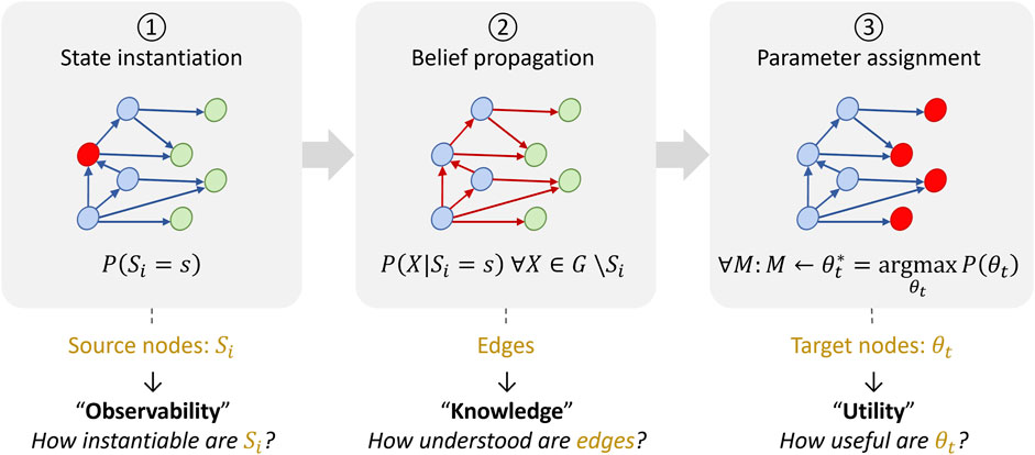
Figure 3. Calibration pipeline: Bayesian Network inference steps.

The proposed BN pruning method introduces three metrics evaluating the ability of specific graph components to serve the three steps of the calibration pipeline, namely, (1) observatbility $O(S_i)$; quantifies the instantiability of source nodes $S_i$, i.e., how easily can these nodes be observed, (2) knowledge $K(X_i\to X_j)$; quantifies the confidence in the ability of the arcs to represent causal relationships accurately, and (3) utility $U({\theta }_i)$; quantifies the expected usefulness of target nodes ${\theta }_i$ as some may be more important than others during operation. These metrics are assigned to components of the graph to be pruned as shown in Figure 4. For defining utility metrics, previous work proposed leveraging Failure Modes and Effect Analyses (FMEA) as these readily provide quantitative “severity” scores associated with risks in spacecraft operations (Gratius et al., 2024a). Using existing FMEA studies avoids conducting a dedicated knowledge elicitation campaign to evaluate this metric. This avoids elliciting expert knowledge specifically. The approach consists of summing over Risk Priority Numbers (RPNs) relevant to each parameter thereby defining a quantity representing how important a parameter is regarding the severity, occurrence, and detection of related risks: $U({\theta }_t)\triangleq \sum (RP{N}_{{\theta }_t})$. Metrics formulation for observability and knowledge however remains mostly undefined for multi-model calibration but some relevant methods will be discussed in a later section. Beyond the problem of defining these metrics appropriately, a more general challenge is to define an algorithmic framework integrating these metrics. This topic will be addressed in the next section before discussing individual metric definitions.

Figure 4

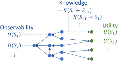
Figure 4. Metric assignment.

2.2 Proposed reduction method

We propose to prune the BN by solving an optimization problem intended to maximize the objective function in Equation 1. This equation first contains a performance part that sums over the metrics previously introduced and subtracts the KL divergence between the original and the pruned BN. The second part of the equation represents an expected computability score which is high if the computational cost of the BN is low. Finally, $\alpha$ and $\beta$ are weights, possibly multi-dimensional, to prioritize certain metrics over others. While these weights may prove to be difficult to estimate, there exist methods to facilitate their identification. For example, computing the Pareto front could help in identifying the solutions that are not dominated by others, thereby reducing the space of candidate values to explore (Van Veldhuizen and Lamont, 1998). All the terms in this equation will later be discussed in further detail, but we first introduce the associated pseudo-algorithm that we envision for solving the optimization problem.

$f\left(G\right)=\alpha {\displaystyle \underset{\mathcal{P}:\text{Performance}}{{\displaystyle \underbrace{\left({\displaystyle \sum _i}O\left(S_i\right)+{\displaystyle \sum _{S_i\to {\theta }_t}}K\left(X_j\to X_k\right)+{\displaystyle \sum _t}U\left({\theta }_t\right)-{KL}_G\right)}}}}+\beta \underset{\mathcal{C}:\text{Computability}}{\underbrace{\mathbb{E}\left[C^{+}\right]}}(1)$

The objective function previously defined is proposed to be maximized by following the steps described in Algorithm 1. First, a computability target $C_{\max }^{+}$ is defined, and the graph $G$ is pruned iteratively until the expected computability of the resulting BN reaches the target. At each iteration, the algorithm considers pruning candidate graph components and computes the resulting performance losses $L_i$. The candidates comprise all non-cut arcs and non-cut nodes to avoid the resulting graph being disconnected after pruning. We define a “non-cut” entity as a node or an arc, which can be pruned without separating the initial graph into multiple graph subsets. This term is used by opposition to the notion of separating set as defined in Chapter 4 of Douglas Brent (2001). The graph component eventually pruned is the one inducing the lowest loss. Note that graph components could be removed in batches but for simplicity, this algorithm considers removing unique components, i.e., removing a single arc or a single node at a time.

Algorithm 1

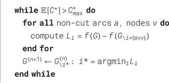
Algorithm 1.Bayesian Network pruning.

An example of the pruning process is illustrated in Figure 5 where nodes and arcs are iteratively considered for pruning. Note that once a node or arc is removed, the algorithm reiterates and goes through the remaining nodes and arcs. Each node keeps its identification label throughout the process as they embed an interpretable meaning, e.g., a node called “temperature” must keep that name for the end-user to interpret the graph as needed once the model is reduced and ready for use. The process stops when the computability target is achieved. We now discuss in more detail the different metrics that were introduced as part of this proposed optimization framework.

Figure 5

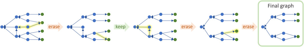
Figure 5. Example of iterative pruning.

2.3 Metric definition

The metrics integrated into the proposed pruning algorithm relate closely to existing practices. This section discusses how observability, knowledge, utility, KL divergence, and computability, can be defined for BN-based multi-model calibration by leveraging previous work.

2.3.1 Observability

In the control community, a system is said to be “observable” if its state can be entirely inferred from measurements (also called outputs). Such measurements can be obtained in aerospace systems using sensors, e.g., approximately 350,000 sensors are used in the International Space Station (ISS) (Wu and Vera, 2019). However, sensors may be subject to noise (Xu et al., 2021) and placement limitations (Guo et al., 2021) thereby limiting the quality of information that can be accessed. Alternatively, human operators can collect measurements. For example, in the ISS, maintenance time is estimated to be 2 hours per crew member per day and can include data collection tasks (Russell et al., 2006). This data collection method however also has limitations as human operators may not always be available. For example, in the future Gateway space habitat, crew members are expected to occupy the habitat only 30–60 days per year (Coderre et al., 2018).

As available measurements have limitations, it is reasonable to assume that some subsystems may be more easily observable than others. Previous work quantified observability probabilistically by counting the number of critical measurements without which a system becomes unobservable (Brown Do Coutto Filho et al., 2013). One contrast with such a method is that the BN architecture, on which our study is based, models the system as a set of connected nodes representing sub-systems. In this context, the concept of observability is only applied locally to individual nodes, i.e., we assume that external detection and diagnosis algorithms provide state estimates for each node. In this work, we envision that observability scores will be primarily derived from the detection score defined in FMEA studies. For example, the work in Eshima and Nabity (2020) defined a scale from 1 to 5 to quantify how detectable a given failure is.

2.3.2 Knowledge

We define knowledge as a metric representing how certain sub-systems experts are of the probabilities encoded by a specific arc. In BNs, an arc is formalized as a Conditional Probability Distribution (CPD) of the form: $P(\text{destination}|\text{origin})$. If this distribution is well known, i.e., there is significant prior information available to specify the distribution, the knowledge score is high and vice versa. We implemented this metric by assigning a number between 0 and 10 to each arc, where 0 indicates that the CPD of the arc is unknown and 10 indicates that the CPD is certain. This work assumes that the elicited experts are able to provide a reasonable estimate without relying on specific thresholds. Note that in addition to defining probabilities, arcs in BNs are also used to specify causal relationships between random variables. For example, an arc between two random variables, $A\to B$ can be read as “$A$ causes $B$” where $A$ could represent the rain, and $B$ represents whether the grass is wet or dry. Algorithms have been defined to learn the structure of the graphs from data (Spirtes and Glymour 1991; Spirtes et al., 2000), but these typically require a large amount of data, which may not be possible to collect in practice.

As causal relationships are often best understood by subject matter experts, several expert elicitation methods have been developed in that regard. For example, the Sheffield elicitation (SHELF) process is a step-by-step method to define CPDs. It consists of preparing evidence, conducting expert elicitation individually, conducting expert elicitation in a group, fitting the distribution to the collected answers, and finally, conducting a joint distribution elicitation (Rizzo and Blackburn, 2019). Other methods are more focused on the graph structure itself. For example, the authors in Xiao et al. (2018) elicit expert opinion by asking for a scalar value that is negative if the arc is believed to be inexistent and positive if it is believed to exist. The magnitude of the scalar value is used to represent the strength of the expert’s belief. In addition, expert accuracy is modeled using a standard deviation variable.

In this work, we assume that existing expert elicitation methods, such as the ones previously discussed, can be leveraged to define knowledge metrics for each arc quantifying the belief in both the resulting graph structure and the resulting probability distribution. While this implementation did not define specific thresholds for the knowledge scoring, such an approach could be considered in future work.

2.3.3 Utility

Utility is a metric that has been defined in previous work (Gratius et al., 2024a). It represents the expected usefulness of individual model parameters given previous information on operational conditions on similar aerospace systems. Such information can be derived from FMEA analysis such as the one proposed by the author in Eshima and Nabity (2020) to describe the risks associated with life support systems in space habitats.

2.3.4 KL divergence

As a BN represents joint distribution over its random variables, KL divergence can be computed between multiple BNs by considering their respective joint distribution. The joint distribution of a BN can be formulated as a factorization over its marginal and conditional distributions for each random variable $X_k$ (see Equation 2).

$p\left(x\right)=\prod _{k=1}^{K}p\left(X_k\mid \text{parent}\left(X_k\right)\right)(2)$

Explicitly specifying a closed-form solution for such joint distributions can be difficult in BNs, and so, these distributions are often estimated using sampling methods (Koller and Friedman, 2009). In this work, we sampled the BNs to be compared as described in Figure 6 to generate a data file for each network. We used Maximum a Posteriori estimation (MAP) to estimate probabilities for each node configuration. This consists of counting the number of configuration occurrences in each data file and normalizing by the number of data samples. Note that MAP is similar to combining Maximum Likelihood Estimation (MLE) with an informative prior. Specifically, we associated a low probability to all configurations before using the data to avoid assigning a probability of zero to configurations that did not appear in the data set because they were unlikely.

Figure 6

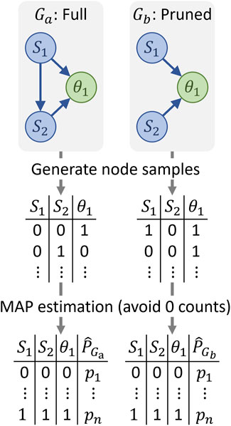
Figure 6. Sampling for KL divergence computation.

The computation of KL divergence is shown in Equation 3 where we use the following notation for clarity: $P(S_i=s_i)=P(s_i)$ and $P({\theta }_1=t_1)=P(t_1)$. Applying this formula to the example from Figure 6 results in Equation 4.

$KL\left(p\Vert q\right)={\displaystyle \sum _{i=1}^N}{p}_i{\log }_2\left(\frac{p_i}{q_i}\right)(3)$

$KL\left({\widehat{P}}_{G_a}\Vert {\widehat{P}}_{G_b}\right)={\displaystyle \sum _{\begin{array}{c}{s}_1,s_2,t_1\in \left\{\mathrm{0,1}\right\}\end{array}}^N}{\widehat{P}}_{G_a}\left(s_1,s_2,t_1\right){\log }_2\left(\frac{{\widehat{P}}_{G_a}\left(s_1,s_2,t_1\right)}{{\widehat{P}}_{G_b}\left(s_1,s_2,t_1\right)}\right)(4)$

After pruning, one of the BNs may have fewer nodes than the other, thereby leading to joint distributions over a distinct set of random variables. In this case, KL divergence would normally be either undefined or set to infinity as no configuration of random variables can be matched. Existing methods therefore tend to be limited to the computation of KL divergence across BN with the same nodes but with different arcs (Moral et al., 2021). Intuitively, this issue arises because the loss in nodes cannot be measured statistically as this is primarily a domain problem, i.e., the value of each node depends on the intended application downstream. Therefore, we propose to separate concerns by measuring the domain loss separately from the statistical loss. The domain loss is computed over the entire graphs by using utility, knowledge, and observability metrics. The statistical loss is measured only on the shared random variables by marginalizing out the nodes belonging to only one of the data files. Note that this marginalization approach is similar to the mechanisms employed in well-established belief propagation algorithms (Jensen and Nielsen, 2007). Additionally, sampling large BN and counting all node configurations may be computationally expensive for large networks. Methods have therefore been developed to reduce this cost by, for example, leveraging dynamic programming, i.e., using cache memory to reuse previous results rather than re-computing them.

2.3.5 Computability

We use the term computability to refer to the ease with which an algorithm can be computed, highlighting the efficiency and minimal computational resources required to achieve a solution. Two types of computational costs can be dissociated when considering computability issues in BN-based multi-model calibration problems, namely, direct and indirect costs. These costs can be associated with either the calibration itself or the simulation tasks downstream (see Figure 7). When designing a BN for multi-model calibration, the parameter nodes added to the graph are tied to an underlying choice in the type of simulation models that will be supported. In practice, if such models are intended to provide analysis support in anomaly response scenarios when operating an aerospace system, certain simulation needs may be more urgent than others. For example, using models to predict a small drift in cabin temperature over several months (Gratius et al., 2023), may be less time-critical than simulating the cabin depressurization rate following a meteorite (Rhee et al., 2023). This results in a need for balanced simulation capabilities where some models are better for accurate analysis while other models are prioritized for time-critical analyses. When pruning a BN for multi-model calibration one should therefore account for both (1) the direct cost of updating the BN to estimate parameters, and (2) the indirect expected costs associated with the underlying simulation models calibrated by the previously identified parameters.

Figure 7

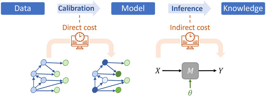
Figure 7. Direct and indirect computational costs: Model $M$, Input $X$, Output $Y$ (icons: Flaticon.com).

Indirect costs are more challenging to estimate than direct costs as their magnitudes and frequencies are tied to uncertain system operation queries. In particular, the cost of running a simulation model can vary greatly depending on the type of model and operational constraints. Such cost estimation could benefit from expanding existing simulation model libraries with computability information (FMI, 2023; Isasi et al., 2015). In this study, we choose to primarily focus on the direct cost for simplicity, i.e., we assume that parameters can be pruned without having a significant impact on the desired diversity of simulation capabilities downstream. While direct BN inference costs are also not easily identifiable, studies have shown that a BN with larger cliques typically induces high costs at inference time (Mengshoel, 2010). This is closely related to the growth of the junction tree and the number of BN parameters, i.e., the quantities defining marginal and conditional probability distribution in the BN. In the following, we will, therefore, set computability targets by specifying a reduction in the number of independent BN parameters, i.e., parameters that cannot be deduced from ensuring that probabilities sum to one. These BN parameters are meant to capture the updating behavior of the graph and are to be distinguished from the simulation model parameter represented by the green nodes in the network.

2.4 Validation method

2.4.1 Data-based validation

In the machine learning community, data-driven BNs are typically validated by splitting a dataset according to Figure 8. Training data is used to learn the parameters of the BN and test data is used after training to provide ground truths against which model predictions are compared. The difference between ground truths and predictions in the test data is used to evaluate an accuracy metric such as the Euclidian distance. In certain cases, the data is split three-fold to define a validation dataset which is typically used for hyperparameter selection. Figure 8b illustrates the cross-validation approach which is another popular method consisting of alternating between different validation and training data splits to avoid overfitting.

Figure 8

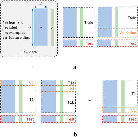
Figure 8. Validation principles: (a) General validation. (b) Cross-validation.

One of the limitations of the previously discussed validation methods is their reliance on available datasets. Data tend to be difficult to obtain in hybrid BN, i.e., BN derived from both data and domain knowledge. This is the case for multi-model calibration as collecting data would require retrieving many instances of model calibration given the states of an aerospace system. Historical records of this type exist, for example, from the operation of the Space shuttle (Watts-Perotti and Woods, 2007), but they remain sparse and difficult to collect.

2.4.2 Hybrid validation

In this work, we deployed three hybrid validation approaches because of their demonstrated applicability to BN which do not rely solely on data as described in Pitchforth and Mengersen (2013). The two first approaches are relatively brief and discussed hereafter, and the third one will be covered in the next section.

First, nomological validity consists of ensuring that the designed BN belongs to a literature-established domain. We identified a significant corpus of literature confirming this validity criterion. This include BN representing system states (Hwang et al., 2023; Gratius et al., 2023; O’Neill et al., 2019; Mindock and Klaus, 2012), representing model parameters (Li et al., 2017; Ye et al., 2020; Sankararaman and Mahadevan, 2015), and embedding multiple simulation models (Kaghazchi et al., 2021; Tao et al., 2021). Second, convergent validity verifies that the proposed BN is similar to nomologically proximal BNs. One relevant example is the work presented in kapteyn et al. (2021) for digital twin-based operations of aerospace systems. The inference steps employed are closely related to the ones employed in our work as they consist of (1) collecting data, (2) inferring the system state, and (3) conducting simulations to analyze the quantity of interest. The third, and most extensive, validation approach for hybrid BNs is predictive validity. This approach is very similar to the ones traditionally used for data-driven BNs as it quantitatively compares the output and behavior of a proposed BN with an alternative BN. We therefore aim at introducing and comparing two BNs: (1) a BN pruned with well-established statistical methods, and (2) a BN pruned using a combination of statistical and domain-driven approaches. Note that our objective is to validate the pruning procedure rather than the BN itself. However, comparing the behaviors of BNs resulting from alternative pruning procedures is useful to provide insights for the evaluation of our method against existing approaches.

2.4.3 Predictive validity

The method we deploy for predictive validity starts by defining the initial graph to be pruned which we refer to as $G_0$. Because all models are approximations, we also define a true BN, which is normally unknown at the time of pruning, but will be useful later on. This true graph is referred to as $G_{\mathit{true}}$. The objective is therefore to prune a BN $G_0$, which is an approximation of a true BN $G_{\mathit{true}}$. After setting a computational target, $G_0$ is pruned using both the baseline and the proposed methods to generate the BNs $G_b$ and $G_p$ respectively as shown in Figure 9.

Figure 9

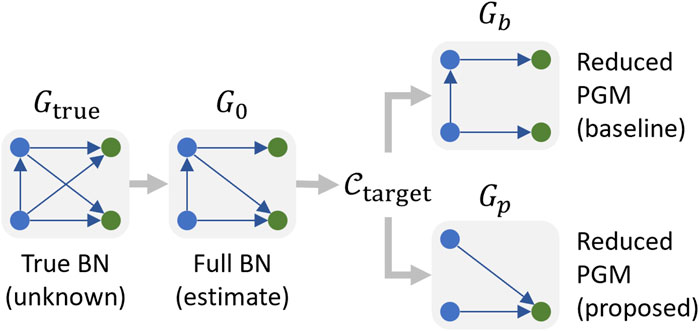
Figure 9. Validation pipeline.

The objective of the validation consists of ensuring that if the $O,K,U$ metrics are informative, i.e., at least better than random guesses, the BN resulting from the proposed method should demonstrate better predictive performance in its estimate of model parameters. The following steps will be conducted.

1. Define the ground truth BN $G_{\mathit{true}}$

2. Define $G_0$ as a copy of $G_{\mathit{true}}$, and assign metric scores as follows:

• Knowledge $K$: Introduce mistakes in $G_0$, i.e., BN properties that are different from $G_{\mathit{true}}$, and compensate for them by defining low $K$ scores on the impacted arrows. For example, if a conditional distribution becomes noisy as shown in Figure 10, the $K$ score associated with that arrow should be low in most cases.

• Observability $O$: Assign observation scores to system nodes to serve as probabilistic filters. For example, if the node “valve” has a score of 0.6, then in 40% of the trials where this node is instantiated, the state will be incorrect, e.g., “nominal” instead of “degraded”.

• Utility $U$: Assign utility scores to parameter nodes to reflect how often we expect each node to be the object of a query. For example, if a parameter node has a parent representing a system with a high probability of failure, its utility is likely to be high.

3. The baseline and proposed pruning methods are then implemented to obtain $G_b$ and $G_p$

4. These BNs are used to predict parameters on sample sets comprising both system evidence and parameter queries, e.g., “What is the most likely value of ${\theta }_i$ given that the subsystem $S_j$ is degraded?“. These queries are defined by (1) sampling that state nodes in $G_{\mathit{true}}$, (2) applying the probabilistic filtering specified by $O$, (3) defining the parameter of interest as the parameter node(s) most closely connected to the degraded system node(s).

5. Finally, for each query, the predicted parameters for both pruned BNs are classified as correct or incorrect by comparing these with the prediction of $G_{\mathit{true}}$.

Figure 10

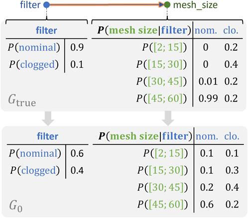
Figure 10. Example of noisy distribution.

Note that the metrics previously defined are only required to be partially correct, i.e., better than average in their ability to inform on the quality of graph components in $G_0$. The BN used for $G_0$ is derived from the work presented in Gratius et al. (2024a) which is shown in Figure 11. This BN represents a space habitat called Gateway which can be crewed and is composed of modules, namely, the Power and Propulsion Element (PPE), the International Habitat (I-HAB), and the Habitation and Logistics Outpost (HALO). The graph further expands on the Environmental Control and Life Support System (ECLSS) which comprises a Carbon Dioxide Removal System (CDRS), an Air Circulation and Ventilation (ACV) unit, an Oxygen Generation Assembly (OGA), a Fire Detection and Suppression (FDS) system, a Water Processing Assembly (WPA), and a Temperature and Humidity Control System (THCS). Green nodes on the right-hand side are parameters associated with different models as described in Gratius et al. (2024a). Figure 11 highlights the graph components where informative metrics $(O,K,U)$ have been assigned. The structure for $G_0$ and $G_{true}$ were kept the same but some of the underlying probabilities were modified as described previously. The graph structure was maintained for simplicity but this will not bias the evaluation towards one of the pruning methods as both methods start from the same graph $G_0$.

Figure 11

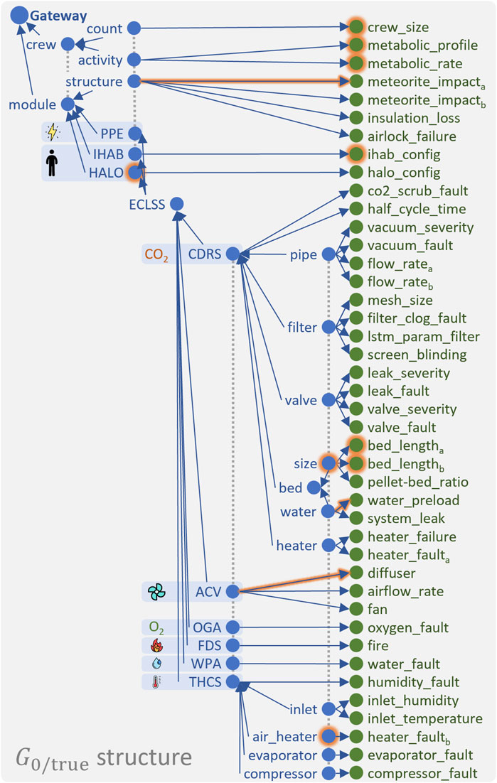
Figure 11. BN to prune: informative metrics $(O,K,U)$ were assigned to nodes and arrows with glowing contours (icons: Flaticon.com).

3 Results

The results presented in this section were generated using BayesFusion software, namely, the GeNIe modeler (BayesFusion, 2023a) and its SMILE engine (BayesFusion, 2023b) that we accessed through its Python Application Programming Interface (API) called PySMILE. The software code designed for this case study is publicly available on GitHub (Gratius et al., 2024b).

3.1 Verification

This first step consists of verifying that the pruning algorithms for the baseline and the proposed methods are executing their tasks as expected, especially concerning the performance objective function. Figure 12 shows the pruning of the same graph $G_0$ for three computational targets, namely, reductions of 5%, 10%, and 20%. These percentages correspond to reductions in the number of independent BN parameters, e.g., $\{Target=10\%\wedge |{\theta }_{\mathit{old}}|=50\}\Rightarrow |{\theta }_{\mathit{new}}|=45$. Each point $b_n$ and $p_n$ in the figures represents a newly pruned graph and the pruning stops once the computational target has been achieved. In each case, the performance score achieved by the latest graph in the proposed method has a better performance score than the baseline. This is expected because the baseline considers only KL divergence while the proposed method optimizes over the performance metric itself which compounds KL divergence with the $O,K,U$ metrics and the expected computability $\mathbb{E}[C^{+}]$, which we simply defined as the number of independent parameters.

Figure 12

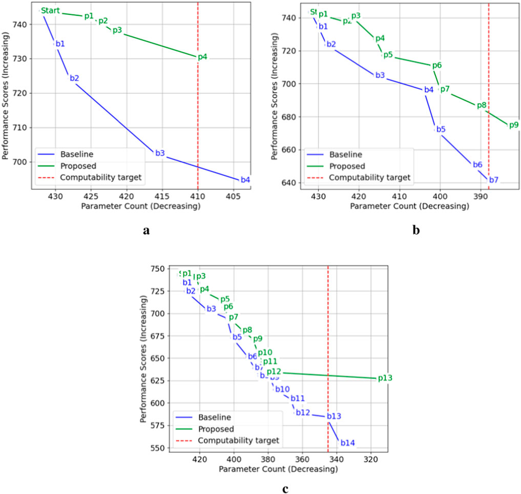
Figure 12. Performance VS Parameters. (a): Pruning with 5% reduction (b) Pruning with 10% reduction (c) Pruning with 20% reduction.

3.2 Validation

Similarly, for validation, we pruned $G_0$ with both the baseline and the proposed method for three distinct computational targets. As discussed, queries were then generated by (1) sampling the system nodes from $G_{\mathit{true}}$, (2) applying the observability filtering, and (3) defining the parameter(s) to be retrieved. Note that for this last step, we assume that the correct parameter of interest can be specified correctly in the query even if an incorrect observation has been made. This is to simplify result interpretation as the BN is primarily used here for parameter estimation rather than diagnosis. The results are shown in Figure 13 which shows that the proposed method consistently outperforms the baseline even as the target reduction becomes more stringent.

Figure 13

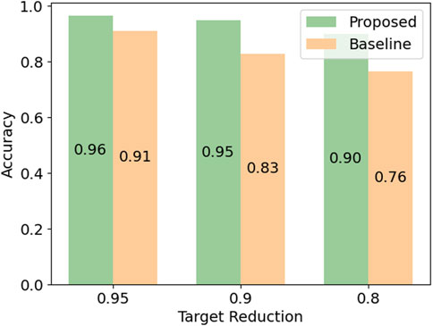
Figure 13. Accuracy of the proposed and the baseline method for different computational reduction targets.

4 Discussion

We now discuss some of the lessons learned we discovered in this study by reviewing implementation details and limitations that could be considered for future work.

4.1 Observations

We made three implementation adjustments to ensure computational tractability and fairness in comparing the methods. First, existing KL divergence-based methods for pruning BNs are primarily focused on removing arcs (Kjaerulff, 1994). This however bounds the reduction target as the number of non-cut arcs is limited. For a fair comparison, we extended this method to also prune nodes once all non-cut arcs have been removed. Nodes were selected using the same KL divergence criteria as for arcs. Second, as the network considered in our work is relatively large, we chose, for the proposed method, to only measure the KL divergence between the parameter nodes as these are the nodes that we ultimately are interested in. We expect this approximation to be reasonable and more informative given the intended application. However, in the baseline method, we kept measuring KL divergence for all the nodes to mirror existing practices as these do not prioritize which node to select based on their expected future use. Thirdly, during pruning, the algorithm may choose to remove a parameter node. This may lead to a conflict when defining the queries as these may refer to parameter nodes that are not in the reduced graphs anymore. Instances where such queries occurred were systematically classified as incorrect.

4.2 Limitations

Defining weights for quantities in the objective function can be challenging as there is no obvious calibration procedure for such hyperparameters. We found that (1) the scale of the KL divergence should be similar to the scale used by the $O,K,U$ metrics, thereby avoiding imbalanced representations, and (2) no weight adjustments were required for the $O,K,U$ metrics to perform appropriately. Further studies should investigate whether adjusting the weight $\alpha ,\beta$ beyond ensuring a similar scale for all metrics could improve the reduction process.

An additional issue is that computing KL divergence between BNs using samples is very computationally demanding. The graph in this study was reduced within five to 15 minutes depending on the reduction target (using an 11th Gen Intel Core i7-1185G7 @ 3.00 GHz with 32 GB RAM on Windows 11). A larger graph may not be tractable. We found that an efficient way to save costs was to generate a unique and relatively large sample set from $G_{\mathit{true}}$ at the beginning of the algorithm, and smaller sample sets for candidate BNs. This is because generating many samples for all the candidates tends to significantly increase computational demand. The tradeoff in this approach consists of choosing between a large number of samples, resulting in a more accurate estimation of the KL divergence, and a smaller sample set, which reduces the computational cost of the reduction algorithm.

Moreover, the number of entities being pruned at a time may have an influence on the resulting BN, e.g., pruning several nodes at a time may lead to better results than pruning a single node at a time. Future work could attempt deploying iterative strategies where pruning is done according to different batch sizes to avoid local maxima when optimizing according to the objective function. Pruning multiple nodes and arcs at a time will increase the computational cost of the reduction because the number of candidate graph subsets to be removed will be larger. However, this may also help in avoiding local maxima in the objective function, which may be induced when pruning single entities. The tradeoff between the computational cost of the reduction and the gain in inference capabilities for the resulting BN could be studied in future work.

Finally, further studies may be conducted on expanding the scope of the objective function. The main goal is to improve the computational tractability of performing inference on the resulting graph after pruning. The optimization approach presented in this paper consists of pruning graph entities such that the loss in the objective function is minimal, i.e., the loss in parameter selection accuracy is minimized. Ultimately, the final purpose of the reduced BN is to infer the parameters of other downstream models, which will be used for simulations. A more general objective function could be defined to measure the loss of accuracy for the downstream simulation outputs. Specifically, even if a selected parameter is the most appropriate one out of multiple candidates, the associated model is still an approximation of reality and will, therefore, lead to inaccuracies. Future work could consider incorporating post-simulation analysis to reinforce uncertainty-aware decision-making.

5 Conclusion

To conclude, we introduced a method to prune BNs for computationally tractable multi-model calibration. While existing BN pruning methods rely primarily on statistics, these can benefit from incorporating domain knowledge when selecting graph components to be pruned. This work is deployed on a space habitat example and the parameter prediction accuracy of the proposed method outperforms existing practices relying solely on statistics. Future work could benefit from defining how weights should be assigned to the decision metrics and how different batch sizes should be considered when pruning a BN.

Data availability statement

The original contributions presented in the study are included in the article/supplementary material, further inquiries can be directed to the corresponding author.

Author contributions

NG: Conceptualization, Data curation, Formal Analysis, Funding acquisition, Investigation, Methodology, Project administration, Resources, Software, Supervision, Validation, Visualization, Writing – original draft, Writing – review and editing. MB: Conceptualization, Data curation, Formal Analysis, Funding acquisition, Investigation, Methodology, Project administration, Resources, Software, Supervision, Validation, Visualization, Writing – original draft, Writing – review and editing. BA: Conceptualization, Data curation, Formal Analysis, Funding acquisition, Investigation, Methodology, Project administration, Resources, Software, Supervision, Validation, Visualization, Writing – original draft, Writing – review and editing.

Funding

The author(s) declare that financial support was received for the research and/or publication of this article. This work was supported by the National Aeronautics and Space Administration (NASA) as part of the Space Technology Research Institute (STRI) Habitats Optimized for Missions of Exploration (HOME) “SmartHab” project (grant number 80NSSC19K1052) and by Carnegie Mellon University (CMU) through the Dean’s Fellowship from the College of Engineering.

Conflict of interest

MB holds concurrent appointments as a Professor of Civil and Environmental Engineering at Carnegie Mellon University and as an Amazon Scholar. This paper describes work at Carnegie Mellon University and is not associated with Amazon.

The remaining authors declare that the research was conducted in the absence of any commercial or financial relationships that could be construed as a potential conflict of interest.

Generative AI statement

The author(s) declare that no Generative AI was used in the creation of this manuscript.

Publisher’s note

All claims expressed in this article are solely those of the authors and do not necessarily represent those of their affiliated organizations, or those of the publisher, the editors and the reviewers. Any product that may be evaluated in this article, or claim that may be made by its manufacturer, is not guaranteed or endorsed by the publisher.

Author disclaimer

Any opinions, findings, conclusions, or recommendations expressed in this material are those of the authors and do not necessarily reflect the views of NASA or CMU.

References

AIAA and AIA (2020). Digital twin institute position paper. AIAA. Available online at: https://www.aia-aerospace.org/publications/digital-twin-definition-value-an-aiaa-and-aia-position-paper/

Google Scholar

Alizadeh, R., Allen, J. K., and Mistree, F. (2020). Managing computational complexity using surrogate models: a critical review. Res. Eng. Des. 31, 275–298. doi:10.1007/s00163-020-00336-7

CrossRef Full Text | Google Scholar

BayesFusion (2023a). GeNIe modeler – BayesFusion

Google Scholar

BayesFusion (2023b). SMILE engine – BayesFusion

Google Scholar

Blochwitz, T., Otter, M., Akesson, J., Arnold, M., Clauß, C., Elmqvist, H., et al. (2012). “Functional mockup Interface 2.0: the standard for tool independent exchange of simulation models,” in Proceedings (münchen). doi:10.3384/ecp12076173

CrossRef Full Text | Google Scholar

Brown Do Coutto Filho, M., de Souza, J. C. S., and Villavicencio Tafur, J. E. (2013). Quantifying observability in state estimation. IEEE Trans. Power Syst. 28, 2897–2906. doi:10.1109/TPWRS.2013.2241459

CrossRef Full Text | Google Scholar

Chu, R. R. (2002). “ISS ECLS system analysis software tools - an overview and assessment,” in International conference on environmental systems (SAE international), 8. doi:10.4271/2002-01-2343

CrossRef Full Text | Google Scholar

Coderre, K. M., Edwards, C., Cichan, T., Richey, D., Shupe, N., Sabolish, D., et al. (2018). “Concept of operations for the Gateway,” in 2018 SpaceOps conference (American Institute of Aeronautics and Astronautics), SpaceOps conferences, 1–14. doi:10.2514/6.2018-2464

CrossRef Full Text | Google Scholar

Dempsey, R. (2018). “Day in the life: when a major anomaly occur,” in The international space station: operating an Outpost in the new frontier (Government Printing Office), Houston, Texas: NASA. 354–377. Available online at: http://www.nasa.gov/connect/ebooks/the-international-space-station-operating-an-outpost

Google Scholar

Douglas Brent, W. (2001). Introduction to graph theory, 2. Upper Saddle River: Prentice-Hall.

Google Scholar

Eshima, S., and Nabity, J. (2020). “Failure mode and effects analysis for environmental control and life support system self-awareness,” in 2020 international Conference on environmental systems (lisbon, Portugal: 2020 international conference on environmental systems), 13.

Google Scholar

FMI (2023). Functional mock-up Interface specification. Standard 3.0.1, FMI

Google Scholar

Gratius, N., Berges, M., and Akinci, B. (2024a). Designing PGM-based multi-model calibration: a deep space habitat study. preprint.

Google Scholar

Gratius, N., Bergés, M., and Akinci, B. (2024b). Available online at: https://github.com/ngratius/bayesian-network-pruning.

Google Scholar

Gratius, N., Bergés, M., and Akinci, B. (2024c). “Integrated calibration of simulation models for autonomous space habitat operations,” in 2024 IEEE aerospace conference big sky, 18. MT, USA: IEEE. doi:10.1109/AERO58975.2024.10520995

CrossRef Full Text | Google Scholar

Gratius, N., Hou, Y., Bergés, M., and Akinci, B. (2023). Lessons learned on the implementation of probabilistic graphical model-based digital twins: a space habitat study. J. Space Saf. Eng. 10, 172–181. doi:10.1016/j.jsse.2023.04.001

CrossRef Full Text | Google Scholar

Gratius, N., Wang, Z., Hwang, M. Y., Hou, Y., Rollock, A., George, C., et al. (2024d). Digital twin technologies for autonomous environmental control and life support systems. J. Aerosp. Inf. Syst. 21, 332–347. doi:10.2514/1.I011320

CrossRef Full Text | Google Scholar

Guo, Y., Xu, Z., and Saleh, J. H. (2021). “Active sensing for space habitat environmental monitoring and anomaly detection,” in 2021 IEEE aerospace conference (50100) big sky (MT, USA: IEEE), 1–12. doi:10.1109/AERO50100

CrossRef Full Text | Google Scholar

Hwang, M. Y., Akinci, B., and Bergés, M. (2023). Updating subsystem-level fault-symptom relationships for Temperature and Humidity Control Systems with redundant functions. J. Space Saf. Eng. 11. doi:10.1016/j.jsse.2023.10.010

CrossRef Full Text | Google Scholar

Isasi, Y., Noguerón, R., and Wijnands, Q. (2015). “Simulation Model Reference Library: a new tool to promote simulation models reusability,” in Workshop on simulation for European space programmes (SESP) 2015, 8. Noordwijk-Nederlands: SESP.

Google Scholar

Jensen, F. V., and Nielsen, T. D. (2007). Bayesian networks and decision graphs. 2 edn. Springer.

Google Scholar

Kaghazchi, A., Hashemy Shahdany, S. M., and Roozbahani, A. (2021). Simulation and evaluation of agricultural water distribution and delivery systems with a Hybrid Bayesian network model. Agric. Water Manag. 245, 106578. doi:10.1016/j.agwat.2020.106578

CrossRef Full Text | Google Scholar

kapteyn, M. G., Pretorius, J. V. R., and Willcox, K. E. (2021). A probabilistic graphical model foundation for enabling predictive digital twins at scale. Nat. Comput. Sci. 1, 337–347. doi:10.1038/s43588-021-00069-0

PubMed Abstract | CrossRef Full Text | Google Scholar

Kjaerulff, U. (1994). “Reduction of computational complexity in bayesian networks through removal of weak dependences,” in Uncertainty in artificial intelligence. Editors R. L. de Mantaras, and D. Poole (San Francisco (CA): Morgan Kaufmann), 374–382.

Google Scholar

Koller, D., and Friedman, N. (2009). Probabilistic graphical models: principles and techniques. MIT Press). Google-Books-ID: 7dzpHCHzNQ4C.

Google Scholar

Kullback, S., and Leibler, R. A. (1951). On information and sufficiency. Ann. Math. Statistics 22, 79–86. doi:10.1214/aoms/1177729694

CrossRef Full Text | Google Scholar

Lara, J. D., Henriquez-Auba, R., Ramasubramanian, D., Dhople, S., Callaway, D. S., and Sanders, S. (2023). Revisiting power systems time-domain simulation methods and models. IEEE Trans. Power Syst. 39, 2421–2437. ArXiv:2301.10043 [cs, eess]. doi:10.1109/TPWRS.2023.3303291

CrossRef Full Text | Google Scholar

Li, C., and Mahadevan, S. (2018). Efficient approximate inference in Bayesian networks with continuous variables. Reliab. Eng. and Syst. Saf. 169, 269–280. doi:10.1016/j.ress.2017.08.017

CrossRef Full Text | Google Scholar

Li, C., Mahadevan, S., Ling, Y., Choze, S., and Wang, L. (2017). Dynamic bayesian network for aircraft wing health monitoring digital twin. AIAA J. 55, 930–941. doi:10.2514/1.J055201

CrossRef Full Text | Google Scholar

Margolis, B. W. l., and Lyons, K. R. (2022). SimuPy flight vehicle toolkit. J. Open Source Softw. 7, 4299. doi:10.21105/joss.04299

CrossRef Full Text | Google Scholar

Mengshoel, O. J. (2010). Understanding the scalability of Bayesian network inference using clique tree growth curves. Artif. Intell. 174, 984–1006. doi:10.1016/j.artint.2010.05.007

CrossRef Full Text | Google Scholar

Mindock, J., and Klaus, D. (2012). “Development and application of spaceflight performance shaping factors for human reliability analysis,” in 41st international conference on environmental systems (Portland, Oregon, USA: American Institute of Aeronautics and Astronautics), 15. doi:10.2514/6.2011-5158

CrossRef Full Text | Google Scholar

Montero Jimenez, J. J., Schwartz, S., Vingerhoeds, R., Grabot, B., and Salaün, M. (2020). Towards multi-model approaches to predictive maintenance: a systematic literature survey on diagnostics and prognostics. J. Manuf. Syst. 56, 539–557. doi:10.1016/j.jmsy.2020.07.008

CrossRef Full Text | Google Scholar

Moral, S., Cano, A., and Gómez-Olmedo, M. (2021). Computation of kullback–leibler divergence in bayesian networks. Entropy 23, 1122. Number: 9 Publisher: Multidisciplinary Digital Publishing Institute. doi:10.3390/e23091122

PubMed Abstract | CrossRef Full Text | Google Scholar

O’Neill, J., Bowers, J., Corallo, R., Torres, M., and Stapleton, T. (2019). “Environmental control and life support module architecture for deployment across deep space platforms,” in Publisher: 49th international Conference on environmental systems (boston, Massachusetts: ICES), 10. Publisher: 49th international conference on environmental systems.

Google Scholar

Pitchforth, J., and Mengersen, K. (2013). A proposed validation framework for expert elicited Bayesian Networks. Expert Syst. Appl. 40, 162–167. doi:10.1016/j.eswa.2012.07.026

CrossRef Full Text | Google Scholar

Rhee, S., Noble, Z., Park, J., Lial, A., Collazo, C. L., and Davide, Z. (2023). “Development of a damageable ECLSS and interior-environment virtual testbed model to simulate future resilient deep space habitats,” in 2023 international conference on environmental systems, 15. Calgary, Canada: ICES.

Google Scholar

Rizzo, D. B., and Blackburn, M. R. (2019). Harnessing expert knowledge: defining bayesian network model priors from expert knowledge only—prior elicitation for the vibration qualification problem. IEEE Syst. J. 13, 1895–1905. doi:10.1109/JSYST.2019.2892942

CrossRef Full Text | Google Scholar

Russell, J. F., Klaus, D. M., and Mosher, T. J. (2006). Applying analysis of international space station crew-time utilization to mission design. J. Spacecr. Rockets 43, 130–136. doi:10.2514/1.16135

CrossRef Full Text | Google Scholar

Sankararaman, S., and Mahadevan, S. (2015). Integration of model verification, validation, and calibration for uncertainty quantification in engineering systems. Reliab. Eng. and Syst. Saf. 138, 194–209. doi:10.1016/j.ress.2015.01.023

CrossRef Full Text | Google Scholar

Spirtes, P., and Glymour, C. (1991). An algorithm for fast recovery of sparse causal graphs. Soc. Sci. Comput. Rev. 9, 62–72. doi:10.1177/089443939100900106

CrossRef Full Text | Google Scholar

Spirtes, P., Glymour, C. N., and Scheines, R. (2000). Causation, prediction, and search. Cambridge, MA, USA: MIT Press.

Google Scholar

Tao, S., van Beek, A., Apley, D. W., and Chen, W. (2021). Multi-model bayesian optimization for simulation-based design. J. Mech. Des. 143. doi:10.1115/1.4050738

CrossRef Full Text | Google Scholar

Van Veldhuizen, D., and Lamont, G. (1998). “Evolutionary computation and convergence to a pareto front,” in Late breaking papers at the genetic programming 1998 conference, 221–228.

Google Scholar

Watts-Perotti, J., and Woods, D. D. (2007). How anomaly response is distributed across functionally distinct teams in space shuttle mission control. J. Cognitive Eng. Decis. Mak. 1, 405–433. doi:10.1518/155534307X264889

CrossRef Full Text | Google Scholar

Wu, S.-C., and Vera, A. H. (2019). Supporting crew Autonomy in deep space exploration: preliminary onboard capability Requirements and proposed research questions. Technical Report of the autonomous crew operations technical interchange meeting. Tech. Rep. NASA/TM—2019–220345,.

Google Scholar

Xiao, C., Jin, Y., Liu, J., Zeng, B., and Huang, S. (2018). Optimal expert knowledge elicitation for bayesian network structure identification. IEEE Trans. Automation Sci. Eng. 15, 1163–1177. doi:10.1109/tase.2017.2747130

CrossRef Full Text | Google Scholar

Xu, Z., Guo, Y., and Saleh, J. H. (2021). Deep learning for the next generation (highly sensitive and reliable) ECLSS fire monitoring and detection system. IEEE Aerosp. Conf. 50100, 1–11. doi:10.1109/AERO50100.2021.9438141

CrossRef Full Text | Google Scholar

Ye, Y., Yang, Q., Yang, F., Huo, Y., and Meng, S. (2020). Digital twin for the structural health management of reusable spacecraft: a case study. Eng. Fract. Mech. 234, 107076. doi:10.1016/j.engfracmech.2020.107076

CrossRef Full Text | Google Scholar

Nomenclature

ACV Air Circulation and Ventilation

API Application Programming Interface

BNs Bayesian Networks

CDRS Carbon Dioxide Removal System

CPD Conditional Probability Distribution

ECLSS Environmental Control and Life Support System

FDS Fire Detection and Suppression

FMEA Failure Modes and Effect Analyses

HALO Habitation and Logistics Outpost

I-HAB International Habitat

ISS International Space Station

KL Kullback Leibler

MAP Maximum a Posteriori estimation

MCC Mission Control Center

MCMC Markov Chain Monte Carlo

MLE Maximum Likelihood Estimation

OGA Oxygen Generation Assembly

PGMs Probabilistic Graphical Models

PPE Power and Propulsion Element

RPNs Risk Priority Numbers

SHELF Sheffield elicitation

THCS Temperature and Humidity Control System

WPA Water Processing Assembly