DL-based organism-level microbial identification via VOCs fingerprints through gas chromatography – ion mobility spectrometry

Introduction: Organism-level microbial identification is a well-established topic in literature. Due to biosafety concerns, specifically identifying pathogenic bacteria is of critical importance. This study positions Deep Learning (DL) - based chemometric analysis as a promising strategy for organism-level microbial identification, with potential translational value for rapid diagnostics. Various chemometric methods have been applied to analyze pure and mixed cultures of microorganisms and generate data via Volatile Organic Compounds (VOCs) fingerprints for classification. Although Gas Chromatography - Ion Mobility Spectrometry (GC-IMS) is a promising chemometric technique in this field, limited research has explored its potential for organism-level microbial identification.

Materials and methods: In this study, GC-IMS prototypes were employed to generate two-dimensional spectral data, which were then used to train supervised classification models. Utilizing a publicly available dataset of four microorganisms, we conduct a series of experiments to perform multi-class classification of pure and mixed cultures. Additionally, we introduce innovative experiments for distinguishing bacteria from fungi and Gram-positive from Gram-negative bacteria. We further investigate the presence and pureness of two pathogenic bacteria, Escherichia coli and Pseudomonas fluorescens, within the cultures. To achieve this, we apply eight Machine Learning and DL baseline methods, while following a five-fold cross-validation evaluation protocol and presenting a wide set of evaluation metrics to ensure result reproducibility and models’ generalization. A further evaluation of DL models is also conducted to report the training times and the number of parameters of the proposed DL methods.

Results: Our key findings highlight a Fully Connected Neural Network (FCNN) with four hidden layers as the most efficient model, consistently achieving the best performance across all tasks in comparison to the other tested models of this study. Additionally, the FCNN model provides fast training and maintains a relatively small number of parameters compared to other DL approaches.

Discussion: While the dataset’s limited size and class imbalance present challenges such as potential overfitting and optimistic bias, the results achieved so far are encouraging and demonstrate the model’s strong potential. Future work should aim to expand the dataset across multiple sites and instruments and include clinical validation on real-world samples to further enhance generalizability and ensure translational impact.

1 Introduction

Bacteria are microscopic, single-celled microorganisms lacking a nuclear membrane (Baron, 1996). They are metabolically active and divide through binary fission. Despite their seemingly simple structure, bacteria are highly advanced and adaptable organisms capable of causing a wide range of diseases. Pathogenic bacteria, in particular, are associated with specific illnesses such as the plague (Feng et al., 2021). The diagnosis of bacterial infections and the efficient treatment of infectious diseases are critical for human health (Yang et al., 2024). Additionally, to minimize the risk of contamination and toxicity, bacterial detection plays a vital role in the quality control of food products such as yogurt, cheese, and beer, as well as in the monitoring of bacteria in crops and silage (Sauer and Kliem, 2010). A wide range of laboratory techniques can be employed for the taxonomic classification and identification of bacteria (Chauhan et al., 2020; Zukowska, 2021). Gram-positive and Gram-negative bacteria possess different cell wall structures, influencing their susceptibility to antibiotics. Consequently, determining the Gram type of bacteria is essential for selecting the most effective antibiotic treatment (Rezaei et al., 2024). Furthermore, different pathogens necessitate distinct management strategies; for instance, bacterial infections may require immediate antibiotic intervention, whereas fungal infections might need prolonged antifungal therapy (Giuliano et al., 2019).

Certain strains of Escherichia coli, such as E. coli O157:H7, are known to cause severe foodborne illnesses, including diarrhea, urinary tract infections, and kidney failure (Yang et al., 2017), while E. coli O157:47 is described as a category B biological warfare agent by the Centers for Disease Control and Prevention (CDC; Atlanta, GA, USA) (Pohanka, 2019), marking its accurate detection as an important concept in the literature. Although generally considered of low clinical significance, Pseudomonas fluorescens can either cause opportunistic infections, particularly in immunocompromised patients, including those with advanced cancer (Ishii et al., 2024) or have a significant impact in agriculture as a major food contaminant (Nunes et al., 2024). Most of these infections have been bloodstream infections, with few reports of pneumonia. Another bacterium, Levilactobacillus brevis, is commonly utilized in the fermentation of foods such as sauerkraut, kimchi, and pickles (Jeon et al., 2024). Detecting this bacterium ensures the quality and consistency of these fermented products. Regarding fungi, Saccharomyces cerevisiae is employed as a probiotic to prevent and treat various gastrointestinal diseases, such as antibiotic-associated diarrhea (Li et al., 2024). Detecting this yeast in probiotic products ensures they contain the intended beneficial strains. Concretely, the early detection and classification of these bacteria are essential for preventing outbreaks and mitigating biological threats.

Bacteria have been identified using various analytical methods, including molecular biology techniques such as polymerase chain reaction (PCR) for microorganisms, and immunological techniques such as enzyme-linked immunosorbent assays (ELISAs) for both protein toxins and microorganisms (Aboutalebian et al., 2021; Kim and Kim, 2021). While these methods are valuable for rapid screening of samples, they possess analytical limitations, including a lack of specificity, which can result in false positives due to cross-reactions with similar molecules. Furthermore, these methods are not suitable for the classification of unknown microbial samples (Duriez et al., 2016).

Conversely, mass spectrometry (MS) facilitates the unambiguous detection of microorganisms and protein toxins (Duriez et al., 2016). MS integrates speed, sensitivity, and specificity within a single technique, making it suitable for both targeted and untargeted detection of microorganisms, even in complex samples such as air, water, culture media, bodily fluids, and food (Tait et al., 2014; Altaee et al., 2017; Hameed et al., 2018). MS-based methodologies for identifying microorganisms through Volatile Organic Compounds (VOCs) fingerprints and toxins have continuously advanced with the development of soft ionization techniques, including matrix-assisted laser desorption/ionization (MALDI) and electrospray ionization (ESI), as well as high-resolution and high-mass-accuracy instruments (Dybwad, 2013; Su et al., 2022). These advancements have significantly enhanced the capability to accurately identify microorganisms and toxins, thereby ensuring biosafety across various contexts. Matrix-assisted laser desorption/ionization time of-flight mass spectrometry (MALDI-TOF MS) was one of the pioneering approaches for environmental applications. It is now recognized as a rapid, efficient, and reproducible method for species-specific identification of pathogenic microorganisms through the direct analysis of intact bacterial cells (Clark et al., 2013; Dingle and Butler-Wu, 2013). Specifically, MALDI-TOF MS, combined with advanced chemometric methods such as unsupervised clustering and classification using Artificial Neural Networks (ANN), has been employed to achieve rapid and reliable identification of bacteria from the genus Yersinia. MS-based methods have also been effectively applied to the identification and specific detection of biological agents by analyzing intact proteins and/or tryptic digests from bacterial cells (Lasch et al., 2010). However, under these conditions, MALDI-TOF analysis may lack sensitivity and is typically performed following a preliminary bacterial cultivation step, which serves both as a separation and enrichment tool. Additionally, various studies have investigated the capability of Orbitrap-MS prototypes to identify specific pathogenic or non-pathogenic bacterial cultures (Wynne et al., 2010; Gallien et al., 2012; Wang et al., 2023).

On the other hand, Gas Chromatography-Ion Mobility Spectrometry (GC-IMS) is an innovative method that leverages the high separation capacity of GC and the rapid response of IMS (Wang et al., 2020). The GC-IMS prototype generates two-dimensional data based on the drift times of ions and their retention times. The presence of specific ions in the culture results in distinct peaks at particular drift and retention times, indicating the existence of unique VOCs. Consequently, GC-IMS data comprises highly informative two-dimensional spectra with over 10⁶ data points, necessitating pre-processing techniques to extract relevant spatial information (Gu et al., 2021). GC-IMS has been successfully employed to identify three bacterial species cultured in blood cultures based on their microbial VOC (mVOC) spectra (Drees et al., 2019). Additionally, bacterial identification using GC-IMS has been documented in the literature for identifying a small set of organisms in both pure and mixed cultures (Lu et al., 2022; Christmann et al., 2024; Yan et al., 2024; Kirtsanis et al., 2025).

To date, various studies in the literature have combined spectra from GC-IMS prototypes to train supervised classification methods. Bacteria identification, food safety, and food origin are among the most widely explored applications. In (Christmann et al., 2024), Partial Least Squares Discriminant Analysis (PLS_DA), one of the most commonly used Machine Learning (ML) algorithms in chemometrics, is applied to classify microorganism cultures. By performing both dimensionality reduction and classification, PLS_DA serves as a common baseline for high-dimensional datasets such as GC-IMS. By incorporating target labels into the supervised dimensionality reduction process, it focuses on separating labeled groups. Yan et al. (2024) applied a 2D CNN-based model, AlexNet, for bacterial culture identification. The use of Deep Learning (DL) models allows for the identification of more complex patterns, while 2D CNNs can precisely leverage the spatial information present in the input data. Additionally, Gerhardt et al. (2019) demonstrated the effectiveness of combining Principal Component Analysis (PCA) for unsupervised dimensionality reduction with SVM and other ML-based methods to classify different olive oil samples. Similarly, in (Vega-Márquez et al., 2020), a DL-based method was applied to GC-IMS data for olive oil classification. This study showed that a Fully Connected Neural Network (FCNN) outperformed several ML-based models, including Support Vector Machine (SVM), XGBoost, and Logistic Regression (LR). To identify rice varieties and detect adulteration, Ju et al. (2021) trained a semi-supervised Generative Adversarial Network (GAN) and later replaced the output layer of the discriminator with a softmax classifier, achieving better performance than various ML and DL-based baselines for chemometric tasks. In (Zhao et al., 2024), an improved GAN based on the diffusion model (DGAN) was used for data generation, followed by a CNN-based model, ResNet50, which outperformed traditional ML baselines in chemometrics.

The main contributions of our presented research are summarized as follows:

● The integration of DL-based models with chemometric techniques such as GC-IMS offers a pathway toward rapid, culture-based microbial diagnostics. While our current work is exploratory, it represents an important step toward developing clinically applicable solutions for pathogen detection.

● Implementation of a pre-processing pipeline to GC-IMS data related to three different bacteria species (E. coli, P. fluorescens and L. brevis) and one fungus (S. cerevisiae).

● Multi-class classification to identify bacteria and fungi of four pure and ten pure and mixed distinct classes respectively.

● Classification of Bacteria & Fungi and Gram-positive & Gram-negative GC-IMS spectra by training ML/DL models on imbalanced datasets.

● Identification of pure and mixed GC-IMS spectra based on the Presence and Pureness of the bacteria E. coli and P. fluorescens.

● Implementation of a 5-fold cross-validation protocol to evaluate ML and DL models through various performance metrics.

● Further investigation of DL trained models in terms of their training times and trainable parameters.

The remainder of this paper is structured as follows. The second section details the GC-IMS dataset utilized for training the classification models and outlines the classification methods employed in this study. This section also presents the approach for validating the trained ML and DL models, along with the specifics of the software and hardware used to conduct the experiments. The third section illustrates the experimental results for the classification between bacteria and fungi, as well as Gram-positive and Gram-negative bacteria. Additionally, this section explores multi-class classification of pure and mixed cultures, followed by the identification of specific pathogenic bacteria, such as Escherichia coli and Pseudomonas fluorescens. The evaluation of four DL models also consists of investigating their training time and trainable parameters. Finally, the outcomes of the experiments are reported in the last section, accompanied by suggestions on future work.

2 Materials and methods

2.1 GC-IMS data

To evaluate the models’ performance and their applicability in identifying microbial organisms, we conducted experiments using a publicly available dataset of GC-IMS data from four different organisms (Weller and Christmann, 2023). These include three bacteria, Escherichia coli, Levilactobacillus brevis, and Pseudomonas fluorescens, and one fungus, Saccharomyces cerevisiae. Pure cultures of these organisms were prepared, along with six different mixtures combining each pair. The dataset consists of 10 different classes, with 31 unique cultures analyzed to generate 214 distinct GC-IMS spectra samples. In Table 1, we present the number of Cultures and Samples for each class of the presented dataset.

Table 1

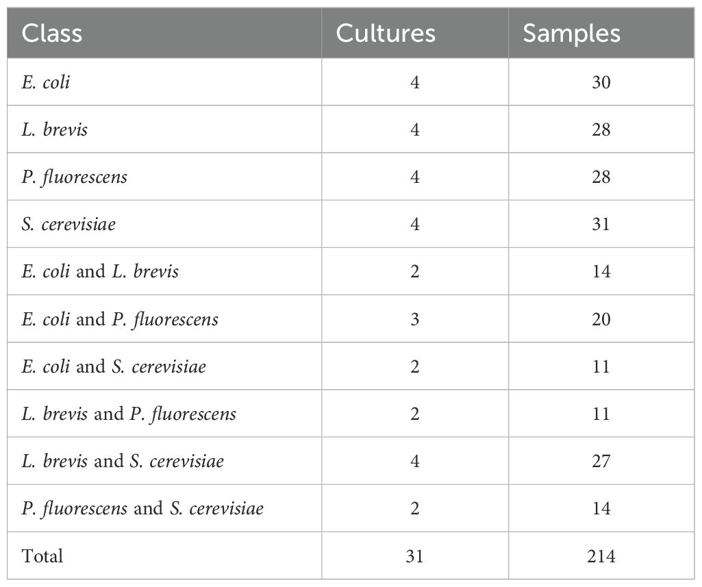
Table 1. Table of cultures and samples for each different class of the dataset.

As shown in Figure 1, a representative GC-IMS spectrum can be visualized as a heatmap, where the x-axis indicates the drift time of the separated ions based on IMS and the y-axis represents the retention time derived by GC, corresponding to the separation characteristics of the sample. The color bar indicates the ion intensity, with specific ions (i.e., VOCs fingerprints) forming peaks at particular coordinates, generating rich informational spectra for analysis.

Figure 1

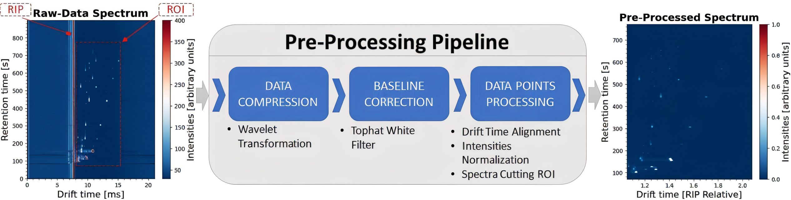
Figure 1. Pre-processing pipeline.

Given the high dimensionality of the input data (3,150 × 6,123), a standard procedure involves applying a pre-processing pipeline (illustrated in Figure 1) to reduce data size, denoise spectra, and extract the most relevant information. To this end, we utilize the open-source Python package gc-ims-tools (Christmann et al., 2022), in accordance to the dataset’s initial publication (Christmann et al., 2024). First, we apply a third-degree wavelet transformation to both the drift and retention time axes, significantly reducing the dimensionality of the spectra to one-tenth of the original data to each direction. Then, a baseline correction algorithm is applied to remove instrumental variations or background noise, using a white top-hat filter of size 15. Finally, to properly prepare the input data for the models, we apply various data points processing techniques. Drift Time Alignment adjusts the drift time axis relative to the Reactant Ion Peak (RIP), which is a standard technique for the task, due to instrumentation variations. Intensities Normalization between zero and one, is a common technique for efficiently training ML and DL models. While, Spectra Cutting is applied on the Region of Interest (ROI), which contains the most valuable information selecting the RIP-relative drift time range between 1.05 and 2.10 and the retention time between 70 and 780 s. The output of the pre-processing pipeline is shown in Figure 1, where the spectral shape is reduced to (152 × 600), resulting in a significant 99.5% reduction in data size.

2.2 Classification methods

As outlined in Section 1, GC-IMS has emerged as a promising tool in various tasks for analyzing samples, particularly in food authentication. DL models have also shown great potential in training effective classifiers based on GC-IMS data. However, limited work has addressed the challenge of identifying bacterial cultures directly from data produced by GC-IMS prototypes. To address this, we employ eight different classification methods, widely used in chemometrics, including four ML models, PLS_DA (Christmann et al., 2024), PCA_LR (Vega-Márquez et al., 2020), PCA_SVM (Vega-Márquez et al., 2020), and XGBoost (Vega-Márquez et al., 2020), and four DL models, FCNN (Vega-Márquez et al., 2020), MLP (Vega-Márquez et al., 2020), CNN1D (Yan et al., 2024), and CNN2D (Yan et al., 2024).

Classical ML models are widely employed by researchers to address a variety of problems. Their main advantages include strong generalization on small datasets, fast training times, and relatively few parameters. PLS_DA is a commonly adopted method in chemometrics, providing both data compression and classification of input spectra. Similarly, PCA combined with either SVM or LR is frequently utilized, benefiting from PCA’s dimensionality reduction capabilities alongside the efficiency of SVM and LR. Additionally, XGBoost is included in our experiments due to its strong performance across a wide range of ML tasks. To ensure reproducibility of results, a random seed of 42 is set during all trainings. For dimensionality reduction, we retain a number of 50 components, while classification models (SVM, LR, XGBoost) are trained using their default hyper-parameters of their respective packages.

In contrast, DL models feature more parameters, longer training times, and more complex architectures. While they require larger datasets, they effectively capture correlations within input parameters, resulting in improved generalization and higher accuracy. We employ CNN2D to capture the spatial structure of the heatmaps, and CNN1D to assess the performance of convolutional layers on flattened heatmaps. Additionally, we include FCNN and MLP as standard baselines for DL-based methods. Figure 2 illustrates the four architectures: CNN2D (Figure 2A), CNN1D (Figure 2B), MLP (Figure 2C), and FCNN (Figure 2C).

Figure 2

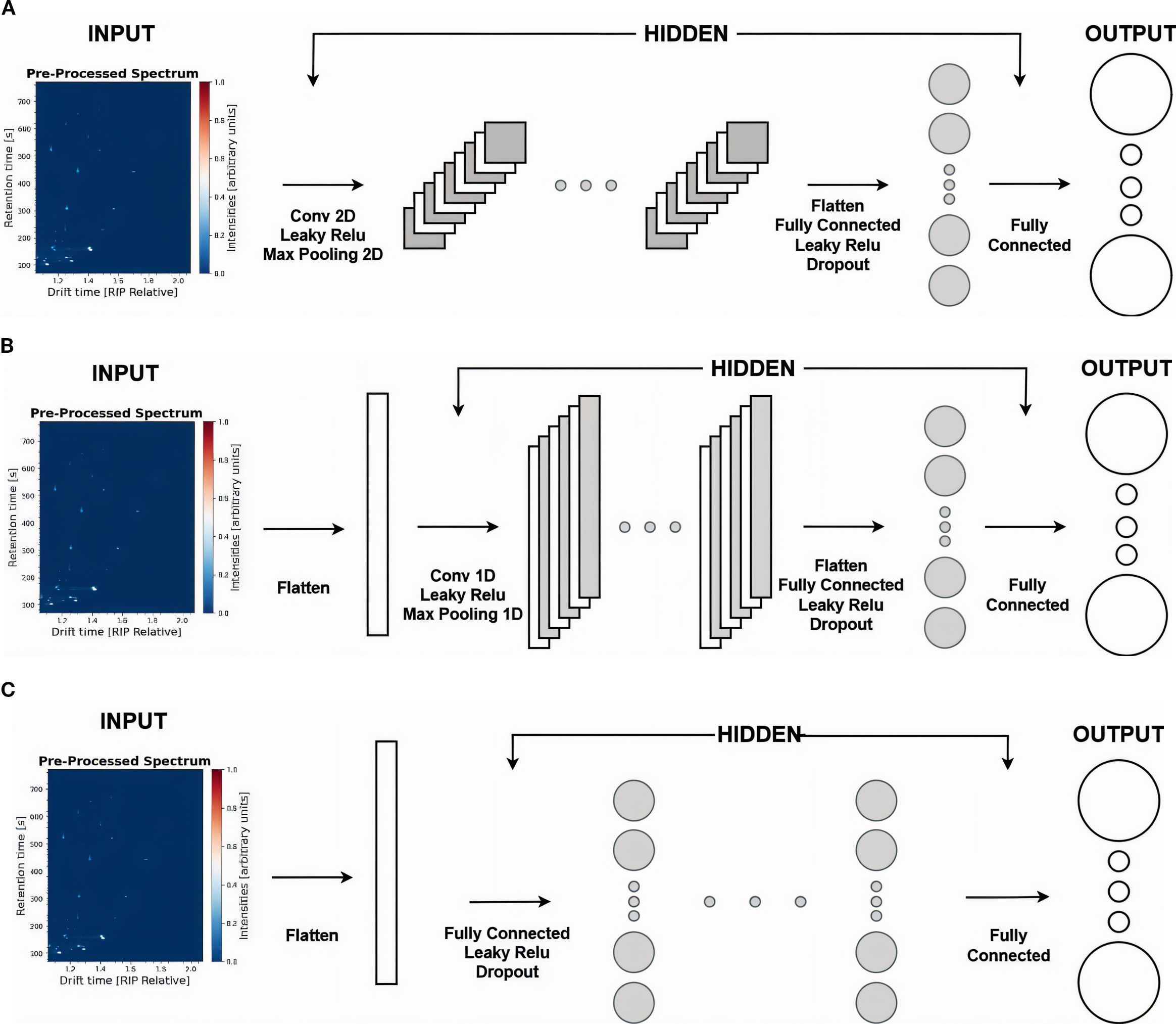
Figure 2. Presentation of four different DL models. (A) Architecture of CNN2D model. (B) Architecture of CNN1D model. (C) Architecture of MLP and FCNN models. Their key difference is the depth of the hidden layers, where on the MLP, we employ a single hidden layer, while on FCNN, we stack four consecutive hidden layers.

The first model, CNN2D (2A), is adopted to leverage the spatial information within the spectra. The pre-processed spectra serve as input to the architecture, which consists of three hidden 2D convolutional layers with a 3×3 kernel size and an increasing number of filters, 32, 64, and 128, respectively. Each convolutional layer is followed by a Leaky ReLU activation and a 2×2 Max Pooling operation. The output of the final convolutional layer is flattened and passed through a fully connected hidden layer with Leaky ReLU activation and a Dropout rate of 0.5, resulting in 512 features. Lastly, a final fully connected layer is applied in the extracted features to generate the target classes.

Additionally, we implement a CNN1D (2B) model. After flattening the input spectra, and following the design of CNN2D (2A), we apply three 1D convolutional layers with a kernel size of 9, each followed by a Leaky ReLU activation and a 1D Max Pooling layer of size 4. The number of filters increases progressively (32, 64, 128). As previously, the output of the final convolutional layer is flattened and passed through a fully connected layer with Leaky ReLU activation and a Dropout rate of 0.5, resulting in 512 features. Finally, a fully connected output layer maps these features to the target classes.

Finally, we employ two models: MLP (2C) and FCNN (2C). In both, the input spectra are flattened and passed through fully connected hidden layers, each followed by a Leaky ReLU activation and a Dropout rate of 0.5, resulting in 512 features. Although their architecture is presented in the same way, the MLP model consists of a single hidden layer, whereas the FCNN model includes four hidden layers, resulting in more parameters and higher complexity. As in the previous models, a final fully connected layer processes these features to generate the target class predictions.

2.3 Evaluation protocol

The original study that introduced this dataset evaluated models using a fixed train/test split. While this approach is common for large datasets, it has significant disadvantages in the context of small datasets like ours. First, with limited samples, a single split can lead to severe under-representation of certain classes in the test set, causing performance metrics to vary greatly depending on which samples are chosen. Second, the original paper does not provide sufficient details regarding how the split was constructed (e.g., sample or culture stratification, class balance, random seed), making it impossible to reproduce the original results and perform a fair, like-for-like comparison. To this end, and given the small number of samples available in the dataset for many classes (see Tables 1, 2), creating a fixed test set would result in under-representation of several classes and make final performance metrics highly sensitive to the specific samples selected.

Table 2

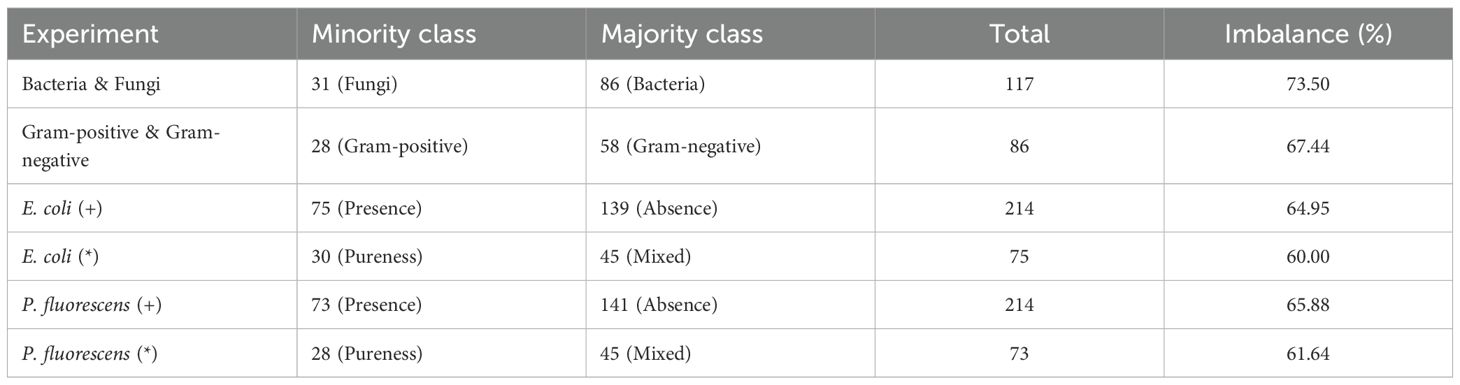
Table 2. Dataset imbalance report.

An alternative strategy that could prevent potential data leakage caused by culture-specific information is Leave-One-Culture-Out (LOCO) cross-validation, where all spectra from a given culture are held out for validation in each iteration. This would provide a rigorous assessment of generalization to unseen cultures. However, our dataset contains only 31 cultures, with as few as 2–4 cultures per class. Under these conditions, LOCO would result in extremely small training sets for some classes (2 cultures in a class, result in 50% split training and validation sets), leading to unstable performance estimates and impractical model training.

To overcome these limitations, we adopt a stratified five-fold cross-validation protocol at the sample level, as illustrated in Figure 3. Cross-Validation is widely recommended for small datasets to improve robustness and reduce variance caused by test set selection, not only in ML and DL in general (Kohavi, 1995; Refaeilzadeh et al., 2009; Raschka, 2018), but also has been widely adopted in chemometrics and bioinformatics tasks for similar reasons (Beleites and Salzer, 2008; Esbensen and Geladi, 2010; Westad and Marini, 2015). In this setup, the dataset is randomly partitioned into five folds while preserving the overall class distribution in each fold. For each iteration, 80% of the samples are used for training and 20% for validation, ensuring that every sample appears exactly once in a validation set across five independent trainings. This approach maximizes the use of available data while maintaining comparability across experiments. To ensure fairness and like-to-like comparison between the proposed methods and the original study’s baselines, we include the PLS_DA model in our evaluation using the same hyperparameters. For reproducibility, all experiments are performed with a fixed random seed of 42.

Figure 3

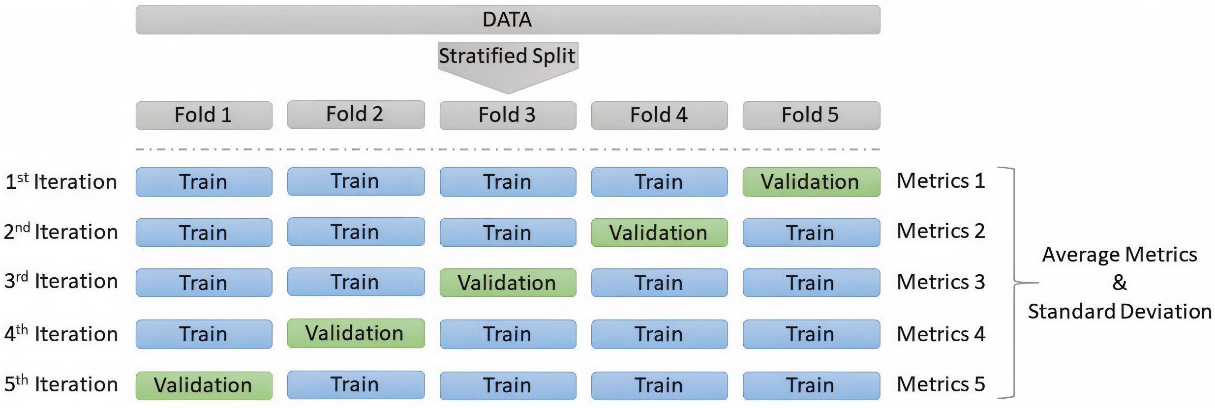
Figure 3. Presentation of five-fold cross-validation evaluation protocol.

For DL baseline models, we employ an Adam optimizer, a learning rate of 0.001, a batch size of 8 and cross-entropy loss function (L_CE), as shown in Equation 1. Although hyperparameter fine-tuning could potentially improve the performance of each individual model, it was not applied in this study due to the limited dataset size and the primary objective of comparing baseline architectures rather than optimizing them, this would be out of scope for this study. Therefore, we report results using standard training hyperparameters.

During training, we evaluate through Accuracy (Equation 2) and F1-score (Equations 3–5) across the validation set, while Sensitivity (Equation 6) and Specificity (Equation 7) are also reported for the validation set for each class c, separately. Additionally, training and inference times along with the number of parameters are reported to provide a comprehensive comparison of each model for each experiment. In the following equations, C, N, TP, TN, FP, and FN represent number of classes, number of samples, true positives, true negatives, false positives, and false negatives, respectively. Moreover, $y_{i,c}$ represent the one-hot encoded ground truth label for sample i and class c, and ${\widehat{y}}_{i,c}$ represent the predicted probability (from softmax) for sample i and class c.

$\begin{array}{ll}{\text{L}}_{CE}=-\frac{1}{N}\sum _{i=1}^N\sum _{c=1}^C{y}_{i,c}\log ({\widehat{y}}_{i,c})& (1)\end{array}$

$\begin{array}{ll}\text{Accuracy}=\frac{TP+TN}{TP+TN+FP+FN}& (2)\end{array}$

$\begin{array}{ll}\text{Precision}=\frac{TP}{TP+FP}& (3)\end{array}$

$\begin{array}{ll}\text{Recall}=\frac{TP}{TP+FN}& (4)\end{array}$

$\begin{array}{ll}\text{F}1-\text{score}=2\times \frac{\text{Precision}\times \text{Recall}}{\text{Precision}+\text{Recall}}& (5)\end{array}$

$\begin{array}{ll}{\text{Sensitivity}}_c=\frac{T{P}_c}{T{P}_c+F{N}_c},\forall c\in \{1,\dots ,C\}& (6)\end{array}$

$\begin{array}{ll}{\text{Specificity}}_c=\frac{T{N}_c}{T{N}_c+F{P}_c},\forall c\in \{1,\dots ,C\}& (7)\end{array}$

2.4 Software and hardware requirements

For the needs of the given research, we conducted all the experiments on a server equipped with a NVIDIA GeForce RTX 4090 GPU. CUDA (12.0) along with Python (3.8.20) have been used, while various packages have been employed among gc-ims-tools (0.1.7) for the data pre-processing pipeline and PLS_DA training, scikit-learn (1.3.2) for the ML models of PCA_SVM and PCA_LR, xgboost (2.1.1) for the XGBoost model and torch (2.4.1+cu118) for the training of DL models.

3 Results

3.1 Tables of experiments

Following, on Tables 3, 4, we present a list of the eight different experiments conducted on the dataset. More precisely, on Table 3, we present two multi-class classification experiments, Pure and Pure & Mixed. As their names suggest, in the first experiment, we train models to classify between the four pure classes, whereas in the second, we train models to classify both pure and mixed cultures, resulting in ten different classes. The numbers indicate the assigned class labels, a standard approach in ML and DL training. Diving deeper into the classification of the pure cultures, we conduct two additional classification experiments, Bacteria & Fungi and Gram-positive & Gram-negative (Table 3). The Bacteria & Fungi experiment is particularly important as it evaluates the models’ ability to distinguish bacterial from fungal behavior. Meanwhile, the Gram-positive & Gram-negative experiment focuses into bacterial characteristics, analyzing their GC-IMS fingerprints based on their cell wall type. These two experiments demonstrate a dataset imbalance, as reported in Table 2, which is a common issue in the literature when training ML and DL models. The Gram-positive class contains 28 samples, while the Gram-negative class has more than twice as many, with 58 samples. Similarly, bacterial samples account for a subset of 86 spectra, whereas fungal samples are limited to just 31, approximately one third.

Table 3

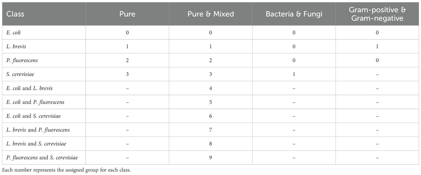
Table 3. Table of experiments categorized by pure, pure & mixed, bacteria & fungi, and Gram-positive & Gram-negative.

Table 4

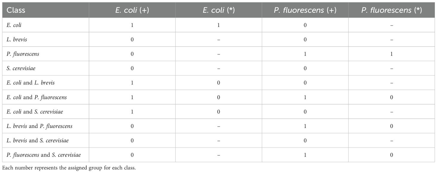
Table 4. Table of experiments regarding the presence (+) and pureness (*) of E. coli and P. fluorescens to specifically identify pathogenic bacterial cultures.

On the other hand, we explore the possibility of specifically identifying either the Presence (+) or the Pureness (*) of two distinct pathogenic bacteria, E. coli and P. fluorescens. As presented in Table 4, to properly evaluate the models’ ability to detect the presence of a specific bacterium, we assign a value of 1 (one) to all the classes containing the given bacteria and 0 (zero) to all the remaining classes. Subsequently, by training from-scratch the models, we investigate their ability to identify the pureness of the bacteria among all the classes in which it is present. This experiment highlights the models’ sensitivity on the given bacteria. These two rounds of experiments are conducted for each bacteria, serving as a baseline for identifying pathogenic bacteria using ML and DL methods based on GC-IMS spectra. Similarly, dataset imbalance is also observed in these experiments (Table 2). For the E. coli (+) experiment, the dataset includes 75 samples with presence and 139 with absence. In the E. coli (*) experiment, results are reported for 30 pure samples and 45 mixed samples. Likewise, for P. fluorescens (+), there are 73 samples with presence and 141 with absence, while the P. fluorescens (*) experiment includes 28 pure samples and 45 mixed samples.

3.2 Pure and mixed cultures

As discussed earlier and in line with the initial dataset’s publication, we experiment with multi-class classification in two different scenarios: Pure and Pure & Mixed cultures. In the Pure experiment, we classify samples into four distinct categories, each representing a pure culture of a specific organism: E. coli, L. brevis, P. fluorescens, and S. cerevisiae. In contrast, the Pure & Mixed experiment evaluates the models’ ability to identify between pure cultures and all possible pairwise mixed cultures in the dataset, resulting in ten distinct classes.

Table 5 presents the classification results for the models described in Subsection 2.2, reporting the average and standard deviation of Accuracy and F1-Score across five cross-validation folds. The highest-performing model is highlighted in bold, while the second-best is underlined. In both experiments, the FCNN model demonstrates clear superiority, achieving 93.19% average accuracy and 93.04% average F1-score in the Pure experiment, and 92.53% average accuracy and 93.37% average F1-score in the Pure & Mixed experiment, all with a relatively small standard deviation. The CNN2D model consistently ranks second, demonstrating strong performance across all metrics and tasks, showcasing its ability to generalize the information based on their spatial information. The overall performance of DL models can be summarized as an out-performance compared to traditional ML baselines.

Table 5

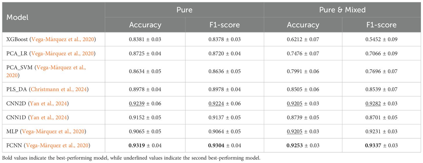
Table 5. Average and standard deviation of accuracy and F1-score for pure and pure & mixed experiments.

Following Table 6, we analyze the Selectivity and Specificity of each class in both experiments using the best-performing model, FCNN. We observe that in both cases, the model achieves strong performance across all classes for both metrics. More specifically, introducing pairwise mixed cultures into the training set affects the performance on pure classes. For instance, the model’s ability to identify E. coli and L. brevis significantly decreases, whereas P. fluorescens and S. cerevisiae maintain or slightly improve their performance. On the other hand, the mixed cultures exhibit a sensitivity variation of up to 10%, while specificity remains consistently high, with differences of less than 1% between values across the different classes.

Table 6

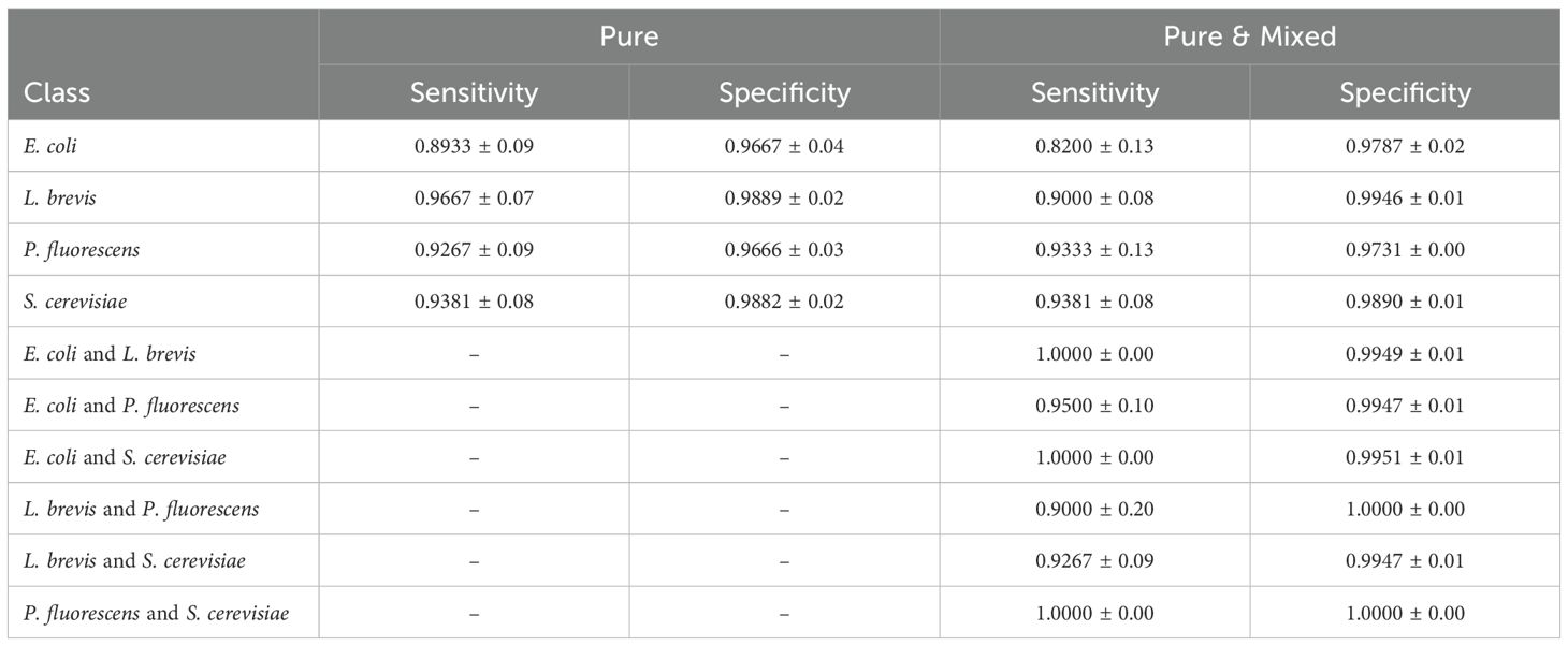
Table 6. Sensitivity and specificity for each class of the best performing model FCNN in pure and pure & mixed experiments.

3.3 Bacteria & Fungi and Gram-positive & Gram-negative

The classification between Bacteria & Fungi is a key experiment in our work, as it highlights the distinct correlations associated with bacterial compared to fungal cultures. In this experiment, we conducted a new training of the models based on their ability to classify between the two categories. The main challenge lies in effectively grouping all bacterial samples and identifying their correlations in comparison to fungi cultures.

As shown in Table 7, both MLP and FCNN models achieve top performance, reaching an average accuracy and f1-score of 98.30% and 97.63%, respectively. These are followed by the other two DL baselines, CNN1D and CNN2D, while the ML baselines also demonstrate promising performance. Similarly, in Table 8, we observe that for class zero (bacteria), the top-performing models achieve 100% sensitivity and 93.33% specificity, with an inverse pattern observed for class one (fungi).

Table 7

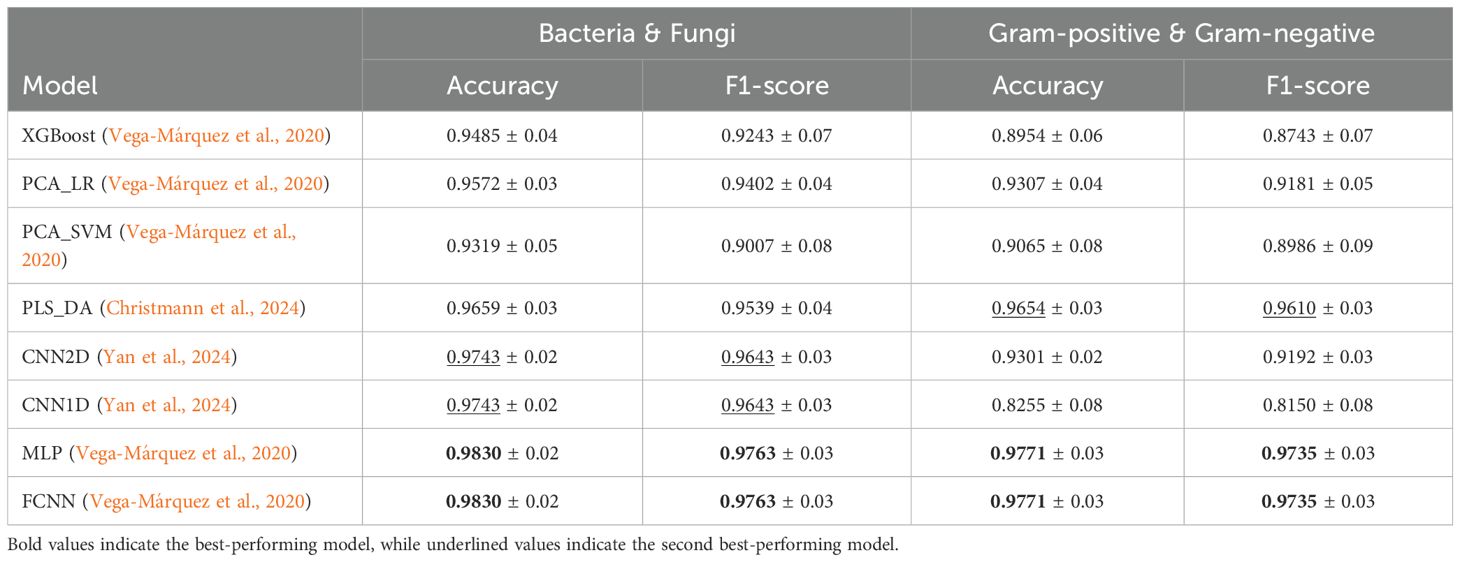
Table 7. Average and standard deviation of Accuracy and F1-score for Bacteria & Fungi and Gram-positive & Gram-negative experiments.

Following the same setup, we conducted another innovative experiment, aiming to further analyze the behavior of a more precise bacterial categorization, namely Gram-positive & Gram-negative. To this end, we assigned class zero to Gram-negative bacteria, including E. coli and P. fluorescens, and class one to Gram-positive bacteria such as L. brevis.

In this task, as shown in Table 7, MLP and FCNN again emerge as the top-performing models, achieving 97.71% accuracy and 97.35% f1-score. The ML baseline PLS_DA follows as the second-best performer in both metrics, while the remaining ML and DL baselines demonstrate significant lower performance. For the best-performing models, FCNN and MLP, sensitivity and specificity alternate between 100% and 93.33% across the two classes, as presented in Table 8.

Table 8

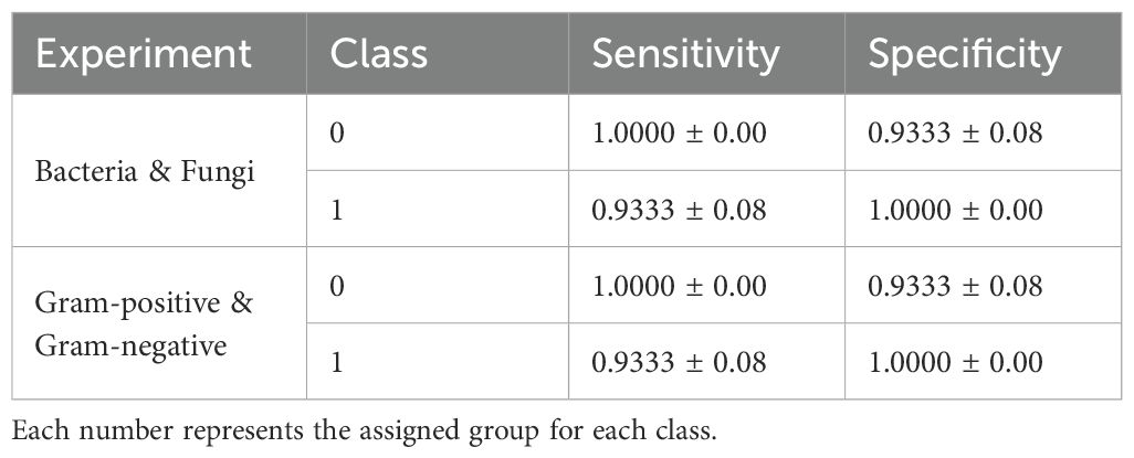
Table 8. Sensitivity and Specificity for each class of the best performing models MLP and FCNN in Bacteria (zero) & Fungi (one) and Gram-positive (one) & Gram-negative (zero) experiments.

3.4 Identification of pathogenic bacterial cultures

Finally, we evaluate the performance of the proposed models in the task of specifically identifying pathogenic bacteria, such as E. coli, as a highly pathogenic bacterium and P. fluorescens as a low pathogenic bacterium. To this end, our initial experiments involve ten different pure and mixed cultures to evaluate the models’ ability to detect the Presence (+) of a specific bacterium. We assign class zero to cultures that do not contain the specific bacterium and class one to those where it is present. Furthermore, among the cultures where the bacterium is present, we further classify the Pureness (*) of the culture in comparison to mixed ones, to dive deeper into the identification of pathogenic bacterial cultures.

As presented in Tables 9, 10, we observe that FCNN is the best-performing model for identifying the presence of E. coli, achieving 92.50% accuracy and an F1-score of 91.40%, closely followed by MLP with 92.04% accuracy and 90.86% F1-score. The remaining baselines exhibit lower performance. Sensitivity and specificity alternate between 96.45% and 84.76%, demonstrating that the model is highly specific in detecting the presence of pathogenic bacteria.

Table 9

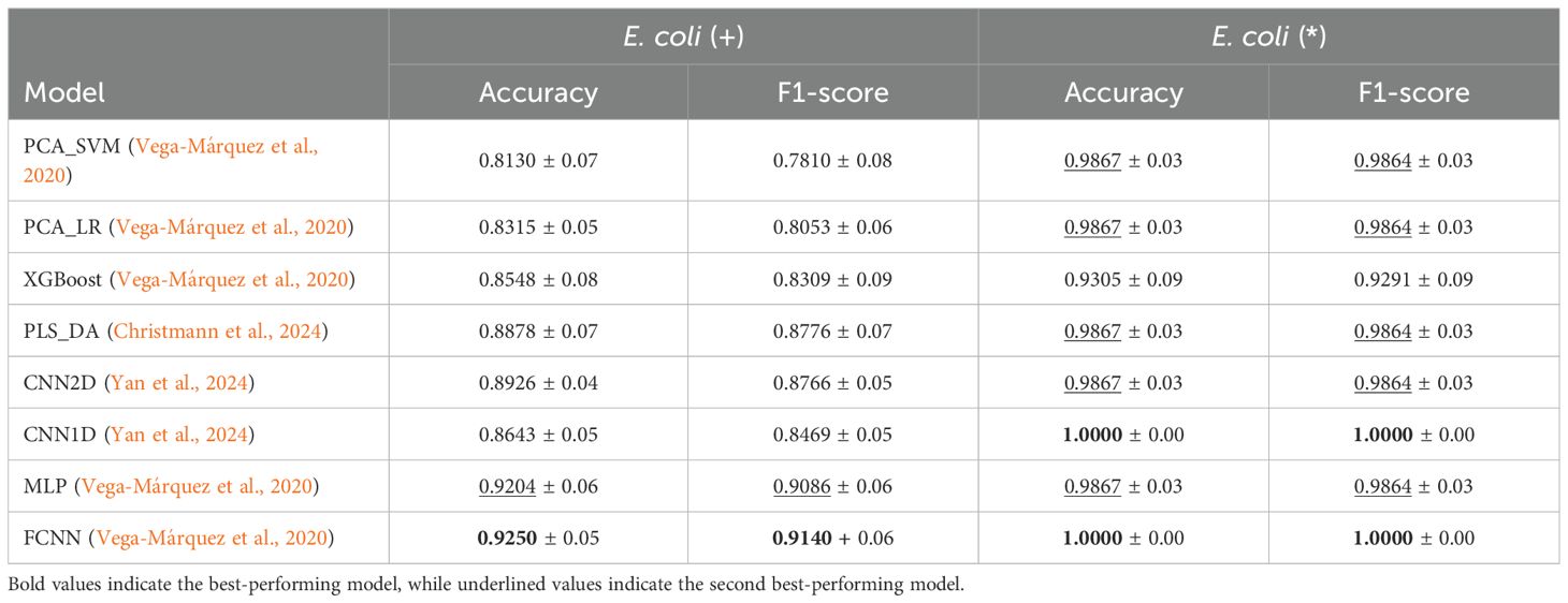
Table 9. Average and standard deviation of Accuracy and F1-score for Presence (+) and Pureness (*) of E. coli experiments.

Table 10

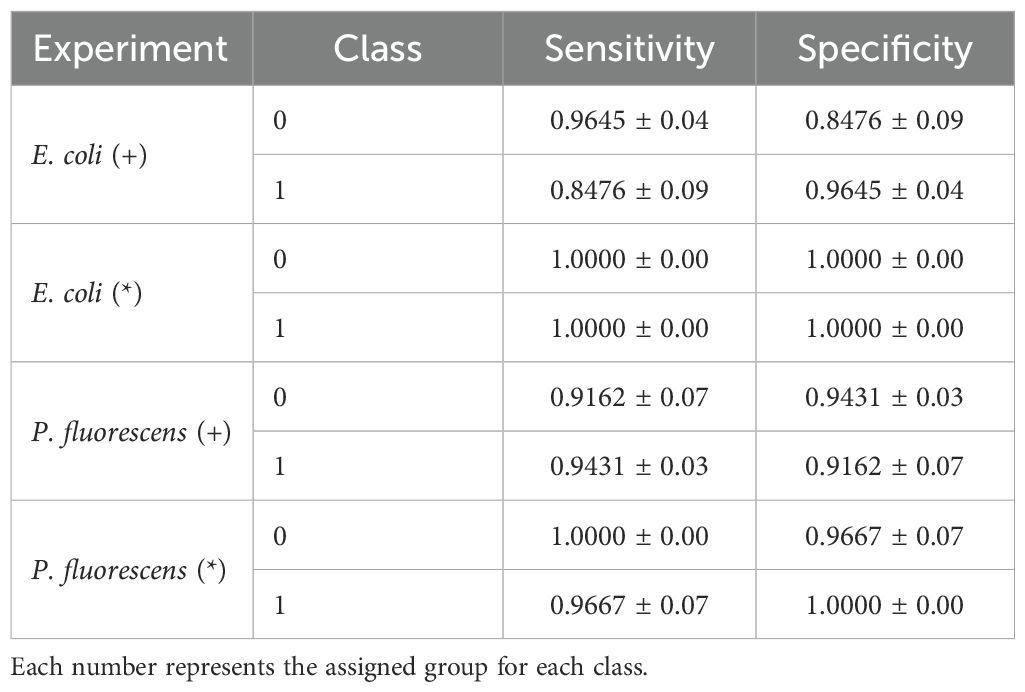
Table 10. Sensitivity and Specificity for each class of the best performing model FCNN in Presence (+) and Pureness (*) of E. coli and P. fluorescens experiments.

On the other hand, when distinguishing between pure and mixed cultures of the pathogenic bacterium E. coli, both FCNN and CNN1D achieved perfect performance, with 100% accuracy, F1-score, sensitivity, and specificity. The remaining baseline models also demonstrated strong performance, further supporting the reliability of the classification. These results highlight the models’ ability to accurately determine the pureness of specific pathogenic bacterial cultures. However, potential dataset-specific or culture-dependent noise should be considered when interpreting these perfect scores. Future work should involve evaluating these classes on larger and more diverse datasets to assess the consistency and generalization of the models.

In alignment with previous experiments, we investigate the classification performance of the models based on the Presence (+) and Pureness (*) of another pathogenic bacterium, P. fluorescens. Table 11 once again highlights the superiority of the FCNN model in both tasks. Specifically, FCNN achieves 93.44% accuracy and an f1-score of 92.70% in the P. fluorescens (+) experiment, followed by MLP and CNN2D, while CNN1D and PLS_DA also demonstrate promising results. Similarly, in the P. fluorescens (*) experiment, FCNN outperforms the other baselines, achieving 98.67% and 98.56% of accuracy and f1-score, respectively. CNN2D follows closely in performance, whereas the remaining baselines exhibit significantly lower results in comparison.

Table 11

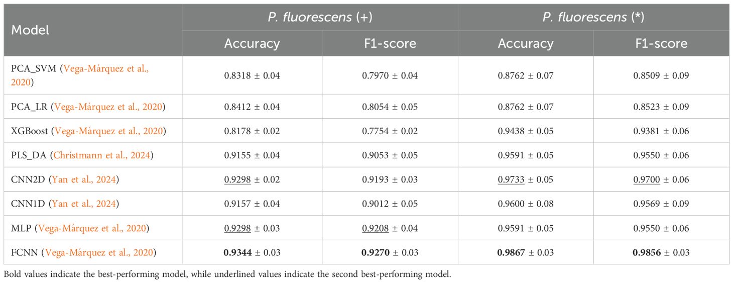
Table 11. Average and standard deviation of Accuracy and F1-score for Presence (+) and Pureness (*) of P. fluorescens experiments.

As shown in Table 10, the sensitivity and specificity of the best-performing model, FCNN, are smoother compared to previous experiments. The values for the two classes in each experiment alternate between 91.62% and 94.31% for the presence of the pathogenic bacterium and between 100% and 96.67% for the pureness of the culture. These findings demonstrate that the models are highly specific in detecting the pureness of the pathogenic bacterium P. fluorescens.

3.5 Evaluation of DL models’ training time and parameters

To further evaluate the proposed DL baseline models, we further report two key evaluation aspects of DL research. First, we measured the training time for each of the four models: CNN1D, CNN2D, MLP, and FCNN. For each experiment and each iteration of the five-fold cross-validation evaluation method, we recorded the overall training time, compute the average and standard deviation in seconds, and presented the results in Table 12.

Table 12

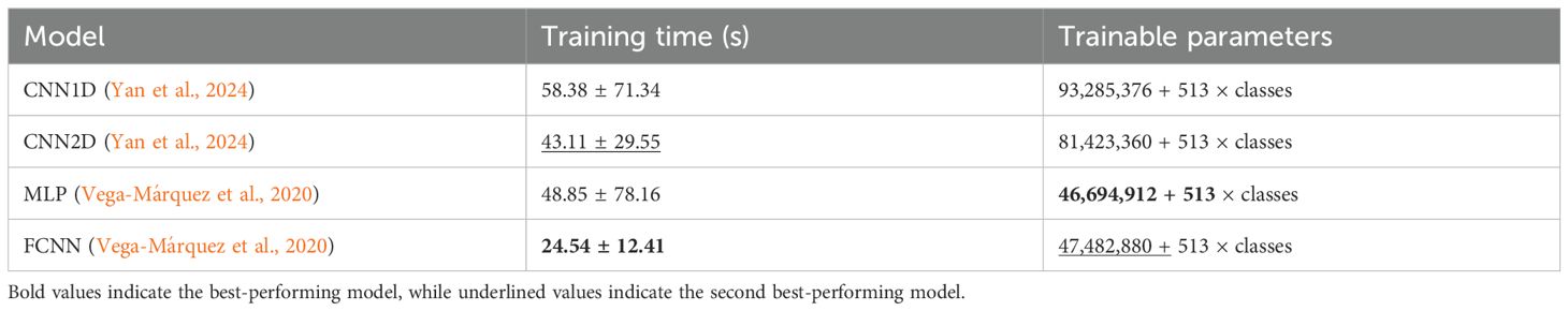
Table 12. Average and standard deviation of training time (s) across all the experiments and number of trainable parameters in respect to the target classes for each DL model.

Notably, FCNN, apart from being the best-performing model across all experiments, exhibited the fastest training time, averaging 24.54 seconds. This is nearly half the time required by the second-fastest model, CNN2D, which averaged 43.11 seconds. MLP followed with an average training time of 48.85 seconds but showed a high standard deviation of 78.16 seconds, and CNN1D had the longest training time, averaging 58.38 ± 71.34 seconds.

Additionally, Table 12 reports the overall number of trainable parameters relative to the number of target classes, as the last hidden layer’s parameters depend on the output classes, as illustrated in Figure 2. MLP has the fewest trainable parameters at 46,694,912, closely followed by FCNN with 47,482,880 parameters, presenting only a 1.68% increase. CNN2D nearly doubles this amount with 81,423,360 parameters, while CNN1D has the highest number, requiring 93,285,376 trainable parameters.

These results highlight that FCNN not only achieves the highest accuracy across all experiments but also is trained fastest and is the second most compact model in terms of trainable parameters. MLP and CNN2D perform competitively depending on the experiment, while CNN1D consistently ranks as the least effective model among the four DL baselines, showcasing that CNN models are quite computationally insufficient in the presented tasks.

4 Discussion

This study explored the ability of ML-based and DL-based supervised classification methods in identifying organism-level microbial cultures through their representative VOCs fingerprints. We investigated pure and mixed cultures of four different microorganisms as multi-class classification problems. Additionally, we introduced two new experiments, one identifying between Bacteria and Fungi, while the other distinguishing Gram-positive from Gram-negative bacteria. Finally, we presented the results on identifying two pathogenic bacteria, Escherichia coli (highly pathogenic) and Pseudomonas fluorescens (low pathogenic), by training models to classify their presence and pureness in various cultures.

To properly evaluate on those experiments, we designed a five-fold cross-validation evaluation protocol for eight different models (PLS_DA, PCA_SVM, PCA_LR, XGBoost, CNN1D, CNN2D, MLP, FCNN), while reporting a wide collection of evaluation metrics. A further evaluation of DL models is conducted to analyze training time and trainable parameters. Based on the reported results, FCNN outperforms the other experimented baselines by achieving the best performance among the models evaluated in this study in terms of overall performance metrics and training time across all experiments, while having a slightly higher parameters count (less than 2%), compared to the lightest model, MLP.

In future work, we plan to incorporate imbalance-aware techniques such as class-weighted losses or focal loss for deep learning models, class weights for machine learning models, and expand the evaluation with metrics like macro-F1, PR-AUC, and 95% confidence intervals computed via bootstrapping across folds to improve and evaluate the models under imbalanced conditions. We also aim to integrate model interpretability methods, such as Grad-CAM or saliency maps for CNN architectures and SHAP for FCNN models, to highlight informative retention-time and drift-time regions, thereby linking predictive features to underlying chemical patterns and ensuring biological plausibility, through various explainable AI techniques.

Finally, due to the significant limitations of the dataset, such as the small number of samples (214 in total) and the imbalance across different experiments, there is a substantial risk of overfitting, which may lead to inflated performance metrics. This limitation makes it difficult to draw definitive conclusions about the generalization capability of our models. While we employed k-fold cross-validation to maximize the use of the limited data in both training and validation sets, we acknowledge that this approach carries a risk of optimistic bias, potential data leakage, or overfitting to instrumentation-specific noise. Therefore, it is important to emphasize that this work represents an early-stage investigation under controlled laboratory conditions and does not constitute clinical validation. To establish real-world applicability, future studies should also include clinically relevant samples processed under different culture media and across multiple GC-IMS instruments and laboratories. A key next step will be the creation of a large-scale, multi-site dataset that incorporates diverse instruments, operators, and sample preparation protocols. Such an effort will be essential to evaluate the robustness, transferability, and generalization of the proposed models.

Data availability statement

The original contributions presented in the study are included in the article/supplementary material. Further inquiries can be directed to the corresponding author.

Author contributions

GK: Writing – original draft, Writing – review & editing, Conceptualization, Data curation, Formal analysis, Investigation, Methodology, Software, Validation, Visualization. GD: Conceptualization, Funding acquisition, Project administration, Resources, Supervision, Validation, Visualization, Writing – original draft, Writing – review & editing. SK: Funding acquisition, Project administration, Writing – review & editing. KI: Funding acquisition, Project administration, Resources, Supervision, Writing – review & editing. SV: Funding acquisition, Project administration, Writing – review & editing. IK: Funding acquisition, Project administration, Writing – review & editing.

Funding

The author(s) declare financial support was received for the research and/or publication of this article. Funded by the European Union through Grant Agreement 101103176.

Conflict of interest

The authors declare that the research was conducted in the absence of any commercial or financial relationships that could be construed as a potential conflict of interest.

The author(s) declared that they were an editorial board member of Frontiers, at the time of submission. This had no impact on the peer review process and the final decision.

Generative AI statement

The author(s) declare that no Generative AI was used in the creation of this manuscript.

Any alternative text (alt text) provided alongside figures in this article has been generated by Frontiers with the support of artificial intelligence and reasonable efforts have been made to ensure accuracy, including review by the authors wherever possible. If you identify any issues, please contact us.

Publisher’s note

All claims expressed in this article are solely those of the authors and do not necessarily represent those of their affiliated organizations, or those of the publisher, the editors and the reviewers. Any product that may be evaluated in this article, or claim that may be made by its manufacturer, is not guaranteed or endorsed by the publisher.

Author disclaimer

Views and opinions expressed are however those of the author(s) only and do not necessarily reflect those of the European Union or the European Commission. Neither the European Union nor the granting authority can be held responsible for them.

References

Aboutalebian S., Ahmadikia K., Fakhim H., Chabavizadeh J., Okhovat A., Nikaeen M., et al. (2021). Direct detection and identification of the most common bacteria and fungi causing otitis externa by a stepwise multiplex pcr. Front. Cell. Infect. Microbiol. 11, 644060. doi: 10.3389/fcimb.2021.644060

PubMed Abstract | Crossref Full Text | Google Scholar

Altaee N., Kadhim M. J., and Hameed I. H. (2017). Characterization of metabolites produced by e. coli and analysis of its chemical compounds using gc-ms. Int. J. Curr. Pharm. Rev. Res. 7, 13–19.

Google Scholar

Baron S. (1996). Introduction to bacteriology. BMJ 2, 245–245. doi: 10.1136/bmj.2.5351.245

Crossref Full Text | Google Scholar

Beleites C. and Salzer R. (2008). Assessing and improving the stability of chemometric models in small sample size situations. Analytical. Bioanal. Chem. 390, 1261–1271. doi: 10.1007/s00216-007-1818-6

PubMed Abstract | Crossref Full Text | Google Scholar

Chauhan A. and Jindal T. (2020). “Biochemical and molecular methods for bacterial identification,” in Microbiological methods for environment, food and pharmaceutical analysis Cham: Springer International Publishing, 425–468. doi: 10.1007/978-3-030-52024-3_10

Crossref Full Text | Google Scholar

Christmann J., Rohn S., and Weller P. (2022). gc-ims-tools–a new python package for chemometric analysis of gc–ims data. Food Chem. 394, 133476. doi: 10.1016/j.foodchem.2022.133476

PubMed Abstract | Crossref Full Text | Google Scholar

Christmann J., Weber M., Rohn S., and Weller P. (2024). Nontargeted volatile metabolite screening and microbial contamination detection in fermentation processes by headspace gc-ims. Analytical. Chem. 96, 3794–3801. doi: 10.1021/acs.analchem.3c04857

PubMed Abstract | Crossref Full Text | Google Scholar

Clark C. G., Kruczkiewicz P., Guan C., McCorrister S. J., Chong P., Wylie J., et al. (2013). Evaluation of maldi-tof mass spectroscopy methods for determination of escherichia coli pathotypes. J. Microbiol. Methods 94, 180–191. doi: 10.1016/j.mimet.2013.06.020

PubMed Abstract | Crossref Full Text | Google Scholar

Dingle T. C. and Butler-Wu S. M. (2013). Maldi-tof mass spectrometry for microorganism identification. Clinics Lab. Med. 33, 589–609. doi: 10.1016/j.cll.2013.03.001

PubMed Abstract | Crossref Full Text | Google Scholar

Drees C., Vautz W., Liedtke S., Rosin C., Althoff K., Lippmann M., et al. (2019). Gc-ims headspace analyses allow early recognition of bacterial growth and rapid pathogen differentiation in standard blood cultures. Appl. Microbiol. Biotechnol. 103, 9091–9101. doi: 10.1007/s00253-019-10181-x

PubMed Abstract | Crossref Full Text | Google Scholar

Duriez E., Armengaud J., Fenaille F., and Ezan E. (2016). Mass spectrometry for the detection of bioterrorism agents: from environmental to clinical applications. J. Mass. Spectromet. 51, 183–199. doi: 10.1002/jms.3747

PubMed Abstract | Crossref Full Text | Google Scholar

Dybwad M., van der Laaken A. L., Blatny J. M., and Paauw A. (2013). Rapid identification of bacillus anthracis spores in suspicious powder samples by using matrix-assisted laser desorption ionization–time of flight mass spectrometry (MALDI-TOF MS). Applied and Environmental Microbiology, 79 (17), 5372–5383. Washington: American Society for Microbiology (ASM).

PubMed Abstract | Google Scholar

Esbensen K. H. and Geladi P. (2010). Principles of proper validation: use and abuse of re-sampling for validation. J. Chemometr. 24, 168–187. doi: 10.1002/cem.1310

Crossref Full Text | Google Scholar

Feng B., Shi L., Zhang H., Shi H., Ding C., Wang P., et al. (2021). Effective discrimination of yersinia pestis and yersinia pseudotuberculosis by maldi-tof ms using multivariate analysis. Talanta 234, 122640. doi: 10.1016/j.talanta.2021.122640

PubMed Abstract | Crossref Full Text | Google Scholar

Gallien S., Duriez E., Crone C., Kellmann M., Moehring T., and Domon B. (2012). Targeted proteomic quantification on quadrupole-orbitrap mass spectrometer. Mol. Cell. Proteomics 11, 1709–1723. doi: 10.1074/mcp.O112.019802

PubMed Abstract | Crossref Full Text | Google Scholar

Gerhardt N., Schwolow S., Rohn S., Pérez-Cacho P. R., Galán-Soldevilla H., Arce L., et al. (2019). Quality assessment of olive oils based on temperature-ramped hs-gc-ims and sensory evaluation: Comparison of different processing approaches by lda, knn, and svm. Food Chem. 278, 720–728. doi: 10.1016/j.foodchem.2018.11.095

PubMed Abstract | Crossref Full Text | Google Scholar

Giuliano C., Patel C. R., and Kale-Pradhan P. B. (2019). Kale-Pradhan PB. A guide to bacterial culture identification and results interpretation. Pharm. Ther. 44, 192.

PubMed Abstract | Google Scholar

Gu S., Zhang J., Wang J., Wang X., and Du D. (2021). Recent development of hs-gc-ims technology in rapid and non-destructive detection of quality and contamination in agri-food products. TrAC. Trends Analytical. Chem. 144, 116435. doi: 10.1016/j.trac.2021.116435

Crossref Full Text | Google Scholar

Hameed R. H., Abbas F. M., and Hameed I. H. (2018). Analysis of secondary metabolites released by pseudomonas fluorescens using gc-ms technique and determination of its anti-fungal activity. Indian J. Public Health Res. Dev. 9, 449–455. doi: 10.5958/0976-5506.2018.00485.0

Crossref Full Text | Google Scholar

Ishii H., Kushima H., Koide Y., and Kinoshita Y. (2024). Pseudomonas fluorescens pneumonia. Int. J. Infect. Dis. 140, 92–94. doi: 10.1016/j.ijid.2024.01.007

PubMed Abstract | Crossref Full Text | Google Scholar

Jeon J. H., Kim J. S., Kim Z. H., and Jung J. Y. (2024). Complete genome sequence of levilactobacillus brevis nsmj23, makgeolli isolate with antimicrobial activity. Microbiol. Resour. Announcements. 13, e01060–e01023. doi: 10.1128/mra.01060-23

PubMed Abstract | Crossref Full Text | Google Scholar

Ju X., Lian F., Ge H., Jiang Y., Zhang Y., and Xu D. (2021). Identification of rice varieties and adulteration using gas chromatography-ion mobility spectrometry. IEEE Access 9, 18222–18234. doi: 10.1109/Access.6287639

Crossref Full Text | Google Scholar

Kim S. O. and Kim S. S. (2021). Bacterial pathogen detection by conventional culture-based and recent alternative (polymerase chain reaction, isothermal amplification, enzyme linked immunosorbent assay, bacteriophage amplification, and gold nanoparticle aggregation) methods in food samples: A review. J. Food Saf. 41, e12870. doi: 10.1111/jfs.12870

Crossref Full Text | Google Scholar

Kirtsanis G., Dolias G., Kintzios S., Ioannidis K., Vrochidis S., and Kompatsiaris I. (2025). “Cnn-based deep autoencoders for limited gas chromatography-ion mobility spectrometry data,” in 2025 IEEE International Instrumentation and Measurement Technology Conference (I2MTC). 1–6 (IEEE). doi: 10.1109/I2MTC62753.2025.11079137

Crossref Full Text | Google Scholar

Kohavi R. (1995). A study of cross-validation and bootstrap for accuracy estimation and model selection Vol. 14 (Montreal, Canada: Ijcai) 14 (2), 1137–1145.

Google Scholar

Lasch P., Drevinek M., Nattermann H., Grunow R., Stammler M., Dieckmann R., et al. (2010). Characterization of yersinia using maldi-tof mass spectrometry and chemometrics. Analytical. Chem. 82, 8464–8475. doi: 10.1021/ac101036s

PubMed Abstract | Crossref Full Text | Google Scholar

Li G., Li S., Fang X., Luan X., and Liu F. (2024). “An improved yolov3 model for detection of invasive saccharomyces cerevisiae infections,” in Multimedia Tools and Applications Cham: Springer International Publishing, 1–18. doi: 10.1007/s11042-024-19649-z

Crossref Full Text | Google Scholar

Lu Y., Zeng L., Li M., Yan B., Gao D., Zhou B., et al. (2022). Use of gc-ims for detection of volatile organic compounds to identify mixed bacterial culture medium. Amb. Express. 12, 31. doi: 10.1186/s13568-022-01367-0

PubMed Abstract | Crossref Full Text | Google Scholar

Nunes A. L., Perna O. F., Queiroz M. S., Zaro G. C., de Lima J. D., and da Silva G. J. (2024). “Role of pseudomonas fluorescens secondary metabolites in agroecosystem applications,” in Bacterial secondary Metabolites (Amsterdam: Elsevier), 211–220. doi: 10.1016/B978-0-323-95251-4.00008-9

Crossref Full Text | Google Scholar

Pohanka M. (2019). Current trends in the biosensors for biological warfare agents assay. Materials 12, 2303. doi: 10.3390/ma12142303

PubMed Abstract | Crossref Full Text | Google Scholar

Raschka S. (2018). Model evaluation, model selection, and algorithm selection in machine learning. arXiv. preprint. arXiv:1811.12808. doi: 10.48550/arXiv.1811.12808

Crossref Full Text | Google Scholar

Refaeilzadeh P., Tang L., and Liu H. (2009). “Cross-validation,” in Encyclopedia of database systems (Boston, MA: Springer), 532–538. doi: 10.1007/978-0-387-39940-9_565

Crossref Full Text | Google Scholar

Rezaei F. Y., Pircheraghi G., and Nikbin V. S. (2024). Antibacterial activity, cell wall damage, and cytotoxicity of zinc oxide nanospheres, nanorods, and nanoflowers. ACS Appl. Nano. Mater. 7, 15242–15254. doi: 10.1021/acsanm.4c02046

Crossref Full Text | Google Scholar

Sauer S. and Kliem M. (2010). Mass spectrometry tools for the classification and identification of bacteria. Nat. Rev. Microbiol. 8, 74–82. doi: 10.1038/nrmicro2243

PubMed Abstract | Crossref Full Text | Google Scholar

Su H., Jiang Z. H., Chiou S. F., Shiea J., Wu D. C., Tseng S. P., et al. (2022). Rapid characterization of bacterial lipids with ambient ionization mass spectrometry for species differentiation. Molecules 27, 2772. doi: 10.3390/molecules27092772

PubMed Abstract | Crossref Full Text | Google Scholar

Tait E., Perry J. D., Stanforth S. P., and Dean J. R. (2014). Identification of volatile organic compounds produced by bacteria using hs-spme-gc–ms. J. Chromatogr. Sci. 52, 363–373. doi: 10.1093/chromsci/bmt042

PubMed Abstract | Crossref Full Text | Google Scholar

Vega-Márquez B., Nepomuceno-Chamorro I., Jurado-Campos N., and Rubio-Escudero C. (2020). Deep learning techniques to improve the performance of olive oil classification. Front. Chem. 7, 929. doi: 10.3389/fchem.2019.00929

PubMed Abstract | Crossref Full Text | Google Scholar

Wang R. Y., Yan Y. Y., Li B., Fan X., Gu B., Zhou Y., et al. (2023). Pattern recognition analysis of metabolites in escherichia coli based on esi-orbitrap mass spectrometry. Chem. Biodivers. 20, e202201153. doi: 10.1002/cbdv.202201153

PubMed Abstract | Crossref Full Text | Google Scholar

Wang S., Chen H., and Sun B. (2020). Recent progress in food flavor analysis using gas chromatography–ion mobility spectrometry (gc–ims). Food Chem. 315, 126158. doi: 10.1016/j.foodchem.2019.126158

PubMed Abstract | Crossref Full Text | Google Scholar

Weller P. and Christmann J. (2023). Hs-gc-ims data of fermentations of different organisms. Mendeley Data, V1. doi: 10.17632/v9gxkpdp3c.1

Crossref Full Text | Google Scholar

Westad F. and Marini F. (2015). Validation of chemometric models–a tutorial. Analytica. Chim. Acta 893, 14–24. doi: 10.1016/j.aca.2015.06.056

PubMed Abstract | Crossref Full Text | Google Scholar

Wynne C., Edwards N. J., and Fenselau C. (2010). Phyloproteomic classification of unsequenced organisms by top-down identification of bacterial proteins using caplc-ms/ms on an orbitrap. Proteomics 10, 3631–3643. doi: 10.1002/pmic.201000172

PubMed Abstract | Crossref Full Text | Google Scholar

Yan B., Zeng L., Lu Y., Li M., Lu W., Zhou B., et al. (2024). Rapid bacterial identification through volatile organic compound analysis and deep learning. BMC Bioinf. 25, 347. doi: 10.1186/s12859-024-05967-4

PubMed Abstract | Crossref Full Text | Google Scholar

Yang S. C., Lin C. H., Aljuffali I. A., and Fang J. Y. (2017). Current pathogenic escherichia coli foodborne outbreak cases and therapy development. Arch. Microbiol. 199, 811–825. doi: 10.1007/s00203-017-1393-y

PubMed Abstract | Crossref Full Text | Google Scholar

Yang M., Wang Z., Su M., Zhu S., Xie Y., and Ying B. (2024). Smart nanozymes for diagnosis of bacterial infection: The next frontier from laboratory to bedside testing. ACS Appl. Mater. Interfaces. 16, 44361–44375. doi: 10.1021/acsami.4c07043

PubMed Abstract | Crossref Full Text | Google Scholar

Zhao Z., Lian F., and Jiang Y. (2024). Recognition of rice species based on gas chromatography-ion mobility spectrometry and deep learning. Agriculture 14, 1552. doi: 10.3390/agriculture14091552

Crossref Full Text | Google Scholar

Zukowska M. E. (2021). Advanced methods of bacteriological identification in a clinical microbiology laboratory. J. Pre-Clin. Clin. Res. 15 (2), 68–72. doi: 10.26444/jpccr/134646

Crossref Full Text | Google Scholar