Protein quality assessment with a loss function designed for high-quality decoys

Motivation: The prediction of a protein 3D structure is essential for understanding protein function, drug discovery, and disease mechanisms; with the advent of methods like AlphaFold that are capable of producing very high-quality decoys, ensuring the quality of those decoys can provide further confidence in the accuracy of their predictions.

Results: In this work, we describe Q_ϵ, a graph convolutional network (GCN) that utilizes a minimal set of atom and residue features as inputs to predict the global distance test total score (GDTTS) and local distance difference test (lDDT) score of a decoy. To improve the model’s performance, we introduce a novel loss function based on the ϵ-insensitive loss function used for SVM regression. This loss function is specifically designed for evaluating the characteristics of the quality assessment problem and provides predictions with improved accuracy over standard loss functions used for this task. Despite using only a minimal set of features, it matches the performance of recent state-of-the-art methods like DeepUMQA.

Availability: The code for Q_ϵ is available at https://github.com/soumyadip1997/qepsilon.

1 Introduction

Predicting a protein’s 3D structure from its amino acid sequence has been an area of avid interest for many years (Al-Lazikani et al., 2001). Recently, significant progress has been made in this field with the introduction of AlphaFold, a deep learning system that achieved remarkable accuracy in predicting protein structures (Jumper et al., 2021). While experimental identification of native protein structures remains a time-consuming and costly process, computational methods have made it possible to generate thousands of tertiary structures, known as decoys, in a matter of hours (Shehu, 2015). However, identifying the best structure remains a challenge. Therefore, it is necessary to employ a quality assessment stage to identify high-quality, near-native decoys among the generated decoys (Akhter et al., 2020). This remains true even with AlphaFold’s recent breakthrough performance (Chen et al., 2023). Furthermore, with the subsequent availability of genome-wide predicted structures across many species (Varadi et al., 2022), the quality assessment problem is as relevant as ever.

In this work, we address the decoy quality assessment problem with the help of graph convolutional networks (GCNs); we introduce a novel loss function inspired by the support vector regression, ϵ-insensitive loss function, that is designed to take into account our intuition about what makes a good quality assessment predictor, namely, that it focuses on making correct predictions for those decoys that matter: decoys with high quality. We compare our method, called Q_ϵ, to other state-of-the-art methods and demonstrate that our method outperforms most of those methods while using only a very basic set of features computed from a decoy’s sequence, without the need for engineered features.

2 Related work

Current techniques for quality assessment can be divided into two categories. One is single-model methods that operate on single structural models to estimate their quality (Wallner and Elofsson, 2003). The second category consists of methods that use consistency among several candidates to estimate quality (Lundström et al., 2001). Protein quality assessment methods have been evaluated in the Critical Assessment of Structure Prediction (CASP) competition (Moult et al., 1995) since CASP7. The CASP13 single-model methods, the focus of this work, performed comparably or better than consensus methods for the first time (Cheng et al., 2019). A variety of single-model approaches have been proposed, and currently, machine learning-based methods dominate this area.

Until a few years ago, methods that use standard machine learning techniques with a large collection of engineered features computed from sequence and structure were the prevalent approaches for quality assessment. The ProQ series of methods (ProQ, ProQ2, ProQ3, and ProQ3D) (Uziela et al., 2017) used features such as the distribution of atom–atom contacts, residue–residue contacts, solvent accessibility, secondary structure, surface area, and evolutionary information. ProQ3 (Uziela et al., 2016) also incorporated features based on Rosetta energies. ProQ3D (Uziela et al., 2017) used the descriptors of ProQ3 as inputs in conjunction with a multi-layer perceptron and was one of the top performers of CASP13.

The current state-of-the-art method for quality assessment uses deep learning, including various types of 3D convolutional networks and graph neural networks, which have been demonstrated to be effective tools for modeling protein 3D structures (Derevyanko et al., 2018; Fout et al., 2017). Deep convolutional networks as a tool for the representation of decoy structures were introduced by Derevyanko et al. (2018). Their method, 3DCNN, used 3D convolutional networks applied to a volumetric representation of a decoy structure. The Ornate method by Pagès et al. (2019) improved upon 3DCNN by defining a canonical orientation for each residue. The GraphQA method by Baldassarre et al. (2020) employed a graph convolutional network with an extensive number of engineered features and achieved state-of-the-art performance on CASP13 decoys. Chen et al. (2023) used a graph neural network to estimate the accuracy of AlphaFold models, which is one of the current state-of-the-art methods, and improved on the results obtained with DeepAccNet by Hiranuma et al. (2021) while borrowing many ideas from its architecture. They used a combination of categorical loss and L2-loss on the lDDT scores to distinguish between decoys of varying quality levels. The DeepUMQA method uses 3D convolution over a collection of residue-level engineered features (Guo et al., 2022), and its successor, DeepUMQA2 (Liu et al., 2023), is also a state-of-the-art performer.

Most existing methods for quality assessment rely on engineered features. In contrast, our approach uses sequence embeddings computed using protein language models; convolutional layers applied to both atomic- and residue-level graphs are then used to put them in the context of the decoy structure. In combination with a novel loss function specifically designed for the quality assessment problem, our method can outperform the recent DeepUMQA method (Guo et al., 2022).

3 Methods

3.1 The quality assessment problem

Computational methods for predicting a protein’s 3D structure produce large numbers of decoy conformations for a given target protein. In quality assessment, we seek to rank these decoys based on their similarity to the experimentally determined native structure. We address this as a regression problem: our method is designed to predict the global distance test total score (GDTTS) (Zemla, 2003) and the local distance difference test (lDDT) score (Mariani et al., 2013), which are the official CASP scores for global-level decoy quality. While several recent methods were designed to predict the lDDT score (Hiranuma et al., 2021; Chen et al., 2023), we used both scores to allow for direct comparison with GraphQA, which is the most similar approach to the method presented here and would allow us to compare with more recent QA methods like DeepUMQA and DeepUMQA2. GDTTS measures the percentage of residues in the superimposed predicted structure that are within a certain distance threshold of their corresponding residues in the true structure. lDDT score is a superposition-free score that represents the local distance difference among all atoms in a predicted structure, thereby providing an idea of the local quality of the predicted structure. Decoy structures with high GDTTS and lDDT score ($>$0.85) indicate that they closely resemble the native structure. In what follows, we describe Q_ϵ, a graph convolutional network that is trained on labeled decoy 3D structures, utilizing a basic set of features generated from atoms and residues using a combination of the L1-loss and a modification of the SVM regression ϵ-insensitive loss function (Drucker et al., 1996).

3.2 Atom- and residue-level graph convolution

Graph convolution is a powerful approach for representing protein 3D structures (Fout et al., 2017) and has proven its value for the quality assessment problem (Baldassarre et al., 2020). In order to enable us to forgo engineered features, we have chosen to represent the 3D structure of a decoy using dual graphs at the atom and residue levels (see Figure 1). Each of the graphs is a nearest neighbor graph where a pair of nodes is connected by an edge if their distance in the structure is less than a given threshold, where 6Å was the selected value in our experiments, and the distance between residues is the minimum distance between their atoms. We used up to 20 nearest neighbors to define the edges in both the atom-level and the residue-level graphs.

FIGURE 1

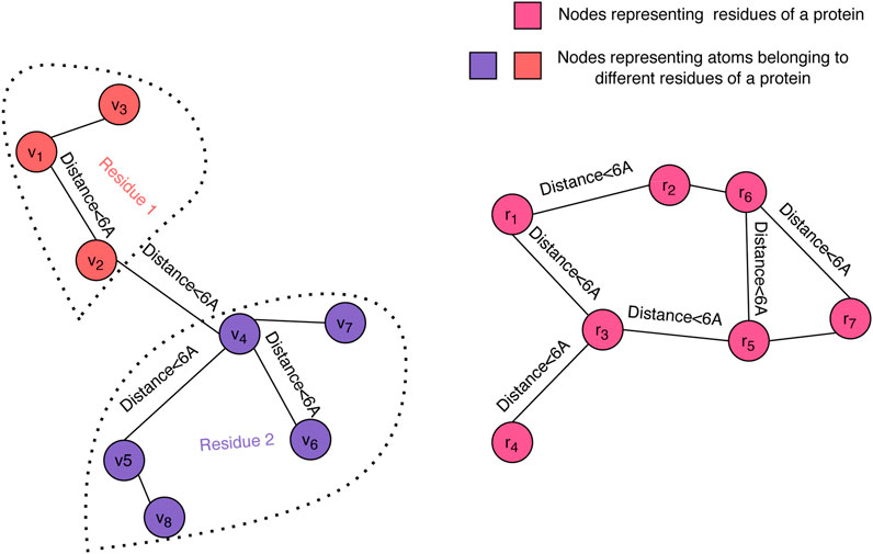
FIGURE 1. Graph representation of a decoy structure. The structure of a decoy is represented using two graphs: one at the atomic level (left) and one at the residue level (right). Our graph convolution operation at the atom level differentiates between edges within a residue and edges across neighboring residues.

We perform graph convolution separately at the atom and residue levels. First, we describe the atom-level graph convolution (GCN_atom). Each atom i is assigned a feature vector ${\mathrm{v}}_i^{(l)}$ that contains the features for layer l of graph convolution. The representation of a source atom ${\mathrm{v}}_i^{(l)}$ is updated based on its neighbors within the same residue $({\mathcal{N}}^{(s)}(i))$ and the neighbors across residues $({\mathcal{N}}^{(o)}(i))$ according to

${\mathrm{v}}_i^{\left(l+1\right)}=\mathrm{R}\mathrm{e}\mathrm{L}\mathrm{U}(W_l^{\left(c\right)}{\mathrm{v}}_i^{\left(l\right)}+\frac{1}{|{\mathcal{N}}^{\left(s\right)}\left(i\right)|}{W}_l^{\left(s\right)}{\displaystyle \sum _{j\in {\mathcal{N}}^{\left(s\right)}\left(i\right)}}{\mathrm{v}}_j^{\left(l\right)}+\frac{1}{|{\mathcal{N}}^{\left(o\right)}\left(i\right)|}{W}_l^{\left(o\right)}{\displaystyle \sum _{j\in {\mathcal{N}}^{\left(o\right)}\left(i\right)}}{\mathrm{v}}_j^{\left(l\right)}+b_v^{\left(l\right)}),(1)$

where $W_l^{(c)}$ is the weight matrix with respect to the source atom in layer l, $W_l^{(s)}$ is the weight matrix with respect to the neighboring atoms in layer l within the same residue as that of the source atom, $W_l^{(o)}$ is the weight matrix with respect to the neighboring atoms in layer l that belong to a different residue than the source atom, and finally, $b_v^{(l)}$ is the bias in layer l for the atom-level GCN. The inputs to the atom-level convolution are derived from one-hot encoding of the atom type as described in the following sections.

In parallel to the atom-level convolution, we perform convolution over the residues that make up a decoy structure. This operation, denoted as GCN_residue, is used to update the residue-level representation ${\mathrm{r}}_i^{(l)}$, which is the feature vector for residue i in layer l of the network. This operation is defined as follows:

${\mathrm{r}}_i^{\left(l+1\right)}=\mathrm{R}\mathrm{e}\mathrm{L}\mathrm{U}\left(W_l^{\left(cr\right)}{\mathrm{r}}_i^{\left(l\right)}+\frac{1}{|\mathcal{R}\left(i\right)|}{W}_l^{\left(r\right)}{\displaystyle \sum _{j\in \mathcal{R}\left(i\right)}}{\mathrm{r}}_j^{\left(l\right)}+b_r^{\left(l\right)}\right),(2)$

where $\mathcal{R}(i)$ is the set of the neighboring residues of residue i, $W_l^{(cr)}$ is the weight matrix with respect to the source residue in layer l, $W_l^{(r)}$ is the weight matrix with respect to the neighboring residues in layer l, and $b_r^{(l)}$ is the bias in layer l. The inputs to the residue-level convolution are embeddings computed using ProtTrans (Elnaggar et al., 2021) as described in the following sections.

3.3 Network architecture

The architecture for Q_ϵ includes four graph convolutional layers that aggregate information at the atomic level (GCN_atom) and four graph convolutional layers that pass information at the residue level (GCN_residue). To ensure model stability and generalization, we apply batch normalization (Ioffe and Szegedy, 2015) after each application of an activation function to normalize the activations across the nodes in the graph. To create a coherent representation at the residue level, we apply a maximum pooling operation to the output of the final layer of GCN_atom. The final residue-level representation is obtained by concatenating the output of the pooled atomic-level convolution and the output from the residue-level GCN. This concatenated output is passed through a multi-layer perceptron (MLP), which outputs a single output per residue of the decoy structure. The final output of the network, which is our predicted value of GDTTS or lDDT score, is then produced by averaging over the node-level scores. This process is shown in Figure 2.

FIGURE 2

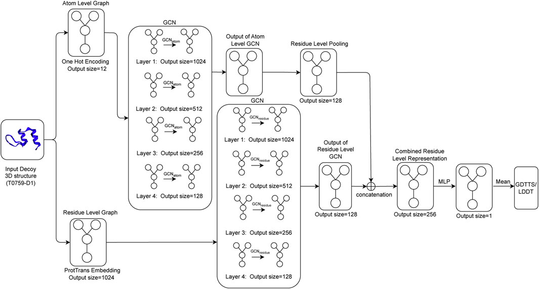
FIGURE 2. Q_ϵ model architecture illustrating how an input decoy structure is propagated through multiple graph convolutional layers (GCN_atom for the atom-level representation and GCN_residue for the residue-level representation of a protein); the outputs of the two sets of convolutional layers are concatenated and fed through a multi-layer perceptron (MLP) to generate local scores that are then averaged to compute the predicted GDTTS or lDDT score.

3.4 Atom and residue features

Our method performs convolution at both the atom and residue levels. Here, we describe the features used at both levels.

3.4.1 Atom features

We represent the atoms using one-hot encoding by grouping atoms into 11 different types (Derevyanko et al., 2018). This grouping reflects both the type of atom (carbon, oxygen, or nitrogen) and its context within the residue (e.g., alpha carbon or the different group an atom belongs to). In doing so, we are able to incorporate important information of the atoms while also capturing the relationships between the atoms and their corresponding residues.

3.4.2 Residue features

We compute residue features by feeding the amino acid sequence of a decoy to the ProtTrans protein language model (Elnaggar et al., 2021). ProtTrans embeddings provide a very useful representation of the amino acid sequence, capturing relationships between residues and their structural context (Elnaggar et al., 2021). We take the embeddings from the last hidden state of the transformer attention stack of the ProtTrans model, with an output embedding of 1,024 dimensions, which serves as the input to the residue-level GCN.

3.5 A modified ϵ-insensitive loss

In this work, we address quality assessment as a regression problem with the objective of predicting GDTTS or lDDT score of a decoy. We propose a novel loss function that captures our desiderata for a quality assessment model: when it comes to poor decoys, we do not care about the accuracy of the prediction as long as we can differentiate it from a good decoy. On the other hand, the more accurate the decoy, the more accurate we want our prediction to be. This is especially important given the recent improvement in the quality of protein structure prediction methods. To achieve this goal, we modify the ϵ-insensitive loss, which is the loss function employed in SVM regression (Drucker et al., 1996), as follows:

$L\left(y,y^{\prime }\right)=\mathit{max}\left(0,|y-y^{\prime }|-ϵ\left(y\right)\right),(3)$

where y and y′ are the true and predicted scores, respectively. As in the standard ϵ-insensitive loss, this defines a tube of size ϵ within which there is no penalty; outside the tube, the loss grows linearly as in the L1-loss, which is defined as L(y, y′) = |y − y′|. In our application, the size of the tube is a function ϵ(y). In this work, we used a tube defined as shown in Figure 3. The motivation for the modified ϵ-insensitive loss function is that the model should not try too hard to accurately fit poor-quality decoys where we do not need good accuracy anyhow. As decoy quality increases, models are trained to learn a fit that is much more accurate.

FIGURE 3

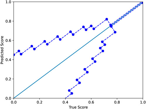
FIGURE 3. The modified ϵ-insensitive loss uses a variable-sized band around the diagonal in which a predicted score is not penalized. The band becomes smaller as the GDTTS or lDDT score increases, reflecting our expectation for precise predictions for decoys that are closer to the native structure.

3.6 Network training

We have trained our network to predict GDTTS and lDDT score. For GDTTS prediction, we first pre-train Q_ϵ with the L1-loss for 50 epochs, followed by training with the modified ϵ-insensitive loss for the next 10 epochs. To train the network with lDDT scores, we select the best model from GDTTS (“best” with respect to the validation set) and train it with the modified ϵ-insensitive loss for another 50 epochs, keeping the same network architecture and hyperparameters.

The network was implemented in PyTorch (Paszke et al., 2019) and optimized using the Adam method (Kingma and Ba, 2014) with default parameters except for a learning rate of 0.001; training used a batch size of 70. Since our training set is highly imbalanced, i.e., contains very few high-quality decoys, we used the imbalanced sampler from the torchsampler package. During training, we monitored the loss over the validation set and used the model that gave the minimum loss. Our implementation used the PyTorch Lightning framework for training and testing and PyTorch Geometric (Fey and Lenssen, 2019) for performing graph convolution. Model selection was performed using the hyperparameters and values described in Table 1. We iterated over all parameters and, for each one, chose the value that gave the highest Pearson correlation coefficient on the validation set. Following model selection, training took approximately 42 h on an NVIDIA RTX 3090 GPU.

TABLE 1

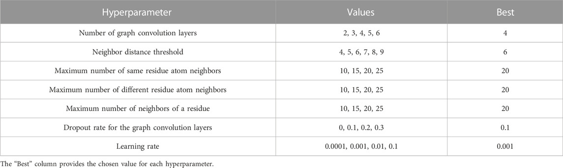
TABLE 1. Hyperparameter space. Model selection was performed based on performance on the validation set.

3.7 Data

We collected decoys from CASP9 to CASP14 along with their labels from the CASP website (CASP, 2021). We used CASP9–CASP12 as our training and validation sets and CASP13 and CASP14 as our test sets (see Table 2). In order to match the decoys used in experiments performed by others, we created two separate datasets for GDDTS evaluation (CASP13 and CASP14) and two datasets for the evaluation of lDDT score prediction (CASP13 and CASP14).

TABLE 2

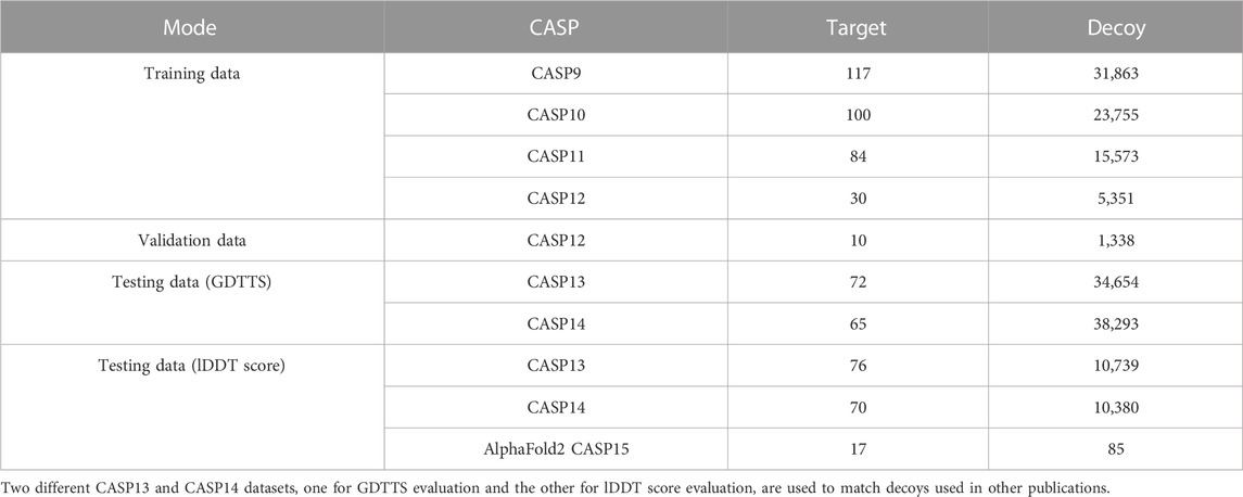
TABLE 2. Number of targets from CASP competitions in the training, validation, and testing data.

In CASP15, the focus shifted from predicting the accuracy of single-chain decoys to that of multi-chain complexes (Kryshtafovych et al., 2023). However, some of the targets were composed of single chains, and we chose to focus on those targets in our evaluation, leading to a dataset with 17 targets.

4 Results

We compare Q_ϵ with other methods that have either state-of-the-art or very good performance in CASP13 and CASP14. In our first set of experiments, we sought to compare our method with GraphQA, which uses a similar graph convolution architecture and was trained to predict GDTTS (Baldassarre et al., 2020). The results in Table 3 indicate that Q_ϵ outperforms GraphQA and several other recent methods trained to predict GDTTS despite not using engineered features; a detailed analysis of the contribution of the various components of the Q_ϵ architecture is described in an ablation study in the following section.

TABLE 3

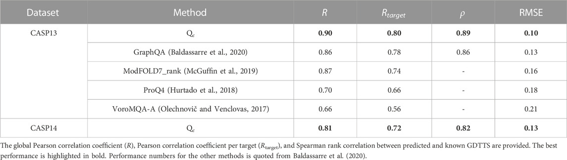
TABLE 3. Performance of Q_ϵ and other methods in CASP13 and CASP14 GDTTS prediction.

The quality assessment community is transitioning to the use of the lDDT score, so we also compare Q_ϵ with more recent methods evaluated with lDDT. In this evaluation, the performance of Q_ϵ was similar to that of DeepUMQA but outperformed by its successor, DeepUMQA2 (see Table 4). Results from EnQA (Chen et al., 2023), whose performance was similar to that of DeepUMQA2, are also better than those of Q_ϵ. Both methods use more complex architectures and extensive engineered features; DeepUMQA2 also used evolutionary information, including structural features from homologous templates.

TABLE 4

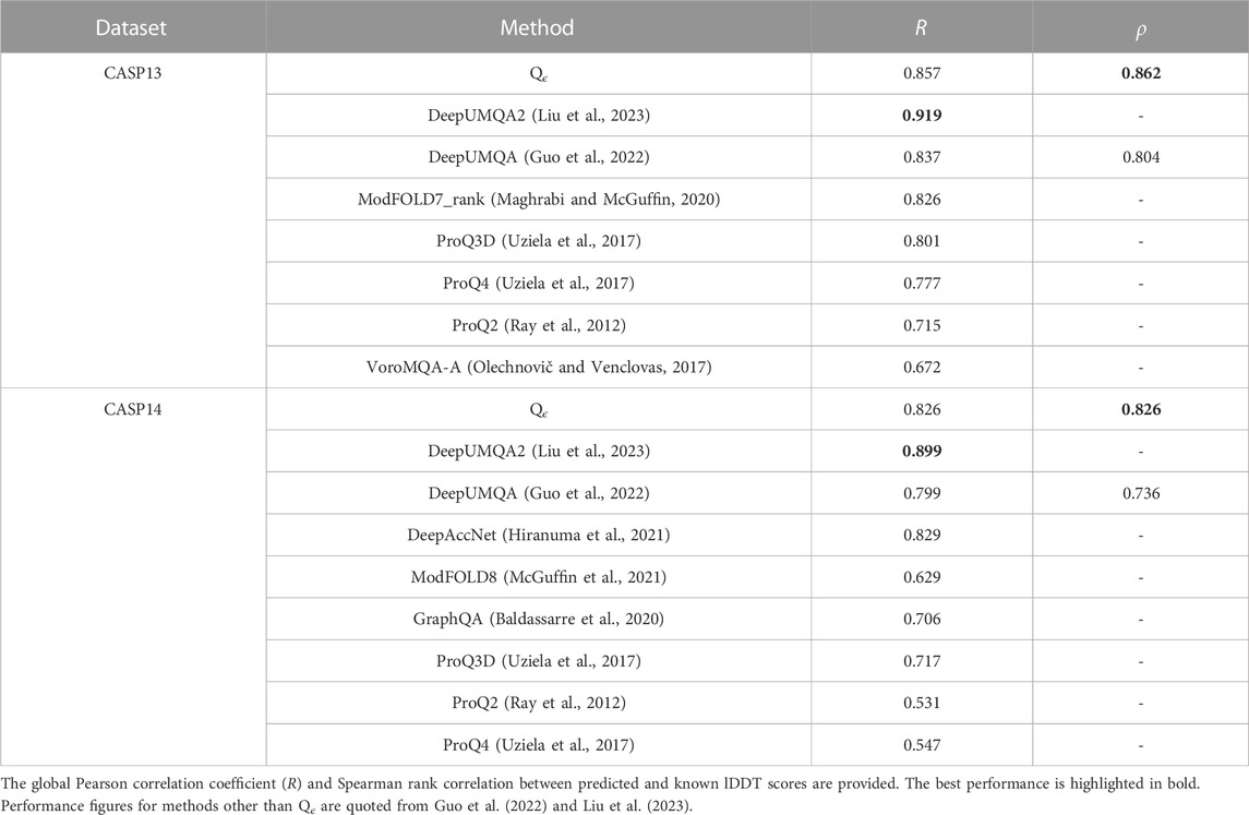
TABLE 4. Performance of Q_ϵ and other methods in CASP13 and CASP14 with respect to lDDT scores.

To understand the contribution of the proposed modified ϵ-insensitive loss to the performance of Q_ϵ, a scatter plot of true versus predicted GDTTS for the decoys in CASP13 and CASP14 is shown in Figure 4. We observe that the modified ϵ-insensitive loss leads to better learning of decoys of all quality levels compared to the L1-loss and leads to a pattern where the predictions are limited to a band around the true scores, which is a highly desirable property for a quality assessment method. It was interesting that the width of the band is similar across all quality levels, despite the loss having a variable width band compared to the original ϵ-insensitive loss function.

FIGURE 4

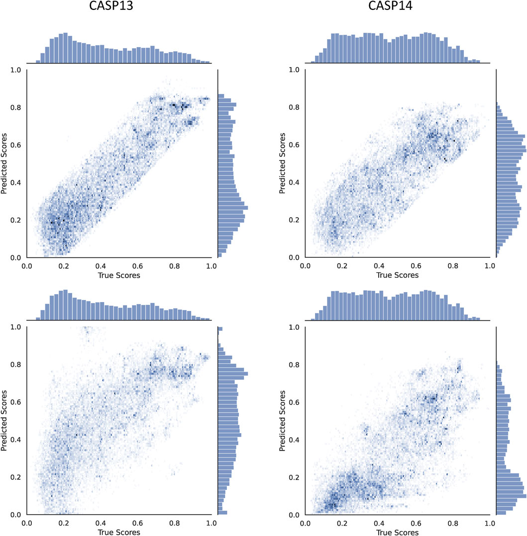
FIGURE 4. Scatter plots comparing the true and predicted GDTTS for both CASP13 and CASP14 using L1-loss (bottom) and modified ε-insensitive loss (top).

4.1 Ablation study

To demonstrate the contribution of each of the major components of our method, we performed an ablation study with respect to GDTTS prediction, and its results are shown in Table 5. The first component we varied was the loss function. We observe that the pre-training with the L1-loss is key for the method’s performance, serving to bootstrap the learning process. We also observe that performance dropped when using the original ϵ-insensitive loss function, L1-loss, or L2-loss. This clearly shows the contribution of the proposed modification to the ϵ-insensitive loss. Our next observation is that both the residue-level and atom-level convolutional blocks are crucial for the performance of the method. This is due to each of them providing different and complementary information. The residue-level blocks use ProtTrans embeddings, which have been documented to provide a variety of information regarding a residue’s evolutionary history and structural context within the protein (Elnaggar et al., 2021). The atom-level convolutional blocks provide a more fine-grained view of a decoy structure, complementing the information at the residue level.

TABLE 5

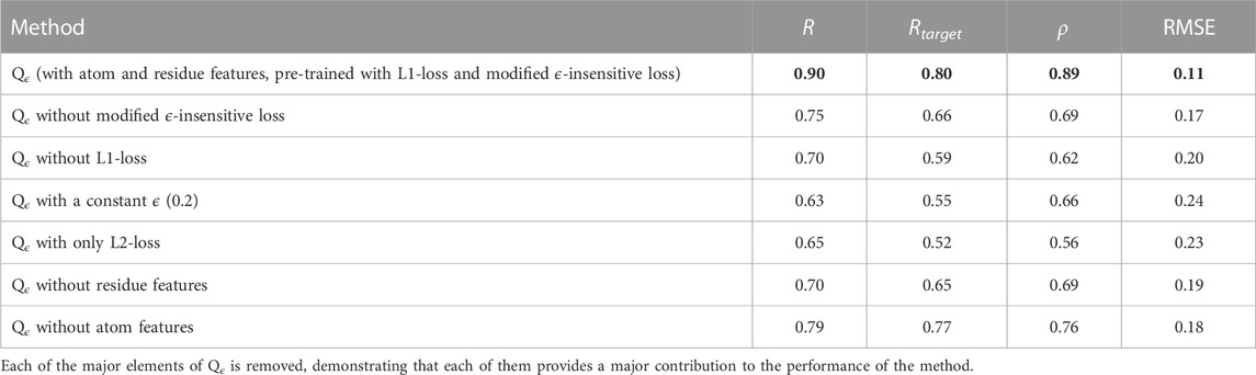
TABLE 5. Q_ϵ ablation study.

4.2 ϵ-threshold selection

The modified ϵ-insensitive loss has nine threshold parameters associated with the epsilon insensitive loss function, one for each bin of the prediction score. In our experiments, we have used the values shown in Figure 3. In order to determine that our initial choice was good, we ran an experiment where we varied all the values in a coordinated manner: we chose nine values lower or higher than the initial values (the columns low and high in Table 6). As shown in Table 6, reducing or increasing the values of all the thresholds in a coordinated fashion led to reduced accuracy on the validation set. As a sanity check, we verified that a similar decrease is observed on the test set as well.

TABLE 6

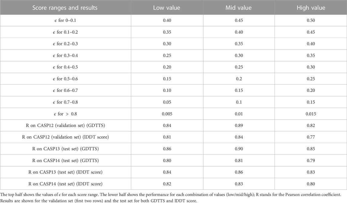
TABLE 6. Model selection over the ϵ hyperparameter values.

4.3 Local quality assessment with Q_ϵ

In this section, we demonstrate the ability of Q_ϵ to make accurate predictions at the residue level, despite being trained only on global quality scores. This ability is a byproduct of the architecture of the network, where the global predicted score is an average of residue-level node summary scores (see Figure 2). This forces the network to learn accurate local scores, as demonstrated in the results shown in Table 7. Similar to the global prediction problem, the performance of Q_ϵ is between that of DeepUMQA and DeepUMQA2.

TABLE 7

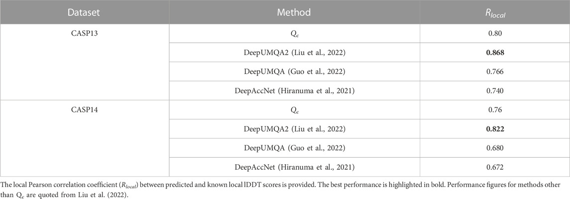
TABLE 7. Performance of Q_ϵ and other methods in CASP13 and CASP14 with respect to local lDDT scores.

4.4 Results on CAMEO decoys

For further validation of the performance of Q_ϵ, we evaluated its performance on decoys from the CAMEO evaluation project (Haas et al., 2018). We downloaded decoys used from 13 May 2022 to 06 May 2023 and followed the same evaluation protocol used by CAMEO: the area under the ROC (AUROC) curve and area under the precision recall (AUPR) curve were calculated using a local lDDT score threshold of 0.6, and the obtained results are shown in Table 8. Again, we note that Q_ϵ was not trained on local scores (unlike the other methods) and yet is able to perform almost on par with DeepUMQA2. As mentioned previously, this can be traced to the fact that the global prediction score computed by Q_ϵ is evaluated by directly averaging local node summary scores, forcing those scores to reflect a local measure of quality.

TABLE 8

TABLE 8. Performance of Q_ϵ and other methods on the CAMEO dataset.

4.5 Performance on AlphaFold2 decoys

In CASP14, AlphaFold2 provided, for the first time, decoys with near experimental resolution (Skolnick et al., 2021), with a median GDTTS of 92.4, making it the first team to achieve the highest level of accuracy in CASP. We gathered the decoys submitted by the AlphaFold team (team no 427) from the CASP14 website and evaluated Q_ϵ on their decoys. We also ran AlphaFold2 version 2.3.1 on CASP15 single-chain targets. The results of this experiment are shown in Table 9. While AlphaFold2 provided better accuracy than our method, its value provided independent validation for the quality of AlphaFold2 predictions. EnQA (Chen et al., 2023) slightly improves on the quality of AlphaFold2 lDDT score estimates; however, it does so by using the AlphaFold2 scores as one of its features. Therefore, the results of the EnQA method are expected to be highly correlated with those of AlphaFold2 and less useful for independent verification of its predictions.

TABLE 9

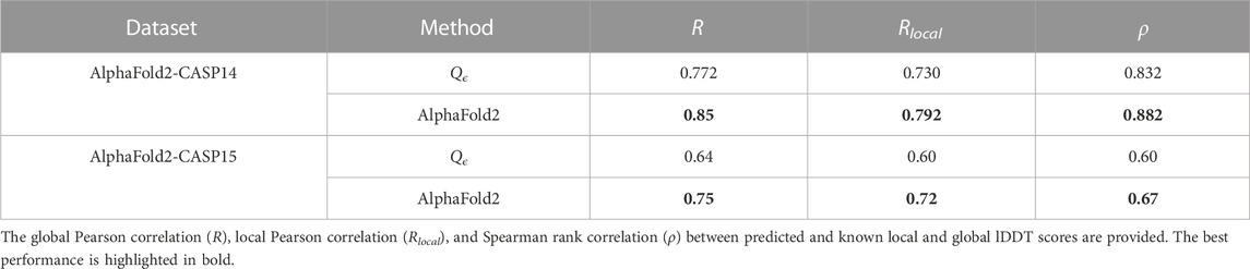
TABLE 9. Performance of Q_ϵ and AlphaFold2 on AlphaFold2-generated decoys in CASP14 and CASP15.

5 Conclusion and future work

In this study, we proposed a novel loss function to enhance the performance of deep learning for quality assessment of decoy structures. Our approach performed close to other state-of-the-art methods while at the same time removing the need for engineered features computed from the protein structure, relying solely on features computed from the decoy sequence, demonstrating what is possible with a pure deep learning approach. These features were integrated using graph convolutional layers that operate at both the atom and residue levels, thereby improving the network’s performance. The comparison of our approach with AlphaFold2 indicates there is a need for further research to provide accuracy estimates that improve on the local scores computed by AlphaFold2 in order to provide independent validation of the quality of its predicted structures.

Our approach can be extended in multiple ways. First, although it performs well in predicting local scores, the method is trained using only global quality scores. Joint learning of both global and local scores can potentially improve performance for both tasks. Second, we treated the prediction of GDDTS and lDDT score as independent tasks; there is a potential gain in addressing multiple quality scores at the same time (Baldassarre et al., 2020). Finally, in this work, we chose to focus on the contribution of the loss function to method performance, so we used a relatively simple graph convolutional network similar to that used in GraphQA (Baldassarre et al., 2020). Finally, we expect that the proposed loss function can be applied to regression problems, whose objective is to detect high-quality objects, and has the potential to be a useful addition to any deep learning toolbox.

Data availability statement

The datasets presented in this study can be found in online repositories. The names of the repository/repositories and accession number(s) can be found in the article/Supplementary Material.

Author contributions

This study was conceived by AB-H, and all the experiments were performed by SR. SR and AB-H analyzed the results and wrote the manuscript. All authors contributed to the article and approved the submitted version.

Funding

This project was supported by NSF-ABI award #1564840.

Acknowledgments

The authors would like to thank Jianlin Cheng for fruitful discussions on the quality assessment problem.

Conflict of interest

The authors declare that the research was conducted in the absence of any commercial or financial relationships that could be construed as a potential conflict of interest.

Publisher’s note

All claims expressed in this article are solely those of the authors and do not necessarily represent those of their affiliated organizations, or those of the publisher, the editors, and the reviewers. Any product that may be evaluated in this article, or claim that may be made by its manufacturer, is not guaranteed or endorsed by the publisher.

References

Akhter, N., Chennupati, G., Djidjev, H., and Shehu, A. (2020). Decoy selection for protein structure prediction via extreme gradient boosting and ranking. BMC Bioinformatics 21, 189. doi:10.1186/s12859-020-3523-9

PubMed Abstract | CrossRef Full Text | Google Scholar

Al-Lazikani, B., Jung, J., Xiang, Z., and Honig, B. (2001). Protein structure prediction. Curr. Opin. Chem. Biol. 5, 51–56. doi:10.1016/s1367-5931(00)00164-2

PubMed Abstract | CrossRef Full Text | Google Scholar

Baldassarre, F., Menéndez Hurtado, D., Elofsson, A., and Azizpour, H. (2020). GraphQA: protein model quality assessment using graph convolutional networks. Bioinformatics 37, 360–366. doi:10.1093/bioinformatics/btaa714

CrossRef Full Text | Google Scholar

CASP (2021). CASP. [Dataset]. Available at: https://predictioncenter.org/download_area/.

Google Scholar

Chen, C., Chen, X., Morehead, A., Wu, T., and Cheng, J. (2023). 3D-equivariant graph neural networks for protein model quality assessment. Bioinformatics 39, btad030. doi:10.1093/bioinformatics/btad030

PubMed Abstract | CrossRef Full Text | Google Scholar

Cheng, J., Choe, M.-H., Elofsson, A., Han, K.-S., Hou, J., Maghrabi, A. H., et al. (2019). Estimation of model accuracy in CASP13. Proteins Struct. Funct. Bioinforma. 87, 1361–1377. doi:10.1002/prot.25767

PubMed Abstract | CrossRef Full Text | Google Scholar

Derevyanko, G., Grudinin, S., Bengio, Y., and Lamoureux, G. (2018). Deep convolutional networks for quality assessment of protein folds. Bioinformatics 34, 4046–4053. doi:10.1093/bioinformatics/bty494

PubMed Abstract | CrossRef Full Text | Google Scholar

Drucker, H., Burges, C. J. C., Kaufman, L., Smola, A., and Vapnik, V. (1996). “Support vector regression machines,” in Advances in neural information processing systems. Editors M. Mozer, M. Jordan, and T. Petsche (MIT Press), 9, 155–161.

Google Scholar

Elnaggar, A., Heinzinger, M., Dallago, C., Rehawi, G., Wang, Y., Jones, L., et al. (2021). ProtTrans: toward understanding the language of life through self-supervised learning. IEEE Trans. pattern analysis Mach. Intell. 44, 7112–7127. doi:10.1109/tpami.2021.3095381

CrossRef Full Text | Google Scholar

Fey, M., and Lenssen, J. E. (2019). Fast graph representation learning with PyTorch Geometric. arXiv preprint arXiv:1903.02428.

Google Scholar

Fout, A., Byrd, J., Shariat, B., and Ben-Hur, A. (2017). Protein interface prediction using graph convolutional networks, 30.

Google Scholar

Guo, S.-S., Liu, J., Zhou, X.-G., and Zhang, G.-J. (2022). DeepUMQA: ultrafast shape recognition-based protein model quality assessment using deep learning. Bioinformatics 38, 1895–1903. doi:10.1093/bioinformatics/btac056

PubMed Abstract | CrossRef Full Text | Google Scholar

Haas, J., Barbato, A., Behringer, D., Studer, G., Roth, S., Bertoni, M., et al. (2018). Continuous Automated Model EvaluatiOn (CAMEO) complementing the critical assessment of structure prediction in CASP12. Proteins Struct. Funct. Bioinforma. 86, 387–398. doi:10.1002/prot.25431

PubMed Abstract | CrossRef Full Text | Google Scholar

Hiranuma, N., Park, H., Baek, M., Anishchenko, I., Dauparas, J., and Baker, D. (2021). Improved protein structure refinement guided by deep learning based accuracy estimation. Nat. Commun. 12, 1340. doi:10.1038/s41467-021-21511-x

PubMed Abstract | CrossRef Full Text | Google Scholar

Hurtado, D. M., Uziela, K., and Elofsson, A. (2018). Deep transfer learning in the assessment of the quality of protein models. arXiv preprint arXiv:1804.06281.

Google Scholar

Ioffe, S., and Szegedy, C. (2015). “Batch normalization: accelerating deep network training by reducing internal covariate shift,” in International conference on machine learning (pmlr), 448–456.

Google Scholar

Jumper, J., Evans, R., Pritzel, A., Green, T., Figurnov, M., Ronneberger, O., et al. (2021). Highly accurate protein structure prediction with alphafold. Nature 596, 583–589. doi:10.1038/s41586-021-03819-2

PubMed Abstract | CrossRef Full Text | Google Scholar

Kingma, D. P., and Ba, J. (2014). Adam: A method for stochastic optimization. arXiv preprint arXiv:1412.6980

Google Scholar

Kryshtafovych, A., Antczak, M., Szachniuk, M., Zok, T., Kretsch, R. C., Rangan, R., et al. (2023). New prediction categories in casp15. Proteins Struct. Funct. Bioinforma. doi:10.1002/prot.26515

CrossRef Full Text | Google Scholar

Liu, J., Zhao, K., and Zhang, G. (2022). Improved model quality assessment using sequence and structural information by enhanced deep neural networks. Briefings Bioinforma. 24, bbac507. doi:10.1093/bib/bbac507

CrossRef Full Text | Google Scholar

Liu, J., Zhao, K., and Zhang, G. (2023). Improved model quality assessment using sequence and structural information by enhanced deep neural networks. Briefings Bioinforma. 24, bbac507. doi:10.1093/bib/bbac507

CrossRef Full Text | Google Scholar

Lundström, J., Rychlewski, L., Bujnicki, J., and Elofsson, A. (2001). Pcons: A neural-network–based consensus predictor that improves fold recognition. Protein Sci. 10, 2354–2362. doi:10.1110/ps.08501

PubMed Abstract | CrossRef Full Text | Google Scholar

Maghrabi, A. H., and McGuffin, L. J. (2020). Estimating the quality of 3D protein models using the ModFOLD7 server. Protein Struct. Predict. 2165, 69–81. doi:10.1007/978-1-0716-0708-4_4

PubMed Abstract | CrossRef Full Text | Google Scholar

Mariani, V., Biasini, M., Barbato, A., and Schwede, T. (2013). lDDT: a local superposition-free score for comparing protein structures and models using distance difference tests. Bioinformatics 29, 2722–2728. doi:10.1093/bioinformatics/btt473

PubMed Abstract | CrossRef Full Text | Google Scholar

McGuffin, L. J., Adiyaman, R., Maghrabi, A. H., Shuid, A. N., Brackenridge, D. A., Nealon, J. O., et al. (2019). IntFOLD: an integrated web resource for high performance protein structure and function prediction. Nucleic acids Res. 47, W408–W413. doi:10.1093/nar/gkz322

PubMed Abstract | CrossRef Full Text | Google Scholar

McGuffin, L. J., Aldowsari, F. M., Alharbi, S. M., and Adiyaman, R. (2021). ModFOLD8: accurate global and local quality estimates for 3D protein models. Nucleic acids Res. 49, W425–W430. doi:10.1093/nar/gkab321

PubMed Abstract | CrossRef Full Text | Google Scholar

McGuffin, L. J., Edmunds, N. S., Genc, A. G., Alharbi, S. M., Salehe, B. R., and Adiyaman, R. (2023). Prediction of protein structures, functions and interactions using the IntFOLD7, MultiFOLD and ModFOLDdock servers. Nucleic Acids Res., gkad297. doi:10.1093/nar/gkad297

PubMed Abstract | CrossRef Full Text | Google Scholar

Moult, J., Pedersen, J. T., Judson, R., and Fidelis, K. (1995). A large-scale experiment to assess protein structure prediction methods. Proteins. [Dataset]. doi:10.1002/prot.340230303

CrossRef Full Text | Google Scholar

Olechnovič, K., and Venclovas, Č. (2017). VoroMQA: assessment of protein structure quality using interatomic contact areas. Proteins Struct. Funct. Bioinforma. 85, 1131–1145. doi:10.1002/prot.25278

CrossRef Full Text | Google Scholar

Pagès, G., Charmettant, B., and Grudinin, S. (2019). Protein model quality assessment using 3D oriented convolutional neural networks. Bioinformatics 35, 3313–3319. doi:10.1093/bioinformatics/btz122

PubMed Abstract | CrossRef Full Text | Google Scholar

Paszke, A., Gross, S., Massa, F., Lerer, A., Bradbury, J., Chanan, G., et al. (2019). PyTorch: an imperative style, high-performance deep learning library. Adv. neural Inf. Process. Syst. 32.

Google Scholar

Ray, A., Lindahl, E., and Wallner, B. (2012). Improved model quality assessment using ProQ2. BMC Bioinforma. 13, (224). doi:10.1186/1471-2105-13-224

PubMed Abstract | CrossRef Full Text | Google Scholar

Shehu, A. (2015). A review of evolutionary algorithms for computing functional conformations of protein molecules. Computer-Aided Drug Discov., 31–64. doi:10.1007/7653_2015_47

CrossRef Full Text | Google Scholar

Skolnick, J., Gao, M., Zhou, H., and Singh, S. (2021). AlphaFold 2: why it works and its implications for understanding the relationships of protein sequence, structure, and function. J. Chem. Inf. Model. 61, 4827–4831. doi:10.1021/acs.jcim.1c01114

PubMed Abstract | CrossRef Full Text | Google Scholar

Uziela, K., Shu, N., Wallner, B., and Elofsson, A. (2016). ProQ3: improved model quality assessments using Rosetta energy terms. Sci. Rep. 6, 33509–33510. doi:10.1038/srep33509

PubMed Abstract | CrossRef Full Text | Google Scholar

Uziela, K., Menendez Hurtado, D., Shu, N., Wallner, B., and Elofsson, A. (2017). ProQ3D: improved model quality assessments using deep learning. Bioinformatics 33, 1578–1580. doi:10.1093/bioinformatics/btw819

PubMed Abstract | CrossRef Full Text | Google Scholar

Varadi, M., Anyango, S., Deshpande, M., Nair, S., Natassia, C., Yordanova, G., et al. (2022). AlphaFold protein structure database: massively expanding the structural coverage of protein-sequence space with high-accuracy models. Nucleic acids Res. 50, D439–D444. doi:10.1093/nar/gkab1061

PubMed Abstract | CrossRef Full Text | Google Scholar

Wallner, B., and Elofsson, A. (2003). Can correct protein models be identified? Protein Sci. 12, 1073–1086. doi:10.1110/ps.0236803

PubMed Abstract | CrossRef Full Text | Google Scholar

Zemla, A. (2003). LGA: a method for finding 3D similarities in protein structures. Nucleic Acids Res. 31, 3370–3374. doi:10.1093/nar/gkg571

PubMed Abstract | CrossRef Full Text | Google Scholar