 Daniel J. Burt
 Friederike Fröb
 Tatiana Ilyina
- 1Max Planck Institute for Meteorology, The Ocean in the Earth System, Max Planck Society, Hamburg, Germany
- 2International Max Planck Research School on Earth System Modelling, Max Planck Society, Hamburg, Germany
Ocean Alkalinity Enhancement (OAE) simultaneously mitigates atmospheric concentrations of CO2 and ocean acidification; however, no previous studies have investigated the response of the non-linear marine carbonate system sensitivity to alkalinity enhancement on regional scales. We hypothesise that regional implementations of OAE can sequester more atmospheric CO2 than a global implementation. To address this, we investigate physical regimes and alkalinity sensitivity as drivers of the carbon-uptake potential response to global and different regional simulations of OAE. In this idealised ocean-only set-up, total alkalinity is enhanced at a rate of 0.25 Pmol a-1 in 75-year simulations using the Max Planck Institute Ocean Model coupled to the HAMburg Ocean Carbon Cycle model with pre-industrial atmospheric forcing. Alkalinity is enhanced globally and in eight regions: the Subpolar and Subtropical Atlantic and Pacific gyres, the Indian Ocean and the Southern Ocean. This study reveals that regional alkalinity enhancement has the capacity to exceed carbon uptake by global OAE. We find that 82–175 Pg more carbon is sequestered into the ocean when alkalinity is enhanced regionally and 156 PgC when enhanced globally, compared with the background-state. The Southern Ocean application is most efficient, sequestering 12% more carbon than the Global experiment despite OAE being applied across a surface area 40 times smaller. For the first time, we find that different carbon-uptake potentials are driven by the surface pattern of total alkalinity redistributed by physical regimes across areas of different carbon-uptake efficiencies. We also show that, while the marine carbonate system becomes less sensitive to alkalinity enhancement in all experiments globally, regional responses to enhanced alkalinity vary depending upon the background concentrations of dissolved inorganic carbon and total alkalinity. Furthermore, the Subpolar North Atlantic displays a previously unexpected alkalinity sensitivity increase in response to high total alkalinity concentrations.
1. Introduction
Ocean Alkalinity Enhancement (OAE) is a strategy to remove CO2 directly from the atmosphere by adding processed minerals [e.g., lime (Ca(OH)2) or olivine (Mg2SiO4)] to marine areas. OAE increases the CO2 buffering capacity of the ocean (de Coninck et al., 2018), which subsequently strengthens the oceanic CO2 uptake (Köhler et al., 2010; Hartmann et al., 2013). The addition of processed minerals is an acceleration of the natural delivery of weathered material that currently leads to the sequestration of ~0.25 PgC a-1 (Taylor et al., 2016). Previous simulations of global alkalinity enhancement reveal spatially heterogeneous changes in the oceanic carbon inventories (Keller et al., 2014; González and Ilyina, 2016; Fröb et al., 2020), which indicates a regional sensitivity to alkalinity enhancement. Here, we investigate the drivers of these regional sensitivities and the response of the non-linear marine carbonate system to OAE.
The oceanic CO2 uptake is strengthened by OAE because of the non-linearity of the marine carbonate system, which modulates the transfer of CO2 between the atmosphere and ocean. Total Alkalinity (TA), defined as the weighted sum of charged ion concentrations in seawater (Dickson, 1981; Zeebe and Wolf-Gladrow, 2003), is added by dissolving alkaline minerals, which release proton acceptors that bind with free hydrogen ions and increase pH (Renforth and Henderson, 2017; Middelburg et al., 2020). The decreased hydrogen ion concentration shifts the dissolution equilibrium of CO2, favouring the dissociation of aqueous CO2 to bicarbonate (HCO3−) ions (Zeebe and Wolf-Gladrow, 2003; Renforth and Henderson, 2017). The establishment of this new balance of the carbonate system in seawater reduces the concentration of aqueous CO2. Subsequently the partial pressure relative to the atmosphere decreases, which leads to a higher CO2 solubility. While the dissociation equilibrium is dependent upon the partial pressure of CO2, temperature and salinity (Renforth and Henderson, 2017; Middelburg et al., 2020), the magnitude of the enhanced CO2 sequestration due to OAE depends on the initial state of the marine carbonate system (Köhler et al., 2010).
González and Ilyina (2016) propose that physical regimes, which influence temperature and salinity, and marine carbonate system states drive the regionally varying response to global OAE in their simulations. However, previous simulations of regionally deployed alkalinity enhancement reach seemingly contradictory conclusions. In a pioneering study to assess the potential of alkalinity enhancement to mitigate atmospheric CO2 and ocean acidification, Ilyina et al. (2013b) conclude that the carbon-uptake potential of an OAE pulse depends on the dominant hydrodynamic regime. In contrast, a later study by Lenton et al. (2018) to determine CO2 sequestration under different emission scenarios finds little sensitivity in the global response to OAE applied across different latitudinal bands. The comparability of these studies is limited primarily by their experimental designs, unlimited (Ilyina et al., 2013b) in contrast to limited (Lenton et al., 2018) alkalinity enhancement, and the use of models of varying complexity, ocean-only (Ilyina et al., 2013b) vs. Earth system (Lenton et al., 2018). As of now, it is still unknown what influence physical circulation and marine carbonate system states have on regional alkalinity enhancement and, subsequently, on the CO2 buffering capacity and alkalinity sensitivity.
We evaluate the influence of physical circulation and marine carbonate system states on alkalinity enhancement in simulations of global and regional OAE using an idealised set-up of the ocean-only model, MPIOM-HAMOCC. To investigate the impact of OAE on the CO2 buffering capacity, we quantify the impact of alkalinity enhancement globally and across eight selected regions on oceanic CO2 sequestration. Furthermore, we analyse the response of alkalinity sensitivity with simulated deployments of global and regional OAE.
2. Methodology
2.1. Model Description
Our experiments are simulated using the physical and biogeochemical ocean model components of the Max Planck Institute for Meteorology Earth System Model version 1.2 (MPI-ESM1.2) as used in the 6th-phase of the Coupled Model Intercomparison Project (Mauritsen et al., 2019). The Max Planck Institute Ocean Model version 1.6 (MPIOM1.6) simulates the physical ocean and the oceanic components of the cryosphere (Marsland et al., 2003; Jungclaus et al., 2013; Mauritsen et al., 2019) and provides the 3-dimensional flow fields and turbulent mixing schemes required for the advection and mixing of biogeochemical tracers (Ilyina et al., 2013a; Mauritsen et al., 2019). The HAMburg Ocean Carbon Cycle version 6 (HAMOCC6) model simulates the transport and evolution of biogeochemical tracers at the air-sea interface and within the water column and surface sediment layers of the global ocean (Ilyina et al., 2013a).
The transport and evolution of biogeochemical tracers simulated by HAMOCC6 provides a limited representation of the ocean biogeochemistry response to OAE. Within HAMOCC6, the organic compartments are resolved through an extended Nutrient, Phytoplankton, Zooplankton and Detritus scheme (Six and Maier-Reimer, 1996) with prognostic parameterisations of bulk phytoplankton, cyanobacteria and zooplankton (Ilyina et al., 2013a; Paulsen et al., 2017). Inorganic carbon chemistry within the water column is resolved by HAMOCC6 through two prognostic tracers: Dissolved Inorganic Carbon (DIC) and TA (Ilyina et al., 2013a). DIC is computed as the sum of aqueous CO2, carbonic acid (H2CO3), bicarbonate ions (HCO3−) and carbonate ions (CO32−) (Orr et al., 2017):
Following Orr et al. (2017), TA explicitly considers contributions from carbonate, borate, sulphate, silicate, phosphate, fluoride and water and implicitly considers the influences of ammonia and sulphide:
The solubility dependent uptake of atmospheric CO2 increases DIC without changing TA. Biogeochemical processes such as organic matter production or remineralisation and calcium carbonate (CaCO3) precipitation or dissolution influence both DIC and TA. Seawater TA is further modified by the external input of weathering fluxes, seawater-sediment interactions and changes in the physical seawater properties (Ilyina et al., 2013a).
2.2. Alkalinity Input Subroutine
The alkalinity input subroutine of González and Ilyina (2016) is modified for this study to implement a volumetric weighting scheme of the surface grid cells to account for variable layer thickness and different input areas. The default subroutine increases the prognostic TA tracer in the surface layer of the ocean as a product of an alkalinity correction ratio (González and Ilyina, 2016; González et al., 2018; Sonntag et al., 2018; Fröb et al., 2020). We define the alkalinity input region using a two-dimensional binary mask. The sum volume (Vsum(k, j, i)) of the cells within the masked regions (mask(j, i)) are computed from the layer thickness (D(k, j, i)) and cell area (A(k, j, i)), where the indices represent the vertical (k) and horizontal grid dimensions (j, i). In these experiments, TA is added only to the surface layer (k = 1):
A spatially homogeneous input concentration of the TA tracer (ΔTA) is then determined at each time-step as the quotient of a TA input rate (δ TA) to the sum of the surface layer volume:
The input concentrations must be computed at each time-step to consider the variable surface layer volume produced by the free-surface implementation of the ocean primitive equations (Marsland et al., 2003). The input concentration is then added to the TA tracer computed by HAMOCC6.
2.3. Experimental Design
The coupled-ocean model is used in a standard MPIOM1.6 low-resolution grid configuration (GR1.5) (Jungclaus et al., 2013) and boundary conditions are prescribed using forcing datasets (Röske, 2005; Poli et al., 2016). The GR1.5 configuration is a rotated orthogonal curvilinear grid with a nominal horizontal resolution of 1.5o and 40 vertical levels arranged such that the first 20 levels are within the upper 700 m of the ocean (Jungclaus et al., 2013). The system is forced at each 30 min time-step by surface boundary conditions based on the European Centre for Medium-range Weather Forecasts (ECMWF) ERA-20C re-analysis dataset (Poli et al., 2016) with a reduced temporal resolution from 4- to 8-h. The forcing data is applied repetitively with a periodicity of 25 years using the years 1905–1930 as used to reproduce a pre-industrial ocean state in previous studies (DeVries et al., 2019; Liu et al., 2021). These data are combined with continental runoff forcing data for the Ocean Model Intercomparison Project (Röske, 2005).
Biological parameters in HAMOCC6 require tuning to account for grid resolution features and coupling or forcing frequencies (Mauritsen et al., 2019). Coupling or forcing frequencies which resolve diurnal variations in incoming solar radiation can produce a strong depletion of primary producer standing stocks due to high night-time mortality of primary producers in the model. The variables tuned in order to maintain the nitrogen and carbon source-sink dynamics under these conditions are: the maximum growth and mortality rates of cyanobacteria and the grazing rate on bulk phytoplankton (Paulsen et al., 2017). The maximum growth rate of cyanobacteria is increased from 0.2 to 0.3 d-1, the cyanobacteria mortality rate is reduced from 0.1 d-1 to 0.07 d-1 and the grazing rate on bulk phytoplankton is reduced from 1 d-1 to 0.7 d-1. This tuning produces a lower mean N2 fixation rate (~68 Tg N a-1) than the 82 Tg N a-1 which is reported for the MPI-ESM1.2-LR configuration (Mauritsen et al., 2019), and is lower than the range of observation-based estimates of 70–200 Tg N a-1 (Karl et al., 2002; Großkopf et al., 2012). The resulting carbon export (~7.1 Gt C a-1) is greater than the 6.7 Gt C a-1 simulated in the MPI-ESM1.2-LR (Mauritsen et al., 2019) but within the reported range of export fluxes (3-20 Gt C a-1) (Najjar et al., 2007).
Ocean-only experiments are simulated over 75 years for a pre-industrial control and for global and eight regional OAE deployments (section 2.4) each with a fixed atmospheric CO2 mixing ratio of 280 ppm. The simulations are initialised from a quasi-stable model state, which has been spun-up under prescribed pre-industrial forcing (Röske, 2005; Poli et al., 2016); the initial condition is taken 600 years after the last change made during the model spin-up. This idealised set-up permits the investigation of short-term impacts on the marine carbonate system as a result of OAE for the mitigation of the atmospheric CO2 mixing ratio. For comparability, the rate of alkalinity enhancement described by Lenton et al. (2018) is implemented; δTA = 0.25Pmola−1. While the surface areas of the defined global and eight regions are constant throughout the experiments, variations of surface wind speeds over time in the atmospheric forcing produce fluctuations of sea surface height, which lead to temporally varying volumes in the defined surface layer. The input concentration relative to the constant rate of alkalinity enhancement is modulated to account for these volume variations. The surface area and spatiotemporal mean input concentration deployed are presented in Table 1.
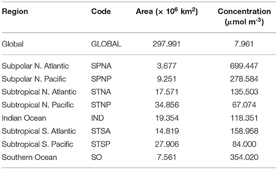
Table 1. Alkalinity enhancement input regions as illustrated in Figure 1, region name abbreviation (code), region surface area and mean concentration of the alkalinity input over the simulation period.
2.4. Definition of Regions
To evaluate the efficiency of regional OAE, eight regions are defined based on a subset of physical conditions in order to represent different hydrographic regimes in the global ocean. It should be noted that regions are not selected with consideration to real-world implementation. The eight selected regions are oriented with respect to persistent, large-scale gyre systems: the Subpolar and the Subtropical Atlantic and Pacific gyres; as well as the Indian Ocean and the Southern Ocean (Figure 1). We identify regions using the climatological (25-year) means of sea surface temperature (SST), salinity (SSS), elevation with respect to the geoid (SSH), the zonal and meridional velocity components, and the horizontal velocity vector from the pre-industrial control of the ocean-only MPIOM simulation. Subpolar and subtropical gyres rotate in opposing directions, producing variations in SSH due to Ekman transport, which can be used to indicate the boundaries between adjacent gyres (Knauss, 2005). We focus only on the open ocean and, therefore, exclude regions with a climatological maximum sea-ice concentration greater than 50% or areas shallower than 200 m.
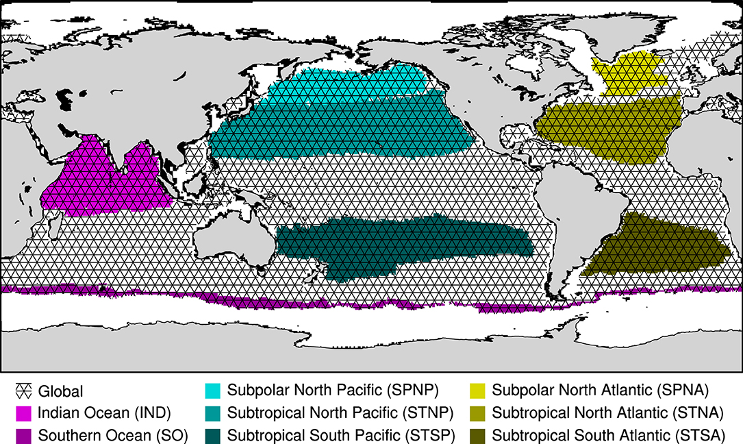
Figure 1. Map of the selected regions: Subpolar North Atlantic - SPNA (light yellow); Subtropical North Atlantic - STNA (yellow); Subtropical South Atlantic - STSA (dark yellow); Subpolar North Pacific - SPNP (light cyan), Subtropical North Pacific - STNP (cyan); Subtropical South Pacific - STSP (dark cyan); Indian Ocean - IND (magenta); Southern Ocean - SO (dark magenta). The Global alkalinity enhancement region (GLOBAL) is indicated by the triangular mesh overlay. Only ice-free, open-ocean areas are included in the global and different regional definitions.
We divide the Atlantic Ocean into three regions associated with major wind-driven gyres. A SSH anomaly of –0.7 m is used to indicate the division between the Subpolar North Atlantic (SPNA) and the Subtropical regions. The Subtropical North Atlantic (STNA) region is constrained with SSSs >35.8. The Subtropical South Atlantic (STSA) region is bound by the strong eastward South Atlantic and northwestward Benguela Current systems. A region of weaker currents, with horizontal velocity vector magnitudes <0.12 m s-1, exists between these boundary currents and the South American continental landmass.
The Southern Ocean (SO) region is bound to the north by the Antarctic Polar Front, which is defined by a horizontal SST gradient of 0.01 K km-1 (Dong et al., 2006). This does not produce a contiguous boundary in the model SST climatological mean. Areas of 0.01 K km-1 occur along a contiguous 4oC SST isotherm, which is substituted for the northern regional boundary.
As with the Atlantic, we separate the Pacific Ocean into three regions associated with major wind-driven gyres. We use the subtropical front between the Pacific Ocean and the Southern Ocean (SSS >34.6) as described by Chaigneau and Pizarro (2005) to define the southern extent of the Subtropical South Pacific (STSP) region. The Indo-Pacific Warm Pool as described by Wyrtki (1989) is not considered representative of the Subtropical South Pacific gyre, therefore SST >28oC are excluded. Zonal (>-0.08 m s-1) and meridional (>-0.09 m s-1) velocity conditions are used to further constrain the STSP region. We define the Subtropical North Pacific (STNP) region with SSH >0.75 m as this provides a strong distinction in the western Pacific from tropical latitudes. In the eastern Pacific, we use SSTs of 12–25oC to define a sector which agrees with the latitudinal extent of the STNP SSH region and continues to the North American continental landmass as an eastern boundary. We characterise the Subpolar North Pacific (SPNP) region with a SSH threshold of <0.075 m. The Sea of Japan, South China Sea and Sea of Okhotsk are not included in the North Pacific regions as they are not representative of the open ocean.
The evaluation of climatological means precludes the evaluation of parameters characterised by the strong seasonal monsoon-cycle in the Northern Indian Ocean (Shetye et al., 1991; Schott et al., 2009; Vinayachandran et al., 2013). Therefore, the Indian Ocean (IND) region is defined as the region north of the strong, prevailing South Equatorial Current in the Indian Ocean where the Red Sea, Gulf of Aden and Gulf of Oman are excluded.
2.5. Model Evaluation
We qualitatively evaluate the 75-year mean states of TA, DIC (Figure 2) and alkalinity sensitivity (Figure 3) from the control experiment against mapped climatologies (Lauvset et al., 2016) based on the Global Ocean Data Analysis Project version 2 data product (GLODAPv2; Olsen et al., 2016). Due to differences in vertical resolution, the surface layer of the model (0–12 m) is compared to the vertical-mean of the topmost two layers (0 m, 10 m) of the mapped climatologies. Unit conversions are performed on model TA and DIC data using local seawater density approximations derived from surface potential temperature and practical salinity data using the Gibbs Seawater Oceanographic Toolbox (TEOS-10; McDougall and Barker, 2011). We evaluate the surface distributions of TA and DIC in the model (Figure 2E) as the magnitude of the carbon-uptake response to OAE is dependent on the background state of the simulated marine carbonate system (Köhler et al., 2010).
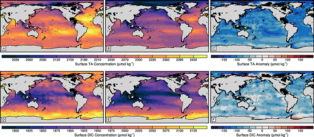
Figure 2. Maps of total alkalinity (A–C) and dissolved inorganic carbon (D–F) of the (A,D) GLODAPv2 mapped climatology (Lauvset et al., 2016) surface vertical-mean, (B,E) 75-year mean surface model control state and (C,F) surface anomalies between the model control and the GLODAPv2 datasets.
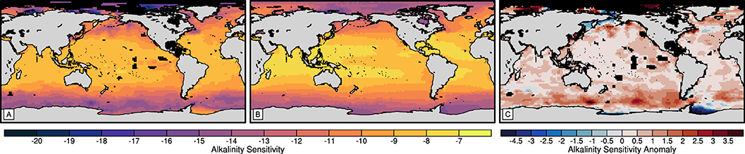
Figure 3. Maps of alkalinity sensitivity derived from the (A) GLODAPv2 climatology surface vertical-mean and (B) 75-year mean surface model control state and (C) alkalinity sensitivity anomalies between the alkalinity sensitivities derived from the model control and GLODAPv2 datasets.
We find that the large-scale pattern of observed surface TA is well reproduced by the model (Figures 2A,B). However, TA is consistently underestimated in the pre-industrial control simulation, with a global annual mean of 2196±97 μmol kg-1, compared to the mapped present-day surface climatology with a global mean of 2297±72 μmol kg-1. The TA anomalies are heterogeneously distributed but uniformly negative across the global ocean (Figure 2C). The underestimation is the result of model tuning toward a net global CO2 flux of 0 GtC a-1 between the ocean and atmosphere. However, the order of magnitude of TA anomalies in our experiments has been found acceptable in previous model studies (Keller et al., 2012; Ilyina et al., 2013a; Matear and Lenton, 2014). Note that the difference between present-day and pre-industrial surface TA is assumed to be minor (Sarmiento and Gruber, 2006; Middelburg et al., 2020). Typically, TA covaries with salinity (Middelburg et al., 2020), and the control (Figure 2B) successfully captures the pattern of high TA at subtropical latitudes, lower TA in equatorial, subpolar and polar regions and generally higher TA in the Atlantic than at similar latitudes in the Pacific. Larger positive and negative anomalies (Figure 2C) are displayed in regions associated with strong circulation regimes, marginal coastal and shelf sea regions and regions associated with strong freshwater fluxes, such as where the Arctic Ocean is influenced by Siberian river systems.
The model control (Figure 2E) also captures the large-scale distribution of surface DIC concentrations, while consistently underestimating the concentrations compared to the GLODAPv2 pre-industrial climatology (Figure 2D). The global mean surface DIC concentration of the model control is 1904±99 μmol kg-1, in contrast to that of the mapped pre-industrial climatology, which is 1966±84 μmol kg-1. The dominant drivers of the latitudinal surface DIC distribution of the GLODAPv2 climatology are temperature and vertical circulation regimes (Wu et al., 2019). The control simulation also exhibits a pattern of surface DIC with the highest concentrations in the Southern Ocean and the lowest concentrations in the coastal equatorial Pacific and eastern Indian Ocean (Figure 2E). The Arctic Ocean and Southern Ocean feature the largest anomalies. While the Arctic Ocean anomalies appear related to the surface TA anomalies, the surface DIC anomalies in the Southern Ocean may indicate poorly resolved vertical circulation in the Weddell Sea. However, the heterogeneity of the anomalies in the open ocean regions pertinent to this study (Figure 2F) indicate that these drivers are sufficiently resolved to reproduce the pattern of surface DIC concentrations.
Finally, we evaluate the alkalinity sensitivities derived from the model data (Figure 3B) against those derived from the GLODAPv2 climatology (Figure 3A). Alkalinity sensitivity describes the change in the seawater partial pressure of CO2 to a molar increase of TA (Sarmiento and Gruber, 2006). Therefore, a smaller alkalinity sensitivity indicates a stronger reduction in the partial pressure and a greater sensitivity of the marine carbonate system to TA. We find that the model (Figure 3B) captures the large-scale pattern of alkalinity sensitivity derived from the observational climatology (Figure 3A), where the alkalinity sensitivity increases with latitude (Egleston et al., 2010). However, the model underestimates the alkalinity sensitivity of the marine carbonate system (0.6±0.7) and exhibits a weaker latitudinal gradient. The anomalies are spatially heterogeneous but are greatest in the Southern Ocean and Subpolar North Pacific and least in the equatorial Pacific and Atlantic (Figure 3C). The underestimation is acceptable for the purposes of this study but the weaker latitudinal gradient reduces the differences between the regional alkalinity sensitivity responses to OAE.
3. Results
3.1. Global Carbon-Uptake Potential
The global and regional OAE experiments illustrate varying total ocean carbon uptakes in response to OAE. After 75 years, the total mean DIC inventories increase by 82–175 PgC (Figure 4). There is an initial non-linear increase in the rate of CO2 sequestration and then near-linear inventory increases for the latter 65–70 years of the different experiments. Only the Southern Ocean (SO; 175 PgC) and Subpolar North Pacific (SPNP; 160 PgC) regional OAE simulations sequester more CO2 than the Global OAE (157 PgC). In contrast, the Subpolar North Atlantic (SPNA) experiment displays the least carbon-uptake (82 PgC).
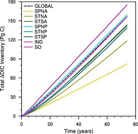
Figure 4. Time series of total dissolved inorganic carbon inventory anomaly against time for the global (dashed) and different regional (solid) ocean alkalinity enhancement experiments.
The same mass of alkalinity is added to each region; however, the actual impact of the alkalinity enhancement on surface TA concentrations depends on the area size of each region (Table 1). For example, the carbon uptake in the Global OAE experiment, which has the largest surface area and lowest input concentrations, is exceeded only by the SO and SPNP regional experiments, which have the second and third smallest surface areas and highest input concentrations of the regional experiments. However, the SPNA region, which has the smallest area and highest input concentration, sequesters the least CO2 over the course of the experiment. Therefore, neither the surface area of the input region nor the subsequent input concentration directly regulates the carbon-uptake potentials between experiments.
The availability of the additional TA in the surface, where it influences the carbon-uptake potential, is controlled by the different hydrodynamic regimes between the selected regions. We refer to the total surface availability of enhanced alkalinity after vertical export as surface retention. The evolution of the total mean depth profile through time illustrates the influence of vertical export to surface retention (Supplementary Figure 1). The range of surface retention varies from the SPNP experiment, with the greatest total TA anomaly of 0.73 Pmol, to the SPNA, which exhibits the smallest total TA anomaly of 0.12 Pmol (Figure 5A). The increase of the total surface TA anomaly in each experiment is non-linear with a greater rate of increase initially, which decreases over the simulation period. The growth rates of the total surface TA anomaly for the Subtropical North Pacific (STNP) and Subtropical South Pacific (STSP) regional simulations are near-linear after an initial rate decrease. The Indian Ocean (IND), SPNP, STNP and STSP regions exhibit greater total surface TA anomalies after 75 years than the Global experiment, while only the SPNP and IND regions exceed the carbon-uptake in response to Global OAE. The surface retention of TA after 75 years of Global alkalinity enhancement (0.48 Pmol) also exceeds that of the SO experiment (0.34 Pmol). The total surface availability of TA, therefore, does not determine the carbon uptake response in our experiments.
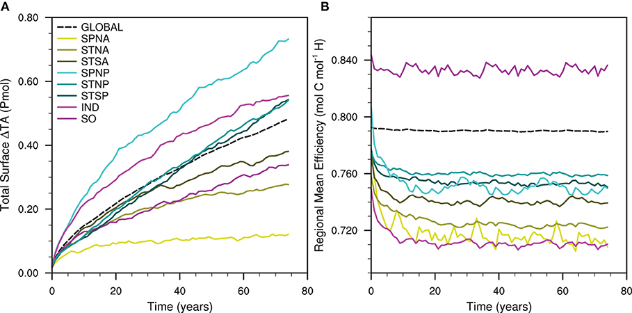
Figure 5. Time series of (A) the total surface total alkalinity anomaly and (B) the carbon-uptake efficiency (Renforth and Henderson, 2017) over time for the global and regional artificial ocean alkalinity experiments.
Renforth and Henderson (2017, Equation 11) illustrate that carbon uptake is influenced by the mean ratio of ΔDIC to ΔTA, which we refer to as carbon-uptake efficiency. The carbon-uptake efficiencies of the Global and regional OAE experiments decrease at different rates over time in response to alkalinity enhancement (Figure 5B). The SPNA region displays the largest decrease of –0.069 mol C mol-1 H+ and the Global shows the least decrease of –0.007 mol C mol-1 H+. The SO carbon-uptake efficiency remains greater than that of the Global experiment throughout the 75-year simulation. While the SPNP initially has a carbon-uptake efficiency greater than the Global, the carbon-uptake efficiency declines in the first 5–10 years to efficiencies comparable with those of the STNP and STSP regions for the remainder of the experiment. This initial rate of decrease within the first 5–10 year period is present in all of the regional OAE simulations. We find no correlation between the regional mean carbon-uptake efficiency (Figure 5B) and the total DIC inventory anomalies (Figure 4).
Neither the surface retention of TA nor the regional carbon-uptake efficiency are found to be predictors of the carbon uptake response to OAE. If the additional TA is retained in the input region then the total DIC inventory anomalies should be a function of the surface TA anomalies and the regional mean carbon-uptake efficiency. However, as this is not case, it indicates that there is horizontal export of additional TA from the input region. Therefore, the surface TA anomalies are not confined to the input regions and the significance of the surface redistribution must be considered.
3.2. Influence of Total Alkalinity Surface Distribution on Carbon Uptake
The influence of the TA distribution in the surface ocean is evident when comparing the simulated (Figure 4) and predicted total DIC inventory changes, for example in the Global and Southern Ocean (SO) alkalinity enhancements. More carbon is sequestered over the course of the simulation in the SO than in the Global OAE experiment despite the SO having smaller surface TA anomalies (Figure 5A). While the Global region has a lower carbon-uptake efficiency (Figure 5B), this is insufficient to explain the response observed. If the surface TA anomalies (Figure 5A) are totally retained within the input regions and the input regions take up carbon at the regional mean carbon-uptake efficiencies (Figure 5B), then the Global experiment would be expected to sequester 213 PgC after the 75 years. In the same scenario, we would expect 162 PgC to be sequestered by the end of the SO experiment. Therefore, the simulated total DIC inventory changes for the Global experiment is less efficient than those predicted, while the SO experiment is more efficient (Figure 4); these divergences are attributed to the export of additional alkalinity from the input regions.
We illustrate this horizontal export of additional TA with the proportion of total surface TA anomalies which remain within the input region. The percentage of the total surface TA anomaly present within the input region for each experiment decreases non-linearly over time (Figure 6). The Global OAE simulation exhibits the greatest proportion of the total surface TA anomaly within the defined input region by the end of the experiment. However, within the first 2 years, the Subtropical South Atlantic (STSA) and Subtropical South Pacific (STSP) regions display greater proportions than the Global. The STSA and STSP also show the largest changes in proportion after 75 years, while the smallest change occurs in the Subpolar North Atlantic (SPNA) experiment. At the end of the simulation, the Subtropical North Atlantic (STNA) has the greatest proportion of total surface TA anomaly, while the SO is found to have the least out of the different regional OAE simulations. We find that the horizontal and vertical export of additional TA from the surface input region varies dependent upon the prevailing hydrodynamic regimes.
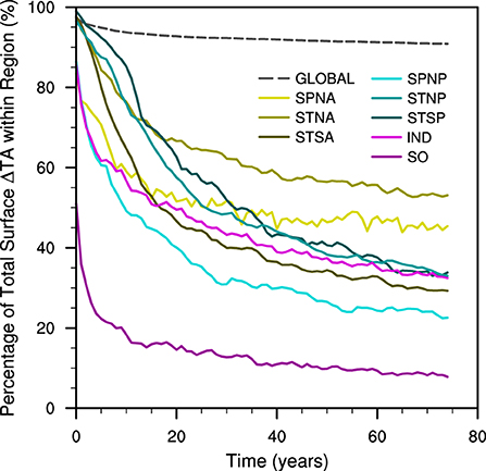
Figure 6. Time series of the percentage of total surface total alkalinity anomalies within the defined region over time for the global and different regional ocean alkalinity enhancement experiments.
The patterns of surface and vertically-integrated TA anomalies from the Global experiment give insight into the mechanisms that distribute alkalinity across the surface ocean and to depth. The annual mean surface TA anomalies are heterogeneously distributed at the end of the 75 year Global OAE simulation, with higher concentrations at subtropical latitudes (Figure 7A). The smallest annual mean surface TA anomalies are found outside the input region, with greater invasion of TA to the Arctic Ocean than south of the seasonally ice-covered areas in the Southern Ocean. Smaller annual mean surface TA anomalies also occur in the eastern subtropical Atlantic and Pacific and in the eastern tropical Pacific. Similar annual mean surface TA anomaly features are present in the western subpolar Atlantic and Pacific. The vertically-integrated TA anomalies are also heterogeneously distributed, with the greatest anomalies occurring within the Arctic Ocean (Figure 7C). The vertically-integrated TA anomalies within the North Atlantic are greater than those of the other major ocean basins. There is an increasing east-west gradient in the vertically-integrated TA anomalies of the subtropical and equatorial regions, while the subpolar North Pacific has an inverse gradient, increasing west to east.
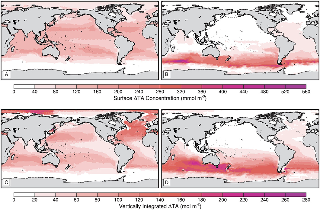
Figure 7. Maps of (A,B) surface total alkalinity anomaly and (C,D) vertically-integrated total alkalinity anomaly for the (A,C) Global and (B,D) Southern Ocean ocean alkalinity enhancement experiments.
The distributions of surface and vertically-integrated TA anomalies differ considerably in the SO experiment compared with the Global. At the end of the 75 year simulation, the annual mean surface (Figure 7B) and vertically-integrated TA anomalies (Figure 7D) dominate the southern subpolar and subtropical latitudes with minor anomalies found in regions of the northern hemisphere. The greatest annual mean surface TA anomaly is found in the Indian Ocean sector of the SO region, while the greatest vertically-integrated anomaly is located in the South Atlantic. Surface TA anomalies are present in the northern Indian Ocean and North Atlantic, however the feature in the Indian ocean is not contiguous with other surface TA anomalies. The low surface TA anomalies displayed by the southern subtropical Indian Ocean appear to continue south around the African coastline to the South Atlantic. The disconnection of the northern Indian Ocean surface TA anomalies is not shared by the vertically-integrated TA anomalies. Large vertically-integrated TA anomalies occur in the southern subtropical Indian Ocean and Tasman Sea. The Arctic Ocean and the North Atlantic Ocean also display small vertically-integrated TA anomalies which are not apparent in the surface distribution of TA anomalies. There are no apparent east-west gradients of vertically-integrated TA anomalies across the southern subtropical regions in the SO OAE experiment such as those in the same regions of the Global.
The greater CO2 sequestration exhibited by the SO compared to the Global OAE simulation is likely the result of the different surface TA anomaly distributions across regions of varying carbon-uptake efficiency. The patterns of annual mean surface and vertically-integrated TA anomalies for all of our experiments are illustrated in Supplementary Figures 2, 3. For comparability, we now consider the regional mean carbon-uptake efficiencies and patterns of surface TA anomalies and TA inventory anomalies with respect to the major ocean basins (Table 2) as defined by the International Hydrographic Organization (IHO; 1953). At the end of the SO simulation, there are greater proportions of the surface TA anomalies present in the South Atlantic and South Pacific, which exhibit greater regional mean carbon-uptake efficiencies than the North Atlantic and North Pacific. In contrast, the Global experiment displays greater proportions of surface TA anomalies in the less efficient North Atlantic and North Pacific (Table 2).
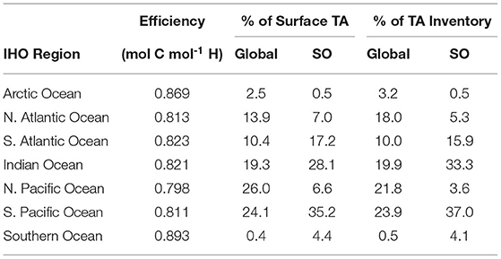
Table 2. Major oceans following International Hydrographic Organization region definitions, their mean carbon-uptake efficiency and the percentage of total surface total alkalinity anomaly and total alkalinity inventory anomaly within the region for the Global and Southern Ocean (SO) ocean alkalinity enhancement experiments.
Carbon uptake is constrained by transport of added alkalinity through horizontal advection to regions which inhibit CO2 uptake and by vertical convection away from the ocean surface. The Southern Ocean and Arctic Ocean display the greatest regional mean carbon-uptake efficiencies (Table 2). However, due to the influence of seasonal or permanent sea-ice cover, which is assumed in HAMOCC6 to prevent CO2 uptake (Ilyina et al., 2013a), TA exported to the Southern Ocean and Arctic Ocean has a negligible influence on carbon uptake. The larger proportion of TA inventory relative to the surface TA present in the North Atlantic after 75 years in the Global simulation (Table 2) illustrates the removal of TA from the surface by seasonal deep convection (Lazier et al., 2002; Sayol et al., 2019). The withdrawal of TA from the surface reduces how much additional TA is available to increase the buffering capacity and enhance the carbon-uptake potential in the North Atlantic. In the Global experiments, this presents a trap for the added alkalinity that has less impact in the SO alkalinity enhancement due to the pattern of surface TA (Figure 7).
3.3. Impact of Ocean Alkalinity Enhancement on Alkalinity Sensitivity
The total marine carbonate system becomes less sensitive to TA in all of our alkalinity enhancement experiments. The total mean alkalinity sensitivity increases non-linearly with respect to the total mean surface TA, where the rate of increase displays varying rates of decline between the different simulations (Figure 8A). The Southern Ocean (SO) OAE experiment has the lowest total annual mean alkalinity sensitivity which increases by 0.03 in the first year and increases at a slower rate in the following years. The greatest total mean alkalinity sensitivity (-8.51) occurs in the Indian Ocean (IND) simulation. The Subpolar North Atlantic (SPNA) and Subtropical North Atlantic (STNA) OAE experiments do not exhibit decreases in the alkalinity sensitivity growth rate within the range of surface TA simulated.
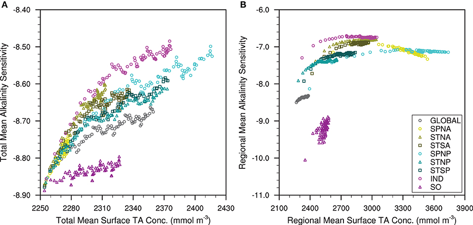
Figure 8. (A) The total annual mean surface alkalinity sensitivity against the total annual mean surface total alkalinity and (B) the regional annual mean surface alkalinity sensitivity against the regional annual mean surface total alkalinity for the global and different regional ocean alkalinity enhancement experiments.
The marine carbonate system also becomes less sensitive regionally in all experiments except for the SPNA alkalinity enhancement, where sensitivity increases. The regional mean alkalinity sensitivities vary non-linearly with respect to the regional mean surface TA, where alkalinity sensitivity increases to a plateau in all of the OAE simulations, except for the SPNA and SO (Figure 8B). The SO exhibits the greatest increase of regional mean alkalinity sensitivity (+1.16) with the smallest range of regional mean surface TA (230 mmol m-3) of the regional experiments. The IND, STNA and Subtropical North Pacific (STNP) OAE simulations exhibit similar increases of regional mean alkalinity sensitivity (0.58-0.60) at different magnitudes of alkalinity sensitivity. The STNA and STNP OAE simulations exhibit smaller increases of regional mean alkalinity than the Subtropical South Atlantic (STSA) or Subtropical South Pacific (STSP), respectively. The regional mean alkalinity sensitivity for the SPNA initially increases to a maximum of –6.90 with a regional annual mean surface TA of 2966 mmol m-3 before decreasing below the initial sensitivity to –7.24 at the end of the simulation.
4. Discussion
4.1. Drivers of the Marine Carbonate System Response to Alkalinity Enhancement
The physical regimes within MPIOM, which drive the distribution of added alkalinity, represent real-world processes but are resolved with biases resulting from implementation, resolution and parameterisation choices (Jungclaus et al., 2013). The distribution of surface TA anomalies in the Global experiment (Figure 7A) is attributed to the pattern of prescribed freshwater fluxes (i.e., evaporation/ precipitation; Middelburg et al., 2020) and the resolved wind-driven circulation (Knauss, 2005). Surface TA is concentrated at subtropical latitudes by prevailing evaporation and anticyclonic gyre circulation (Figure 7A). Surface water is transported toward gyre cores, near the relative western boundaries, where it is forced downward by Ekman Pumping (Knauss, 2005); downward advection of added alkalinity produces the vertically-integrated TA anomalies in the western subtropics (Figure 7C). The downwelling circulation at subtropical latitudes is balanced by coastal upwelling, which raises deeper water (Knauss, 2005) without alkalinity enhancement to the surface, leading to the low anomalies displayed in Figure 7A. TA transported by surface currents into the Arctic Ocean (Karcher et al., 2012; Rudels, 2015) is trapped at depth by thermohaline convection, which leads to the contrast between the relatively large vertically-integrated TA anomalies and the relatively small surface TA anomalies. The divergence of upwelling water masses at the subpolar front of the Southern Ocean (van Heuven et al., 2011; Sévellec et al., 2017) inhibits the southward invasion of TA in the Global OAE simulation and produces the northward transport of TA exhibited by the Southern Ocean (SO) experiment. We show that the redistribution of additional TA is driven by physical circulation and ventilation and, therefore, is model dependent.
While the physical regimes drive the distribution of added alkalinity, the background state of the carbonate system drives the different local responses to OAE. Note that the increases visualised in Figure 8 represent a decrease of the pCO2 reduction per mole of TA added (Sarmiento and Gruber, 2006) and, subsequently, the system is less sensitive to further TA input. The increase of the total mean alkalinity sensitivity (Figure 8A) is attributed to the enhanced sequestration of CO2 due to OAE, which dissociates to introduce further hydrogen ions. These counter the TA input and additional TA is then required to produce an equivalent change of the oceanic pCO2. This effect, and the resulting change in sensitivity, is enhanced by the prescription of the atmospheric CO2 mixing ratio. OAE reduces the atmospheric CO2 growth rate in ESMs with interactive atmospheric CO2 mixing ratios (Keller et al., 2014; González and Ilyina, 2016; Lenton et al., 2018), weakening the atmosphere-ocean concentration gradient. The decreased rate of change of the alkalinity sensitivity is related to the DIC:TA ratio. Egleston et al. (2010) illustrate that seawater buffer factors approach minima, where DIC:TA ratios approach one. The SO OAE simulation exhibits the highest DIC:TA ratio and the smallest change in total mean alkalinity sensitivity (Figure 8A). In contrast, the Indian Ocean (IND) experiment displays the lowest DIC:TA ratio and the greatest change in total mean alkalinity sensitivity. The wider implications of these responses suggest that when the rate of TA input exceeds the rate of carbon uptake, hydrogen ion concentrations become increasingly small. There are fewer hydrogen ions to be neutralised by additional alkalinity enhancement and, therefore, an increasingly weak impact on the atmosphere-ocean CO2 concentration gradient (Zeebe and Wolf-Gladrow, 2003; Middelburg et al., 2020).
We show that physical regimes, which control patterns of TA and DIC, in combination with the non-linearity of buffer factors (Egleston et al., 2010) drive the regional alkalinity sensitivity response to OAE. The regional mean surface TA anomalies are inhibited in the SO region by the surface current connections to the Atlantic, Indian and Pacific Oceans. The Subpolar North Atlantic (SPNA) however, is constrained by land boundaries with limited connections to the Arctic Ocean and North Atlantic but experiences stronger seasonal vertical mixing/ diffusion due to wind stress than regions at lower latitudes (Kara et al., 2003). This seasonal vertical mixing/ diffusion drives the removal of TA and DIC from the surface ocean in the SPNA region (Supplementary Figures 2C, 3C). This permits the accumulation of the TA tracer and strong carbon uptake when the seasonal mixed-layer depth is shallow and the strong reduction of the surface signal with the seasonal deepening of the mixed-layer. The decreasing regional mean alkalinity sensitivity at high regional mean surface TA (Figure 8B) is likely due to the relatively low surface DIC concentrations. This occurs as the TA input rate is greater than the carbon uptake leading to lower DIC:TA ratios. In comparison, we consider that this does not occur in the Subpolar North Pacific (SPNP) region, which also exhibits high regional mean surface TA, because the SPNP experiences weaker vertical turbulent mixing/ diffusion. TA and DIC accumulate in the shallow surface mixed layer of the SPNP region, leading to a higher DIC:TA ratio (Supplementary Figures 2B, 3B). The surface concentrations of DIC and TA produce a lower regional mean alkalinity sensitivity in the SPNA than the SPNP (Figure 8B), despite the local DIC:TA ratios, due to the non-linear buffer factor responses (Egleston et al., 2010).
4.2. Comparisons of Modelled Regional Ocean Alkalinity Enhancement
The CO2 sequestration of the Global OAE experiment is greater than expected from the results of Keller et al. (2014) or Lenton et al. (2018); this is likely due to the different representation of physical and biogeochemical processes in the different models. The total integrated DIC inventory change of the Global OAE experiment (+156.9 PgC; Figure 4) is greater than that of the global OAE simulation of Lenton et al. (2018) under the RCP2.6 scenario (+143.1 PgC). This is unexpected because Lenton et al. (2018) show that under the same OAE application, more CO2 is sequestered at higher atmospheric CO2 concentrations. Lenton et al. (2018) and Keller et al. (2014) find comparable total integrated DIC inventory changes under the RCP8.5 scenario, despite implementing different ESMs. The respective ESMs with their divergent process representations under transient climate scenarios are substantially different from the idealised ocean-only MPIOM-HAMOCC with prescribed pre-industrial climate. For instance, feedbacks between the ocean and other components of the climate system are absent in our set-up.
Beyond the variations of structure, formulation and resolution between models used in OAE studies, the physical and biogeochemical conditions of the pre-industrial climate-state are likely to be more sensitive to OAE than the present or predicted future climate-states. The pre-industrial climate-state (section 2.3) exhibits lower surface water temperatures and, respectively, greater CO2 solubilities than the 21st century simulations conducted by Keller et al. (2014) and Lenton et al. (2018), which would be expected to enhance carbon uptake. Additionally, while wind-driven surface circulations have not changed significantly with climate change, enhanced ocean stratification is weakening vertical mixing (Bindoff et al., 2019); it is not clear to what extent these differences are resolved between the different models. Furthermore, the sensitivities of the marine carbonate system are expected to decrease with ongoing anthropogenic climate change (Egleston et al., 2010; Lenton et al., 2018), which increases the mass of TA required to produce the same response in the marine carbonate system.
The fixed atmospheric CO2 mixing ratio in this study, in contrast to studies using ESMs with emission scenarios, limits the transferability of our findings to the real-world. We cannot directly assess growth rate changes in the atmospheric CO2 mixing ratio in response to OAE, which is a topic of extensive study (Ilyina et al., 2013b; Köhler et al., 2013; Keller et al., 2014; González and Ilyina, 2016; Lenton et al., 2018; Sonntag et al., 2018; Fröb et al., 2020). Furthermore, the assumption of a constant atmospheric CO2 mixing ratio is valid considering that the annual sequestration rates we describe (1.1-2.3 GtC a-1) are lower than both the estimated range of the natural ocean carbon uptake (1.9–3.1 GtC a-1) and anthropogenic emissions (8.9–9.9 GtC a-1) in the present (Friedlingstein et al., 2020).
Previous studies on regional applications of OAE illustrate the sensitivity of carbon-uptake potential to application area and mass of TA added. We find that both the Southern Ocean (SO; +18 PgC) and Subpolar North Pacific (SPNP; +3 PgC) OAE simulations sequester more carbon than the Global, while the Subpolar North Atlantic (SPNA) sequesters less (–75 PgC; Figure 4). Lenton et al. (2018) implement the same TA input rate (section 2.3) but apply TA homogeneously in latitudinal bands without consideration for different physical regimes. Their experiments display similar changes in total integrated carbon uptake for global and regional OAE with little sensitivity to the OAE application region (Lenton et al., 2018). In contrast, Ilyina et al. (2013b) describe TA experiments designed to counter CO2 emissions with a relative TA input rate. A CO2 drawdown by regional OAE equivalent to a global application is illustrated, when TA is added to both the North Atlantic and North Pacific. Their results indicate a sensitivity to the OAE application region and also reveal a weaker CO2 sequestration by regional OAE in the subpolar North Atlantic compared to the subpolar North Pacific or Southern Ocean (Ilyina et al., 2013b). The homogeneous distribution of TA in subpolar latitudes by Lenton et al. (2018) may have reduced the effectiveness of the regional application due to the weaker response of the SPNA compared with other subpolar regions described here and by Ilyina et al. (2013b).
4.3. Implications for Future Ocean Alkalinity Enhancement Studies
While HAMOCC6 resolves biological processes which influence TA (Ilyina et al., 2013a), there are no mechanisms by which the addition of the implemented conceptual TA tracer can directly affect the biological compartments. OAE influences environmental conditions such as increased calcite saturation states and pH (Feng et al., 2017; Renforth and Henderson, 2017; Gore et al., 2019) and indirectly impacts others, such as trace metal concentrations (Hartmann et al., 2013; Köhler et al., 2013) including iron. In some regions, elevated concentrations of iron in the surface ocean may have a fertilising effect on oceanic phytoplankton, which could subsequently enhance the biological carbon pump (Köhler et al., 2013; Bach et al., 2019). However, unlike anthropogenic ocean acidification, where the effects on biota, ecosystems and human communities are undergoing continual research (Doney et al., 2020), the consequences of alkalinity enhancement (Bach et al., 2019; Gore et al., 2019) are less frequently investigated. Therefore, due to sparse information, bulk phytoplankton, cyanobacteria and zooplankton are implemented within HAMOCC6 with constant mortality rates and cannot respond to extremes of biogeochemical variables (Ilyina et al., 2013a) such as those which occur in the subpolar regional OAE simulations.
In its present state, HAMOCC6 has only limited potential to explore biological feedbacks resulting from OAE. An explicit representation of alkalinity-enhancing minerals (e.g., olivine or lime) as tracers in the model would provide additional details related to the Earth system response to OAE. The implementation of bulk phytoplankton, cyanobacteria and zooplankton in HAMOCC6 cannot resolve community assemblage shifts in response to ocean acidification or alkalinity enhancement (Beszteri et al., 2018; Hoppe et al., 2018; Taucher et al., 2018); however, it can still be used to test the "white or green ocean hypothesis" described by Bach et al. (2019). This hypothesis suggests that lime-based OAE would benefit carbonaceous species (i.e., coccolithophores), leading to a whitening of the ocean-colour. In contrast, an olivine-based OAE scenario would benefit siliceous species (i.e., diatoms) and iron-limited but not nitrogen-limited production by cyanobacteria, leading to a greening (Bach et al., 2019). Furthermore, the representative tracers could be used to test their different carbon-uptake potentials with respect to a variable biological carbon pump beyond the previous works of Keller et al. (2014), González and Ilyina (2016), and Lenton et al. (2018).
The response of regional OAE is expected to evolve with changing climate due to physical feedbacks in the climate system. The weakening of buoyancy-loss driven overturning circulations predicted by ESM simulations (Bindoff et al., 2019) could reduce the strong seasonal surface removal in the Subpolar North Atlantic (SPNA) and enhance the effectiveness of OAE. Furthermore, with the assumption of sea-ice impermeability to gas exchange (Ilyina et al., 2013a), reduced sea-ice extents and concentrations due to climate change (Meredith et al., 2019) could enhance carbon uptake in high-latitude regions where the added TA is transported to current seasonally or permanently ice-covered regions. The dependence of the marine carbonate system on temperature and salinity, which evolve with climate (Bindoff et al., 2019), would also be expected to modify biogeochemical sensitivities to OAE over time.
The short duration of most OAE simulations does not illustrate the long-term climate system response, limited studies suggest an acceleration of anthropogenic climate change with the cessation of OAE. The relatively short simulation period (75 years) is comparable with previous regional and global OAE simulations (Ilyina et al., 2013a; Keller et al., 2014; González and Ilyina, 2016; Lenton et al., 2018; Sonntag et al., 2018). These durations are suitable for testing immediate mitigation of the atmospheric CO2 mixing ratio but provide very limited information relating to the response of the ocean interior or long-term effects on the climate system. The sequestration of carbon to the deep ocean has the potential to trap the carbon on centennial-millennial timescales due to deep-ocean ventilation times (Khatiwala et al., 2012). Previous studies of the long-term effects of alkalinity enhancement and the termination of alkalinity enhancement indicate a climate system response of accelerated warming and acidification (González et al., 2018). This suggests that the sequestered CO2 is not contained within centennial-millennial reservoirs during such short-term alkalinity enhancement experiments.
5. Summary and Conclusions
The purposes of this study have been: first, to quantify the influence of regional, in contrast to global, deployments of OAE on CO2 sequestration; and second, to analyse the impact of OAE on the alkalinity sensitivity in different global and regional experiments. We considered the regional variations with the underlying assumption that they are driven by differences between the dominant physical regimes and biogeochemical background states. Our analyses were based on experiments of OAE deployments, which were simulated for 75 years in the ocean-only MPIOM-HAMOCC model with a pre-industrial atmospheric forcing. Alkalinity was enhanced globally and in eight distinct regional experiments, which were selected to represent different hydrodynamic regimes.
Carbon uptake of regionally deployed OAE ranged between 82 and 175 PgC compared to the Global, where 157 PgC was sequestered; therefore, regional alkalinity enhancement has the potential to take up greater and lesser masses of carbon than when deployed globally. Between the different OAE experiments, the total mean alkalinity sensitivity increased by 0.09–0.37 with enhanced alkalinity. In contrast, the regional mean alkalinity sensitivities increased by 0.18–1.06 with increasing alkalinity in all experiments, except for the Southern Ocean, which was dominated by internal variability, and the Subpolar North Atlantic, which decreased by a maximum of 0.19 from its initial state. These regional differences are attributed to the prevailing physical circulation, driving the surface distribution of the added alkalinity, and the initial state of the marine carbonate system, as the alkalinity sensitivity is dependent upon the background DIC and TA.
In conclusion, enhancing alkalinity in smaller regions across the ocean's surface has the potential to exceed carbon uptake in response to global implementations, when hydrodynamic regimes are considered.
Data Availability Statement
Primary data and code for this study are stored and made available through the Max Planck Society Publication Repository (https://pure.mpg.de/): http://hdl.handle.net/21.11116/0000-0008-ABCE-0 (Max Planck Society, Munich, 2021). The respective MPIOM and HAMOCC model code (SHA-1 ID: bb6936773b7e41fad177f8a400b7d0bc627663e6) is available on request after agreeing to the MPI-ESM license agreement and registering at the MPI-ESM Users Forum (https://mpimet.mpg.de/en/science/modeling-with-icon/code-availability, Max Planck Institute for Meteorology, Hamburg and Max Planck Society, Munich, 2021).
Author Contributions
DJB provided the major contribution to the formal analysis, investigation, visualization, and writing. DJB, FF, and TI contributed equally toward concept design, methodology, review, editing, and further aspects of the development of this original research. All authors contributed to the article and approved the submitted version.
Funding
This work was funded by the German Science Foundation (DFG) within the Priority Program Climate Engineering: Risks, Challenges, Opportunities (SPP 1689). This project has received funding from the European Union's Horizon 2020 research and innovation programme under grant agreement No. 820989 (COMFORT) and under grant agreement No. 101003536 (ESM2025–Earth System Models for the Future). This work was also supported by the Research Unit TERSANE (FOR 2332: Temperature-related stressors as a unifying principle in ancient extinctions).
Conflict of Interest
The authors declare that the research was conducted in the absence of any commercial or financial relationships that could be construed as a potential conflict of interest.
Acknowledgments
All simulations were performed at the German Climate Computing Centre (DKRZ). We would like to thank Lennart Ramme for the internal review of this manuscript. The data presented in this study is also analyzed for a thesis (Burt, 2019) toward completion of the Masters of Integrated Climate System Science with the Universität Hamburg in association with the Max Planck Institute for Meteorology.
Supplementary Material
The Supplementary Material for this article can be found online at: https://www.frontiersin.org/articles/10.3389/fclim.2021.624075/full#supplementary-material
References
Bach, L. T., Gill, S. J., Rickaby, R. E. M., Gore, S., and Renforth, P. (2019). CO2 removal with enhanced weathering and ocean alkalinity enhancement: potential risks and co-benefits for marine pelagic ecosystems. Front. Clim. 1:21. doi: 10.3389/fclim.2019.00007
Beszteri, S., Thoms, S., Benes, V., Harms, L., and Trimborn, S. (2018). The response of three Southern Ocean phytoplankton species to ocean acidification and light availability: a transcriptomic study. Protist 169, 958–975. doi: 10.1016/j.protis.2018.08.003
Bindoff, N. L., Cheung, W. W. L., Kairo, J. G., Arístegui, J., Guinder, V. A., Hallberg, R., et al. (2019). “Changing ocean, marine ecosystems, and dependent communities,” in IPCC Special Report on the Ocean and Cryosphere in a Changing Climate, eds H.-O. Pörtner, D. C. Roberts, V. Masson-Delmotte, P. Zhai, M. Tignor, E. Poloczanska, et al., Chapter 5 (Cambridge; New York, NY: Cambridge University Press), 447–587.
Burt, D. J. (2019). The Sensitivity of the Marine Carbon Cycle to Regional Artificial Ocean Alkalinisation. Master's thesis, School of Integrated Climate System Sciences, Universität Hamburg.
Chaigneau, A., and Pizarro, O. (2005). Surface circulation and fronts of the South Pacific Ocean, east of 120oW. Geophys. Res. Lett. 32:4. doi: 10.1029/2004GL022070
de Coninck, H., Revi, A., Babiker, M., Bertoldi, P., Buckeridge, M., Cartwright, A., et al. (2018). “Strengthening and implementing the global response,” in Global Warming of 1.5oC. An IPCC Special Report on the Impacts of Global Warming of 1.5oC Above Pre-Industrial Levels and the Related Global Greenhouse Gas Emissionn Pathways, In The Context of Strengthening the Global Response to the Threat of Climate Change, Sustainable Development and Efforts to Eradicate Poverty, eds V. Masson-Delmotte, P. Zhai, H.-O. Pörtner, D. Roberts, J. Skea, J., P. R. Shukla et al. Chapter 4 (Cambridge; New York, NY: Cambridge University Press), 313–444.
DeVries, T., Le Quéré, C., Andrews, O., Berthet, S., Hauck, J., Ilyina, T., et al. (2019). Decadal trends in the ocean carbon sink. Proc. Natl. Acade. Sci. U.S.A. 116, 11646–11651. doi: 10.1073/pnas.1900371116
Dickson, A. G. (1981). An exact definition of total alkalinity and a procedure for the estimation of alkalinity and total inorganic carbon from titration data. Deep Sea Res. A Oceanogr. Res. Papers 28A, 609–623. doi: 10.1016/0198-0149(81)90121-7
Doney, S. C., Busch, D. S., Cooley, S. R., and Kroeker, K. J. (2020). The impacts of ocean acidification on marine ecosystems and reliant human communities. Annu. Rev. Environ. Resou. 45, 83–112. doi: 10.1146/annurev-environ-012320-083019
Dong, S., Sprintall, J., and Gille, S. T. (2006). Location of the Antarctic Polar Front from AMSR-E satellite sea surface temperature measurements. J. Phys. Oceanogr. 36, 2075–2089. doi: 10.1175/JPO2973.1
Egleston, E. S., Sabine, C. L., and Morel, F. M. M. (2010). Revelle revisited: Buffer factors that quantify the response of the ocean chemistry to changes in DIC and alkalinity. Glob. Biogeochem. Cycles, 24:9. doi: 10.1029/2008GB003407
Feng, E. Y., Koeve, W., Keller, D. P., and Oschlies, A. (2017). Model-based assessment of the CO2 sequestration potential of coastal ocean alkalization. Earths Fut. 5, 1252–1266. doi: 10.1002/2017EF000659
Friedlingstein, P., O'Sullivan, M., Jones, M., Andrew, R. M., Hauck, J., Olsen, A., et al. (2020). Global carbon budget 2020. Earth Syst. Sci. Data 12, 3269–3340. doi: 10.5194/essd-12-3269-2020
Fröb, F., Sonntag, S., Pongratz, J., Schmidt, H., and Ilyina, T. (2020). Detectability of artificial ocean alkalinization and stratospheric aerosol injection in MPI-ESM. Earths Fut. 8:18. doi: 10.1029/2020EF001634
González, M. F., and Ilyina, T. (2016). Impacts of artificial ocean alkalinization on the carbon cycle and climate in Earth system simulations. Geophys. Res. Lett. 43, 6493–6502. doi: 10.1002/2016GL068576
González, M. F., Ilyina, T., Sonntag, S., and Schmidt, H. (2018). Enhanced rates of regional warming and ocean acidification after termination of large-scale ocean alkalinization. Geophys. Res. Lett. 45, 7120–7129. doi: 10.1029/2018GL077847
Gore, S., Renforth, P., and Perkins, R. (2019). The potential environmental response to increasing ocean alkalinity for negative emissions. Mitig. Adapt. Strat. Glob. Change 24, 1191–1211. doi: 10.1007/s11027-018-9830-z
Großkopf, T., Mohr, W., Baustian, T., Schunck, H., Gill, D., Kuyprs, M., et al. (2012). Doubling of marine dinitrogen-fixation rates based on direct measurements. Nature 290, 361–364. doi: 10.1038/nature11338
Hartmann, J., West, A. J., Renforth, P., Köhler, P., De La Rocha, C. L., Wolf-Gladrow, D. A., et al. (2013). Enhanced chemical weathering as a geoengineering strategy to reduce atmospheric carbon dioxide, supply nutrients, and mitigate ocean acidification. Rev. Geophys. 51, 113–149. doi: 10.1002/rog.20004
Hoppe, C. J. M., Schuback, N., Semeniuk, D., Giesbrecht, K., Mol, J., Thomas, H., et al. (2018). Resistance of Arctic phytoplankton to ocean acidification and enhanced irradiance. Polar Biol. 41, 399–413. doi: 10.1007/s00300-017-2186-0
Ilyina, T., Six, K. D., Segschneider, J., Maier-Reimer, E., Li, H., and Núñez-Riboni, I. (2013a). Global ocean biogeochemistry model HAMOCC: Model architecture and performance as component of the MPI-Earth system model in different CMIP5 experimental realizations. J. Adv. Model. Earth Syst. 5, 287–315. doi: 10.1029/2012MS000178
Ilyina, T., Wolf-Gladrow, D., Munhoven, G., and Heinze, C. (2013b). Assessing the potential of calcium-based artificial ocean alkalinization to mitigate rising atmospheric CO2 and ocean acidification. Geophys. Res. Lett. 40, 5909–5914. doi: 10.1002/2013GL057981
International Hydrographic Organization (1953). Limits of Oceans and Seas, Vol. 23 of Special Edition, 3rd Edn. Monte Carlo: International Hydrographic Organization.
Jungclaus, J. H., Fischer, N., Haak, H., Lohmann, K., Marotzke, J., Matei, D., et al. (2013). Characteristics of the ocean simulations in the Max Planck Institute Oceam Model (MPIOM) the ocean component of the MPI-Earth system model. J. Adv. Model. Earth Syst. 5, 422–446. doi: 10.1002/jame.20023
Kara, A. B., Rochford, P. A., and Hurlburt, H. E. (2003). Mixed layer depth variability over the global ocean. J. Geophys. Res. 108:15. doi: 10.1029/2000JC000736
Karcher, M., Smith, J. N., Kauker, F., Gerdes, R., and Smethie, W. M. Jr (2012). Recent changes in Arctic Ocean circulation revealed by iodine-129 observations and modeling. J. Geophys. Res. 117:17. doi: 10.1029/2011JC007513
Karl, D., Michaels, A., Bergman, B., Capone, D., Carpenter, E., Letelier, R., et al. (2002). “Dinitrogen fixation in the world's oceans,” in The Nitrogen Cycle at Regional to Global Scales, eds E. Boyer and R. Howarth, Chapter 2 (Dordrecht: Springer), 47–98.
Keller, D. P., Feng, E. Y., and Oschlies, A. (2014). Potential climate engineering effectiveness and side effects during a high carbon dioxide-emission scenario. Nat. Commun. 5:11. doi: 10.1038/ncomms4304
Keller, D. P., Oschlies, A., and Eby, M. (2012). A new marine ecosystem model for the University of Victoria Earth System Climate Model. Geosci. Model Dev. 5, 1195–1220. doi: 10.5194/gmd-5-1195-2012
Khatiwala, S., Primeau, F., and Holzer, M. (2012). Ventilation of the deep ocean constrained with tracer observations and implications for radiocarbon estimates of ideal mean age. Earth Planetary Sci. Lett. 325-326, 116–125. doi: 10.1016/j.epsl.2012.01.038
Knauss, J. A. (2005). Introduction to Physical Oceanography. 2 Edn. Long Grove, IL: Wavland Press, Inc.
Köhler, P., Abrams, J. F., Völker, C., Hauck, J., and Wolf-Gladrow, D. A. (2013). Geoengineering impact of open ocean dissolution of olivine on atmospheric CO2, surface ocean pH and marine biology. Environ. Res. Lett. 8:9. doi: 10.1088/1748-9326/8/1/014009
Köhler, P., Hartmann, J., and Wolf-Gladrow, D. A. (2010). Geoengineering potential of artificially enhanced silicate weathering of olivine. Proc. Natl Acad. Sci. U.S.A. 107, 20228–20233. doi: 10.1073/pnas.1000545107
Lauvset, S. K., Key, R. M., Olsen, A., van Heuven, S., Velo, A., Lin, X., et al. (2016). A new global interior ocean mapped climatology: the 1o x 1o GLODAP version 2. Earth Syst. Sci. Data 8, 325–340. doi: 10.5194/essd-8-325-2016
Lazier, J., Hendry, R., Clarke, A., Yashayaev, I., and Rhines, P. (2002). Convection and restratification in the Labrador Sea, 1990-2000. Deep Sea Res. 49, 1819–1835. doi: 10.1016/S0967-0637(02)00064-X
Lenton, A., Matear, R. J., Keller, D. P., Scott, V., and Vaughan, N. E. (2018). Assessing carbon dioxide removal through global and regional ocean alkalinization under high and low emission pathways. Earth Syst. Dyn. 9, 339–357. doi: 10.5194/esd-9-339-2018
Liu, B., Six, K. D., and Ilyina, T. (2021). Incorporating the stable carbon isotope13C in the ocean biogeochemical component of the Max Planck Institute Earth System Model. Biogeosci. Discuss. [Preprint]. doi: 10.5194/bg-2021-32
Marsland, S. J., Haak, H., Jungclaus, J. H., Latif, M., and Röske, F. (2003). The max-planck-institute global ocean/ sea ice model with orthogonal curvilinear coordinates. Ocean Model. 5, 91–127. doi: 10.1016/S1463-5003(02)00015-X
Matear, R. J., and Lenton, A. (2014). Quantifying the impact of ocean acidification on our future climate. Biogeosciences 11, 3965–3983. doi: 10.5194/bg-11-3965-2014
Mauritsen, T., Bader, J., Becker, T., Behrens, J., Bittner, M., Brokopf, R., et al. (2019). Developments in the MPI-M earth system model version 1.2 (MPI-ESM1.2) and its response to increasing CO2. J. Adv. Model. Earth Syst. 11, 998–1038. doi: 10.1029/2018MS001400
McDougall, T. J., and Barker, P. (2011). Getting started with TEOS-10 and the Gibbs Seawater (GSW) Oceanographic Toolbox. Sydney, NSW: SCOR/IAPSO WG127.
Meredith, M., Sommerkorn, M., Cassotta, S., Derksen, C., Ekaykin, A., Hollowed, A., et al. (2019). “Chapter 3: Polar regions,” in IPCC Special Report on the Ocean and Cryosphere in a Changing Climate, eds H.-O. Pörtner, D. C. Roberts, V. Masson-Delmotte, P. Zhai, M. Tignor, E. Poloczanska, et al. (Cambridge; New York, NY: Cambridge University Press), 203–320.
Middelburg, J. J., Soetaert, K., and Hagens, M. (2020). Ocean alkalinity, buffering and biogeochemical processes. Rev. Geophys. 58:28. doi: 10.1029/2019RG000681
Najjar, R. G., Jin, X., Louachni, F., Aumont, O., Caldeira, K., Doney, S. C., et al. (2007). Impact of circulation on export production, dissolved organic matter, and dissolved oxygen in the ocean: results from Phase II of the Ocean Carbon-cycle Model Intercomparison Project (OCMIP-2). Glob. Biogeochem. Cycles, 21:22. doi: 10.1029/2006GB002857
Olsen, A., Key, R. M., van Heuven, S., Lauvset, S. K., Velo, A., Lin, X., et al. (2016). The global ocean data analysis project version 2 (GLODAPv2) - an internally consistent data product for the world ocean. Earth Sys. Sci. Data 8, 297–323. doi: 10.5194/essd-8-297-2016
Orr, J. C., Najjar, R. G., Aumont, O., Bopp, L., Bullister, J. L., Danabasoglu, G., et al. (2017). Biogeochemical protocols and diagnostics for the CMIP6 Ocean Model Intercomparison Project (OMIP). Geosci. Model Dev. 10, 2169–2199. doi: 10.5194/gmd-10-2169-2017
Paulsen, H., Ilyina, I., Six, K. D., and Stemmler, I. (2017). Incorporating a prognostic representation of marine nitrogen fixers into the global ocean biogeochemical model HAMOCC. J. Adv. Model. Earth Syst. 9, 438–464. doi: 10.1002/2016MS000737
Poli, P., Hersbach, H., Dee, D. P., Berrisford, P., Simmons, A. J., Vitart, F., et al. (2016). ERA-20C: an atmospheric reanalysis of the twentieth century. J. Clim. 29, 4083–4097. doi: 10.1175/JCLI-D-15-0556.1
Renforth, P., and Henderson, G. (2017). Assessing ocean alkalinity for carbon sequestration. Rev. Geophys. 55, 636–674. doi: 10.1002/2016RG000533
Röske, F. (2005). Global Oceanic Heat and Fresh Water Forcing Datasets Based on ERA-40 and ERA-15. Reports on earth system science.
Rudels, B. (2015). Arctic Ocean circulation, processes and water masses: A description of observations and ideas with focus on the period prior to the International Polar Year 2007-2009. Progr. Oceanogr. 132, 22–67. doi: 10.1016/j.pocean.2013.11.006
Sarmiento, J. L., and Gruber, N. (2006). “Carbon cycle,” in Global Biogeochemical Dynamics, Chapter 8 (Princeton, NJ: Princeton University Press).
Sayol, J.-M., Dijkstra, H., and Katsman, C. (2019). Seasonal and regional variations of sinking in the subpolar North Atlantic from a high-resolution ocean model. Ocean Sci. 15, 1033–1053. doi: 10.5194/os-15-1033-2019
Schott, F. A., Xie, S.-P., and McCreary, J. P. Jr (2009). Indian Ocean circulation and climate variability. Rev. Geophys. 47:46. doi: 10.1029/2007RG000245
Sévellec, F., de Verdiére, A. C., and Ollitrault, M. (2017). Evolution of intermediate water masses based on Argo Float displacements. J. Phys. Oceanogr. 47, 1569–1586. doi: 10.1175/JPO-D-16-0182.1
Shetye, S. R., Shenoi, S. S. C., Gouveia, A. D., Michael, G. S., Sundar, D., and Nampoothiri, G. (1991). Wind-driven coastal upwelling along the western boundary of the Bay of Bengal during the southwest monsoon. Continental Shelf Res. 11, 1397–1408. doi: 10.1016/0278-4343(91)90042-5
Six, K. D., and Maier-Reimer, E. (1996). Effects of plankton dynamics on seasonal carbon fluxes in an ocean general circulation model. Glob. Biogeochem. Cycles 10, 559–583. doi: 10.1029/96GB02561
Sonntag, S., Ferrer González, M., Ilyina, T., Kracher, D., Nabel, J. E. M. S., Niemeier, U., et al. (2018). Quantifying and comparing effects of climate engineering methods on the Earth system. Earths Fut. 6, 149–168. doi: 10.1002/2017EF000620
Taucher, J., Arístegui, J., Bach, L. T., Guan, W., Montero, M. F., Nauendorf, A., et al. (2018). Response of subtropical phytoplankton communities to ocean acidification under oligotrophic conditions and during nutrient fertilization. Front. Marine Sci. 5:14. doi: 10.3389/fmars.2018.00330
Taylor, L. L., Quirk, J., Thorley, R. M. S., Kharecha, P. A., Hansen, J., Ridgwell, A., et al. (2016). Enhanced weathering strategies for stabilizing climate and averting ocean acidification. Nat. Clima. Change 6, 402–406. doi: 10.1038/nclimate2882
van Heuven, S. M. A. C., Hoppema, M., Huhn, O., Slagter, H. A., and de Baar, H. J. W. (2011). Direct observation of increasing CO2 in the Weddell Gyre along the Prime Meridian during 1973-2008. Deep Sea Res. Part II Top. Stud. Oceanogr. 58, 2613–2635. doi: 10.1016/j.dsr2.2011.08.007
Vinayachandran, P. N., Shankar, D., Vernekar, S., and Sandeep, K. K. (2013). A summer monsoon pump to keep the Bay of Bengal salty. Geophysical Research Letters, 40:1777–1782. doi: 10.1002/grl.50274
Wu, Y., Hain, M. P., Humphreys, M. P., Hartman, S., and Tyrrell, T. (2019). What drives the latitudinal gradient in open-ocean surface dissolved inorganic carbon concentration? Biogeosciences 16, 2661–2681. doi: 10.5194/bg-16-2661-2019
Wyrtki, K. (1989). “Some thoughts about the West Pacific warm pool,” in Proceedings of the West Pacific International Meeting and Workshop on TOGA COARE, eds J. Picaut, R. Lukas, and T. Delcroix (Nouméa: Institut Français de Recherche Scientifique pour le Développement en Coopération), 99–109.
Keywords: climate change mitigation, carbon cycle, ocean alkalinity enhancement, biogeochemical modelling, alkalinity sensitivity, carbonate system
Citation: Burt DJ, Fröb F and Ilyina T (2021) The Sensitivity of the Marine Carbonate System to Regional Ocean Alkalinity Enhancement. Front. Clim. 3:624075. doi: 10.3389/fclim.2021.624075
Received: 30 October 2020; Accepted: 01 June 2021;
Published: 08 July 2021.
Edited by:
Lennart Thomas Bach, University of Tasmania, AustraliaReviewed by:
Keith Lindsay, National Center for Atmospheric Research (UCAR), United StatesCarolin Regina Löscher, University of Southern Denmark, Denmark
Copyright © 2021 Burt, Fröb and Ilyina. This is an open-access article distributed under the terms of the Creative Commons Attribution License (CC BY). The use, distribution or reproduction in other forums is permitted, provided the original author(s) and the copyright owner(s) are credited and that the original publication in this journal is cited, in accordance with accepted academic practice. No use, distribution or reproduction is permitted which does not comply with these terms.
*Correspondence: Daniel J. Burt, ZGFuaWVsLmJ1cnRAbXBpbWV0Lm1wZy5kZQ==