Information Entropy as Quantifier of Potential Predictability in the Tropical Indo-Pacific Basin

Global warming is posed to modify the modes of variability that control much of the climate predictability at seasonal to interannual scales. The quantification of changes in climate predictability over any given amount of time, however, remains challenging. Here we build upon recent advances in non-linear dynamical systems theory and introduce the climate community to an information entropy quantifier based on recurrence. The entropy, or complexity of a system is associated with microstates that recur over time in the time-series that define the system, and therefore to its predictability potential. A computationally fast method to evaluate the entropy is applied to the investigation of the information entropy of sea surface temperature in the tropical Pacific and Indian Oceans, focusing on boreal fall. In this season the predictability of the basins is controlled by two regularly varying non-linear oscillations, the El Niño-Southern Oscillation and the Indian Ocean Dipole. We compute and compare the entropy in simulations from the CMIP5 catalog from the historical period and RCP8.5 scenario, and in reanalysis datasets. Discrepancies are found between the models and the reanalysis, and no robust changes in predictability can be identified in future projections. The Indian Ocean and the equatorial Pacific emerge as troublesome areas where the modeled entropy differs the most from that of the reanalysis in many models. A brief investigation of the source of the bias points to a poor representation of the ocean mean state and basins' connectivity at the Indonesian Throughflow.

Introduction

In the past decade, our theoretical understanding of the physics of the climate system has advanced in fundamental ways. These advancements proceeded in parallel with model improvements and computing capabilities. Understanding and especially predicting climate change at regional or local scales—the scales that are relevant to society—remains, however, challenging: regional climate change is influenced by the large-scale climate and, at the same time, feeds back to the global scale but these interactions are poorly represented in models.

In this work, we focus on the tropical Pacific and Indian Oceans, where the El Niño Southern Oscillation (ENSO; Bjerknes, 1966, 1969) and the Indian Ocean Dipole (IOD; Saji et al., 1999; Webster et al., 1999) control the largest portions of the variance at interannual scale (Figure 1). They impact key variables of societal relevance, from surface temperature to precipitation and the frequency of extreme events such as tropical cyclones, typhoons and droughts. These climate modes are of the uttermost importance not only for water and food security, but also for global health, as they modulate, for example, malaria occurrences in India (Dhiman and Sarkar, 2017; Anyamba et al., 2019), Indonesia (Kovats, 2000) and Africa (Hashizume et al., 2012; Kreppel et al., 2019). Assessing their potential predictability and quantifying how this predictability is simulated in climate models and projected to change in the future, is a priority.

FIGURE 1

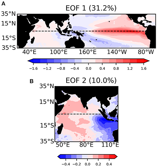
Figure 1. (A) First EOF mode of the tropical Indo-Pacific SST monthly anomalies, showing the observed ENSO pattern. (B) Second EOF mode of tropical Indian Ocean SST monthly anomalies highlighting the IOD patterns. The monthly data cover the period 1980–2018 and are obtained from SODA 3.4.2 reanalysis. Percentages of variance explained by the EOF patterns are included. The black dash line depicts the equator.

ENSO and IOD play a crucial role in global climate variability. In light of this importance, their interactions have been the subject of numerous studies. A recent review of ENSO teleconnections can be found in Yeh et al. (2018). The IOD develops in late summer with a November maximum. Since its discovery, observational and modeling studies have focused on its linkages with the Asian Summer Monsoon (Behera et al., 1999; Ashok et al., 2001; Guan et al., 2003; Saji and Yamagata, 2003), its modulation of the Indian Summer Monsoon and ENSO (Ashok et al., 2001); and its teleconnections over North America, Australia, South-Africa (Li and Mu, 2001) and East Africa (Black et al., 2003). The regional and global influences of these modes cannot be overemphasized, yet a realistic simulation of the characteristics and teleconnections of these modes remains challenging in state-of-the-art climate models (Weller and Cai, 2013), precluding the reliability of future projections.

Here, we introduce the climate science community to a quantifier of complexity, or entropy, recently proposed in the literature that allows for distinguishing regular, chaotic, and random behaviors in time-series. It provides a quick framework to investigate potential predictability and verify how well climate models represent it. We test it using an observationally-based reanalysis product and model data-sets, we verify its robustness and finally use it to exemplify the challenges implicit in using global climate models—here the integrations from the Coupled Model Intercomparison Project phase 5, CMIP5—(Taylor et al., 2012) to investigate present and future predictability. We focus on the Indo-Pacific Ocean in boreal fall, when the IOD variance is maximized and many countries are impacted by its and ENSO modulation of rainfall and temperatures over the surrounding land masses.

The rest of this paper is organized as follows: section Data provides information about the observational data and models used; section The Entropy Quantifier: Recurrence Plots and Information Entropy focuses the information entropy quantifier; sections Entropy in Reanalysis Data, CMIP5 Historical Runs and CMIP5 Projections discusses the entropy of historical and future projection focusing on the boreal fall season, and section Entropy and the ENSO-IOD Relation analyzes possible sources of model bias in the historical period. A summary of the findings concludes the work.

Data

We analyze monthly mean outputs from 15 CMIP5 models and consider both historical runs and future projections following the representative concentration pathway (RCP) 8.5 scenario. For each model, we use at least 1 member for the historical analysis and its evolution in the RCP case. For 10 models we verified that internal model variability does not impact the outcome of our analysis by exploring 3 (or 2 when three runs were not readily available) members in the historical period. The output variable we focus on is sea surface temperature (SST), and further consider sea level pressure (SLP) and thermocline depth (Z20) in investigating model divergence.

In terms of observational datasets, we use the monthly mean subsurface temperature from the Simple Ocean Data Assimilation (SODA) version 3.4.2, which was forced by the European Center for Medium-range Weather Forecasts (ECMWF) re-analysis ERA-Interim (Carton et al., 2018). SODA has a spatial resolution of 0.25° x 0.25° with 50 vertical levels, and spans the 1980- 2017 period. For cross validation, we also considered fields from the Ocean Re-Analysis System 4 (ORAS4) (Zuo et al., 2019). Results obtained using SODA and ORAS4 are nearly identical and consistent. For brevity, we focus our discussion on SODA. Sea level pressure is from the monthly mean ERA-Interim (Dee et al., 2011). All data have been de-trended and re-gridded into a uniform 1° longitude x 1° latitude spatial resolution before analysis. For the observational datasets, we look at the period 1980–2018 for temporal consistency among them, while in the CMIP5 models we consider the last 39 years of the historical period (1967–2005)—same period length as in the reanalyses—and the last 30 years of the XXI century (2071–2100) as representative of future climate. Table 1 summarized the model runs used.

TABLE 1

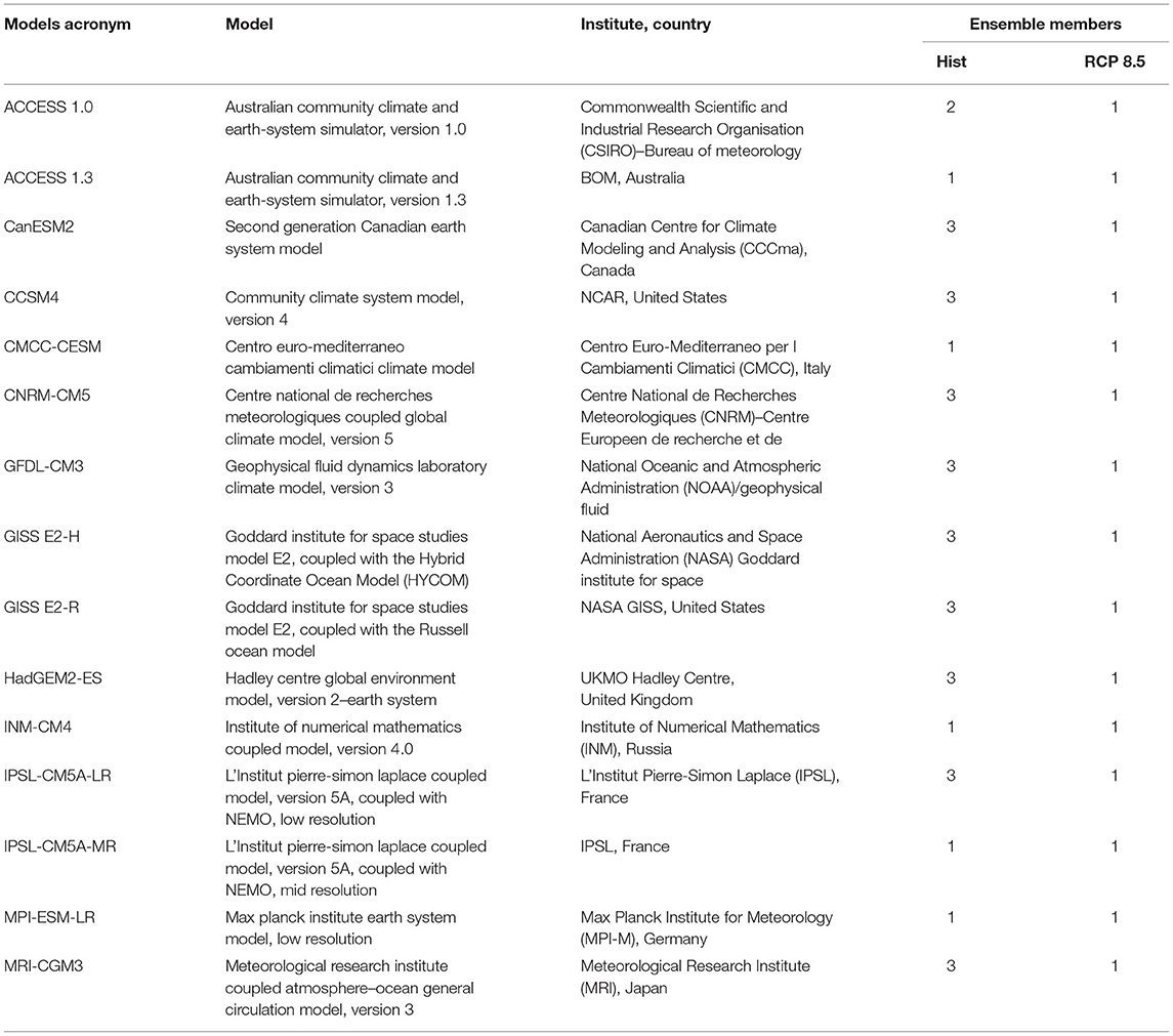
Table 1. Models and ensemble members analyzed in this work.

In the following, the IOD strength and variability is quantified by the IOD Index, which is the difference in the SST monthly anomalies (SSTAs) averaged over the western tropical Indian Ocean (WTIO) (50°–70°E, 10°S−10°N) and in the SETIO region (90°–100°E, 0°S−10°N) (Saji et al., 1999). For ENSO we adopt the Niño-3.4 index, defined as the area-averaged SSTAs over 170°W−120°W, 5°S−5°N. To examine the strength of oceanic linkages between the Pacific and Indian oceans and the relationship between ENSO and IOD, we perform a correlation analysis using the depth anomalies in the 20°C isotherm (Z20), a proxy for the tropical thermocline depth, in the ITF region (area average over 120°E−131.5° E, 7.5°-8.5°S) (Bracco et al., 2005) or the sea level difference between the western Pacific (WP; 0–10°N; 125°E−145°E) and the Eastern Indian Ocean (EIO; 10°S−20°S; 110°E−130°E) (Mayer et al., 2018).

The Entropy Quantifier: Recurrence Plots and Information Entropy

Given a dynamical system, several measures of complexity have been proposed to distinguish regular (e.g., periodic), chaotic and random behaviors in the time-series that describes it. Among those complexity quantifiers, the most common are Lyapunov exponents, fractal dimensions, scaling exponents, divergence rates and entropies (Manneville, 1990; Shi, 2007). Most of these quantifiers work very well in the case of low dimensional dynamical systems but their application is complicated for noisy time series coming from high-dimensional real-world systems. Bandt and Pompe (2002) proposed the permutation entropy quantifier to address this issue, and along with minor modifications this tool has been used in climate science for the analysis of a proxy record of ENSO spanning the Holocene (Saco et al., 2010) and for ice core records by Garland et al. (2019). The permutation entropy depends on two parameters and at least for low dimensional systems (for example a Logistic Map) has a good, but not optimal, correlation with the Lyapunov exponents of the system under investigation.

Here we adopt instead an entropy quantifier based on the distribution of microstates in a recurrence plot (Prado et al., 2020). All complexity quantifiers are based on fundamental phase space properties of ergodic dynamical systems, such as trajectory recurrence (Poincaré, 1890; Cvitanović et al., 2016) and this recurrence can be visualized, for a given time-series, using the recurrence plot (RP) method introduced by Eckmann et al. (1987). Given a trajectory x_i in a dynamical system in its d-dimensional phase space at time i, its RP is given by an N × N matrix of 1 and 0 such as:

$\begin{array}{ll}R{P}_{i,j}\left(\epsilon \right)=\Theta \left(\epsilon -\Vert x_i-x_j\Vert \right),x_i\in {ℝ}^d,i,j=1,\dots ,N& (1)\end{array}$

where ε is the threshold distance and defines the neighborhood of a state x_i, Θ is the Heaviside function, || · || is a norm (Euclidean distance in our case) and N is the number of states considered.

The analysis of structures (such as diagonal, vertical or horizontal lines) in a RP is known as recurrence quantification analysis (RQA) and has found numerous applications in biology, neuroscience, physics, geosciences and economics, among other disciplines (Webber and Marwan, 2015). In essence, given a time series it is possible to reconstruct a state space representation using the embedding theorem (Takens, 1981), and then compute the recurrence plot (which is a matrix with “1” if two states are recurrent, “0” if they are not recurrent). Most methods to estimate complexity of time series are directly related to RQA (Marwan et al., 2007), recurrence network analysis (Donner et al., 2011) and information theory (Bandt and Pompe, 2002; Balasis et al., 2013). Some of these quantifiers have been applied to climate science to analyze regime shifts and tipping points in single time-series (e.g., Donges et al., 2011). All these methods require “phase space reconstruction,” as mentioned, or, in other words, they require embedding the time series in a higher dimensional space. Phase space reconstruction is computationally time consuming and sensitive to both the choice of parameters and to the system's noise and dimensionality (Gilpin, 2020), and is therefore not advisable for real-world spatiotemporal fields as it may lead to spurious results (Marwan, 2011; Riedl, 2013).

To remedy these issues, Corso et al. (2018) proposed a recurrence entropy quantifier that does not require phase space reconstruction and can be safely applied to fields of any dimension and complexity. The idea behind is that the entropy of a time series can be computed by the probability of occurrence of microstates in its RP. A microstate of size M is defined as an M × M matrix inside the RP. The total number of configurations of 1 and 0 in a microstate of size M is M^* = 2^M2 and is possible to define a probability of occurrence P_k of a microstate k as $P_k=\frac{n_k}{M^{\ast }}$, with n_k being the number of occurrences of the k-th microstate in the RP. The information entropy of the time series is then given by:

$\begin{array}{ll}S\left(M^{\ast }\right)=-{\displaystyle \sum _{k=1}^{M^{\ast }}{P}_{k}ln{P}_k}.& (2)\end{array}$

It is possible to normalize the recurrence entropy by its maximum possible value M²ln 2 which corresponds to the case in which all microstates appear with the same probability $P_k=\frac{1}{M^{*}}$; in this case S = 0 (1) implies perfect predictability (unpredictability) of the system dynamics.

The number of admissible microstates M^* grows exponentially as a function of M but Corso et al. (2018) showed that only few of them populate the RP. It is therefore reasonable to consider only a random subsample $\overline{M}$ of the possible microstates in the RP and expect a rapid convergence to S(M^*) (see Supplementary Material). In this case, the entropy is normalized by $ln\overline{M}$.

In layman's terms, the information entropy based on the recurrence of microstates can be computed in two steps by calculating firstly the recurrence plot and then the Shannon Entropy based on the distribution of microstates. If the Euclidean distance between states x(t = a) and x(t = b) is less than epsilon then they are considered neighbors and described by “1” in the recurrence plot matrix, vice versa they are described by “0.”

The recurrence entropy, in whichever way it is calculated, depends on the choice of the distance threshold ε. Several heuristics have been proposed for selecting ε : ~5% of the maximal phase space diameter (Mindlin and Gilmore, 1992); no more than 10% of the mean (or maximum) phase space diameter (Koebbe and Mayer-Kress, 1992; Zbilut and Webber, 1992); a value ensuring a recurrence point density of ~1% (Zbilut et al., 2002). More recently, Prado et al. (2020) relied on the “maximum entropy principle” to free the analysis from having to select ε. Given a RP and microstates of size M, they examined the dependence of the recurrence entropy S on ε and found that, typically, the curve S(ε) has a well-defined maximum, S_Max, that does not vary significantly for a range of ε values. In simple deterministic and stochastic systems, the maximum entropy S_Max calculated by Prado and colleagues is highly correlated with the Lyapunov exponent, further improving the complexity quantifier proposed by Corso et al. (2018). S_Max is therefore our preferred choice. Technical details for the heuristic used to determine it and an example of the convergence when considering only a subsample $\overline{M}$ of all possible microstates in the RP can be found in the Supplementary Material.

The information entropy so computed measures the complexity of the time series examined, and the two terms, entropy and complexity will be used interchangeably in the reminder of the paper. The higher the entropy, the more complex and less predictable is the system, and vice versa. Examples from simple systems such as a logistic map (May, 1976) can be found in both Corso et al. (2018) and Prado et al. (2020). In the Supplementary Material we quantify the information entropy of the Lorenz system (Lorenz, 1963), while a first application to noisy, high-dimensional data can be found in Falasca et al. (2020) in which the authors used the entropy quantifier to identify abrupt regime shifts in paleoclimate simulations.

The information entropy when applied to a climate field quantifies the degree of complexity of a given region (or grid point) and depends only on the size of a microstate M. In the next section we will explore its sensitivity from M = 2 to M = 8. In summary, for a given climate field X(t), in this work we compute the information entropy and its variability for all the time series in the spatial grid to derive the spatiotemporal entropy field S_X(t) without having to rely on embedding.

Entropy In Reanalysis Data, CMIP5 Historical Runs and CMIP5 Projections

The entropy fields for the SST in the SODA/ERA-Interim reanalysis and two representative CMIP5 models, CCSM4 and HadGEM2-ES are shown in Figure 2 using monthly average fields and all months, and for different values of M. With this first analysis we explore the robustness of metric to the size of the microstates. A microstate of size M = 3, for example, quantifies the recurrence between x(t₁), x(t₁+1 month), x(t₁+2 months) and another random sequence x(t₂), x(t₂+1 month), x(t₂+2 months), while if M = 2 the recurrence will be evaluated between x(t₁), x(t₁+1 month) and another, shorter, random sequence x(t₂), x(t₂+1 month), and so on.

FIGURE 2

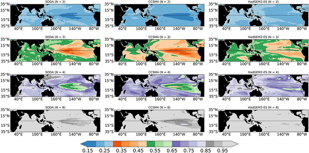
Figure 2. SST entropy fields with microstates, M = 2, 3, 4, and 8 for SODA reanalysis (left column), CCSM4 (middle column) and HadGEM2-ES (right column) CMIP5 historical runs. The data span over the period 1967–2005 for models and 1980–2018 for SODA reanalysis. All months are considered.

The patterns in the entropy plots do not vary significantly with M, but the entropy values do, with generally lower predictability (higher entropy values) and smaller chances of recurrence for increasing M, as to be expected given that we are evaluating the recurrence of a longer (in time) microstate, and very high, unstructured, predictability if M is too small. This dependence can be exploited for studies focusing on different time-scales and output frequency, for example by using daily data for evaluating subseasonal predictability.

When all months are considered, in SODA/ERA-Interim the highest predictability is found in the central tropical Pacific in the ENSO impacted area, as expected. Upwelling regions, both along South America in the cold tongue and in the Arabian Sea, are characterized by higher complexity near the coasts that in offshore waters, and the IOD and SIOD action regions appear slightly more predictable than the remaining IO.

CCSM4 overestimates predictability (underestimates entropy) nearly everywhere. In terms of patterns, it is close to the observed ones, but it does not capture the lower than surrounding predictability of the cold tongue in the Pacific and in the western Arabian Sea upwelling, and underestimates slightly that of the ocean region to the west of the tip of India, that participate in the IOD dynamics. HadGEM2-ES, on the other hand, does not capture the ENSO predictability potential around the Equator (10°N−10°S), and overestimates predictability in the upwelling systems in the Pacific and to the west of Australia.

The usefulness of the entropy is also in highlighting changes in predictability among months, seasons and subseasonal time scales if daily or higher frequency data are available. Given the monthly averages used in this study, we show next the entropy in boreal spring (March to May, MAM) (Figure 3), when complexity is expected to be higher due to the spring predictability barrier to ENSO, and in the extended fall season, August to November (ASON) (Figure 4), when the impacts on the rainfall variability in the continents surrounding the Indian Ocean are greatest and the variance explained by the IOD is largest.

FIGURE 3

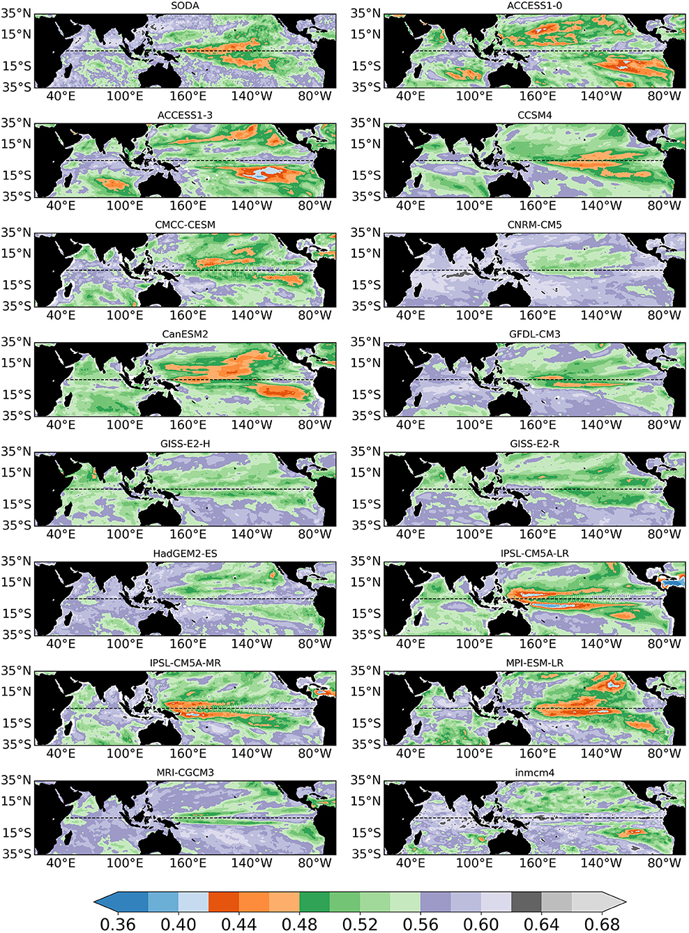
Figure 3. Boreal spring (March–April–May) SST entropy fields with microstates, M = 3 during 1967–2005 for models and during 1980–2018 for SODA reanalysis.

FIGURE 4

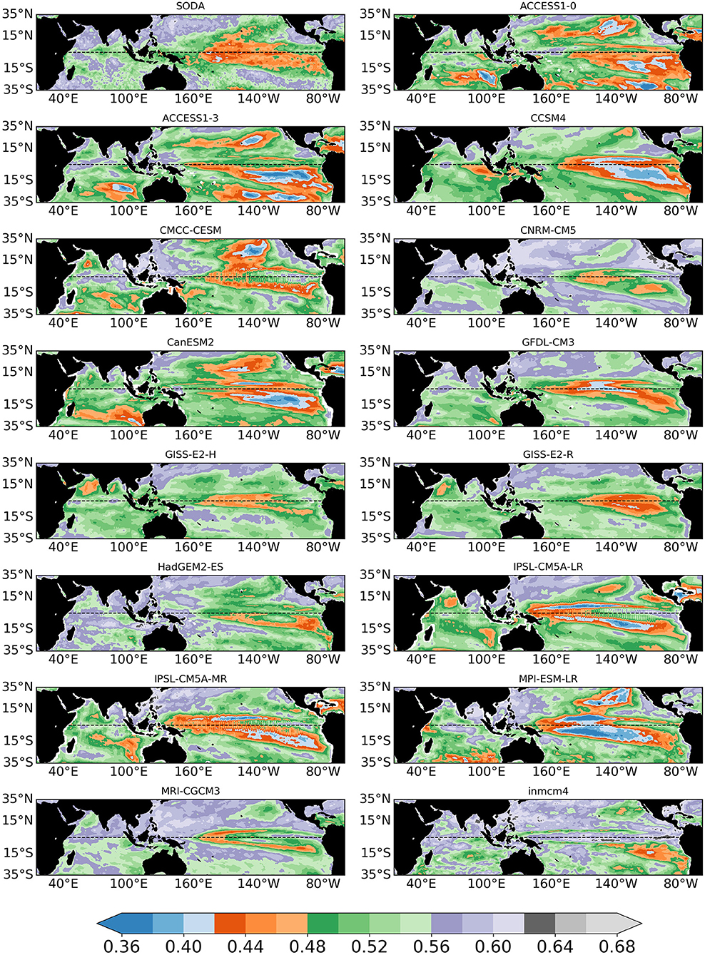
Figure 4. Extended boreal fall (August–September–October–November, ASON) SST entropy fields with microstates M = 3 during 1967–2005 for CMIP5 models and during 1980–2018 for SODA reanalysis.

In both figures the entropy is shown in SODA/ERA-Interim and all models using M = 3, chosen in light of the seasonal scope of our analysis (3 or 4 instead of 12 months in each year). In all CMIP5 models the complexity is higher in boreal spring in the Pacific, indicating that they generally capture the spring barrier to ENSO predictability (e.g., Torrence and Webster, 1998; Duan and Wei, 2013). Little agreement is found among models on the spring predictability of IO.

In boreal fall, models with a realistically shaped—but underestimated—entropy in the ENSO region, especially in the southern hemisphere (CCSM4, CanESM2, MPI) tend to overestimate the predictability in the IO, west of Sumatra for CCSM4 and west of Australia in CanESM2 and MPI. This bias was not as evident in spring. Other models share the bias in the IO but also have high (generally too high) predictability in the tropical Pacific and lower than observed at the equator (ACCESS1.0 and 1.3, CMCC-CESM). CNRM-CM5 reproduces best the entropy patterns in both basins. GFDL-CM3 underestimates the complexity of the equatorial Pacific, while the IPSL model, in both its version, is characterized by an ENSO pattern protruding too far west into the warm pool area and very high predictability north and south of the equator in the western Pacific. The remaining models tend to underestimate the SODA/ERA predictability in the Indo-Pacific. In the IO, many models underestimate the entropy in the 15°S−35°S band and overestimate it along the equatorial ocean, missing the IOD-related predictability and displaying little intra-model agreement on the overall patterns.

Since the IOD discovery, Saji et al. (1999) reported the existence of a correlation between the IOD and ENSO indices. This correlation reaches 0.62 in the ASON season over the period considered for the reanalysis, consistent with the SODA/ERA-Interim entropy pattern, which suggests some predictability potential in the eastern, equatorial and part of the western IO. In the Arabian Sea, on the other hand, the complexity tends to be larger, likely due to the energetic mesoscale field characterizing this upwelling system in fall.

Since correlation does not imply causation, many studies have questioned whether the IOD can occur independently of ENSO and by which mechanism (e.g., Allan et al., 2001; Ashok et al., 2003; Gualdi et al., 2003; Saji and Yamagata, 2003). The general consensus is that the IOD is an ocean-atmospheric coupled mode of climate variability intrinsic to the IO that can be excited by ENSO (see also Webster et al., 1999; Cai et al., 2009). As a result, its predictability does depend on ENSO through an atmospheric teleconnection and possibly through an oceanic bridge. The atmospheric teleconnection is indisputable and is achieved through changes in the Walker circulation over the western Pacific Ocean during the development of ENSO events (e.g., Lau and Nath, 2003; Annamalai et al., 2005; Lau et al., 2005; Behera et al., 2006; Kug et al., 2006; Izumo et al., 2010; Kajtar et al., 2015). Some studies suggest that the ENSO-IOD interaction may also be modulated by an oceanic bridge through changes in the Indonesian Throughflow (ITF) transport between the two basins (Bracco et al., 2005; Yuan et al., 2011; Zhou et al., 2015). The ENSO modulations of the thermocline depth in the Pacific Ocean, and particularly in the Warm Pool region, propagate through the ITF to the northwestern Australia coast and then into the IO (Cai et al., 2005; Behera et al., 2006). The ITF signal is then transported to the southeastern tropical IO (SETIO) by coastal Kelvin waves that develop off south Java (Sprintall et al., 1999). Modeling studies found indeed that closing the ITF annihilates the ENSO-IOD relationship (Wajsowicz and Schneider, 2001; Bracco et al., 2005; Song et al., 2007; Santoso et al., 2011; Kajtar et al., 2015) and van Sebille et al. (2014) confirmed that the ITF transport correlates with ENSO using an eddy-permitting ocean model. In section Entropy and the ENSO-IOD Relation we will briefly investigate these atmospheric and oceanic connections in light of the large discrepancies found among models and between models and reanalysis in the entropy field.

We focus next on future projections. The multi-model mean consensus on the evolution of ENSO under global warming in CMIP5 is toward a strengthening of its amplitude and permanent El-Niño-like conditions (IPCC, 2014; Cai et al., 2015). At the same time the IO warms up but not uniformly. The predicted warming differs significantly among models, but in most the western Indian Ocean warms more than the east side (Di Nezio et al., 2020). In all models but the two versions of GISS-E2, CNRM-CM5 and INMCM4, the warming pattern over the IO resembles that of a positive IOD, which is associated with above normal precipitations over East Africa in fall and greater chances of fires in Australia and Indonesia (not shown). Despite agreement among many models in the warming patterns, no robust behavior is found in the model representation of tropical SST predictability in the RCP8.5 global warming scenarios (Figure 5). In the Pacific, ACCESS1.0, CanESM, IPSL-CM5A-LR are characterized by a decrease in entropy, the opposite is verified in ACCESS1.3, CMCC-CESM, GFDL-CM3, both versions of the GISS model, HadGEM2-ES, IPSL-CM5A-MR, MPI-ESM-LR and INMCM4. The remaining models are almost invariant. In the Indian Ocean the behavior may differ from the Pacific. The entropy decreases in the ACCESS and IPSL runs, all four of them, in CanESM, MRI and in the GFDL model south of the Equator, increases in the CNRM-CM5 run, which had the closest representation to the reanalysis in the historical period, and in the GISS-E2-R model, and is nearly unchanged in the rest of the cases.

FIGURE 5

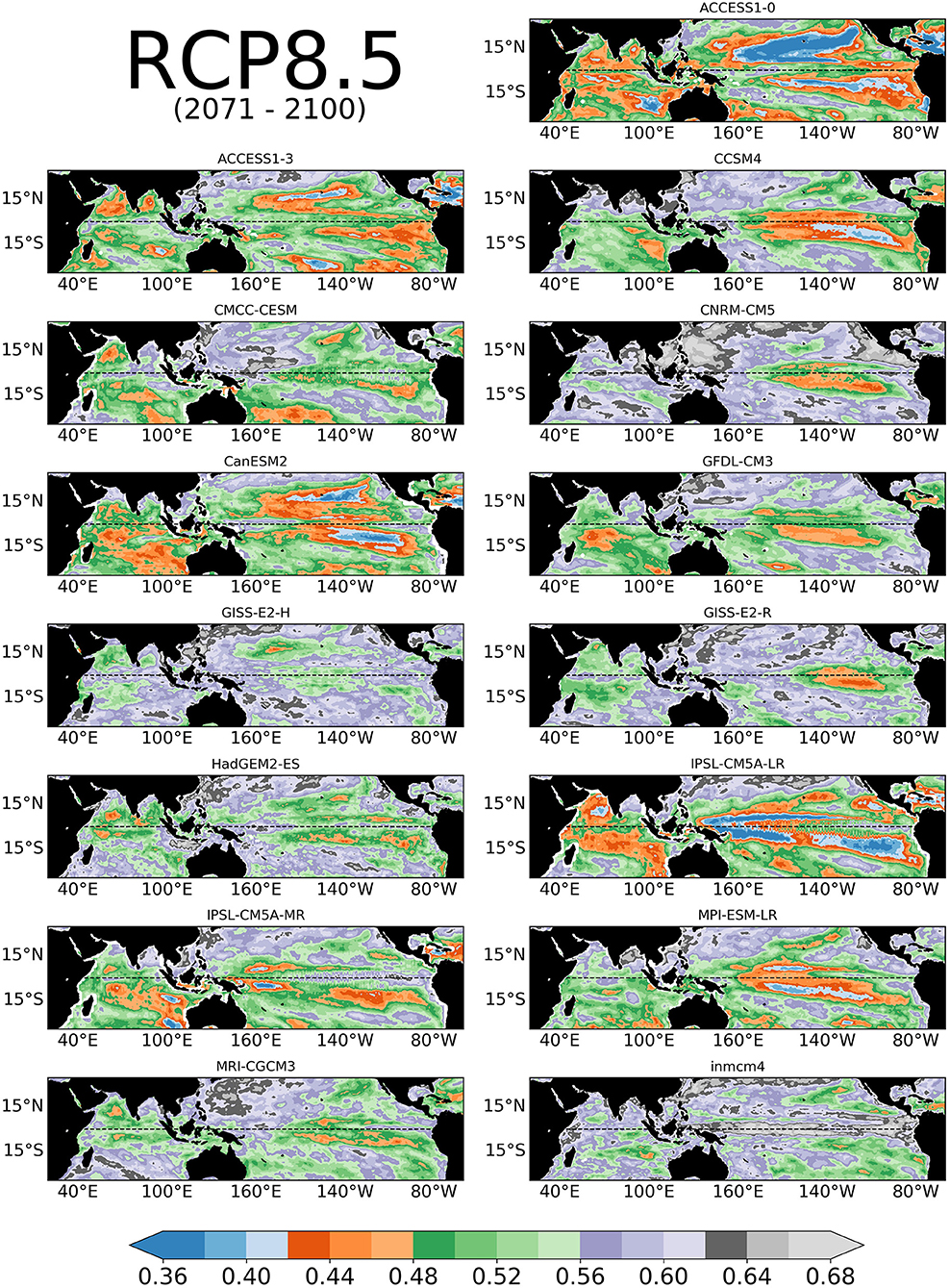
Figure 5. Extended boreal fall (ASON) SST entropy fields with microstates, M = 3 for CMIP5 RCP8.5 runs used in this study. The model data span the period 2071–2100.

The historical and future entropies suggest that many CMIP5 models misrepresent both ENSO and the IOD in boreal fall, and their relationship, and generally underestimate the complexity of the Indian Ocean SST variability, which is neither a mere response to ENSO or independent of it.

Entropy and the ENSO-IOD Relation

In this section, we first discuss how the entropy measure relates to more traditional analysis methods and then we delve into the model biases in the ENSO-IOD representation. We focus on the historical period, for which reanalysis products are available for comparison.

The information entropy is a non-linear time series analysis tool that allow for extracting and accounting for non-linear information that cannot be resolved using traditional linear methods, such as Empirical Orthogonal Function (EOFs), or power spectra. At the same time, the entropy bias can be anticipated in part from a traditional EOF analysis of SST anomalies (Figure 6). Indeed, the entropy identifies major problems in the representation of climate variability patterns, as done by the EOFs, if these biases influence recurrence. Additionally, the information entropy introduces information on the complexity of the climate modes in different regions. Too large complexity in the equatorial Pacific, for example, is indicative of a structural problem common to several models which is not (or not only) linked to the modeled SST ENSO patterns per se, but to the representation of equatorial dynamics both in the atmosphere and in the ocean. The Indo-Pacific EOF patterns are generally more in agreement with reanalysis data than the entropy field. ENSO is often modeled with the observed strength and maximum load at the equator even when it extends too far into the warm pool region (e.g., ACCESS1.3, CCSM4, GFDL, GISS-E2-H, INMCM4, both IPSL versions and MPI) and has too much strength in the central and western portion of the Pacific basin compared to the eastern one (Bellenger et al., 2014; Chen et al., 2017). It is however too strong in CMCC-CESM and CanESM, and too weak in HadGEM2, MRI and INMCM4. In the reanalysis, the SST anomaly patterns in the IO are characterized by a modest negative signal into the SETIO region that extends into the IO from the warm pool region, and by a positive signal elsewhere with slightly larger intensity in the Arabian Sea. The SETIO pattern is often underestimated (this is the case for CanESM and HadGEM-ES, both versions of the GISS and IPSL models), and is stronger than observed but equatorially confined in GFDL. The positive signal, on the other hand, is overestimated in CMCC, GFLD, IPSL and MPI. The EOF patterns, again, do not correspond to the entropy ones, especially south of 15°S, where the SST predictability is often greatly overestimated by the models.

FIGURE 6

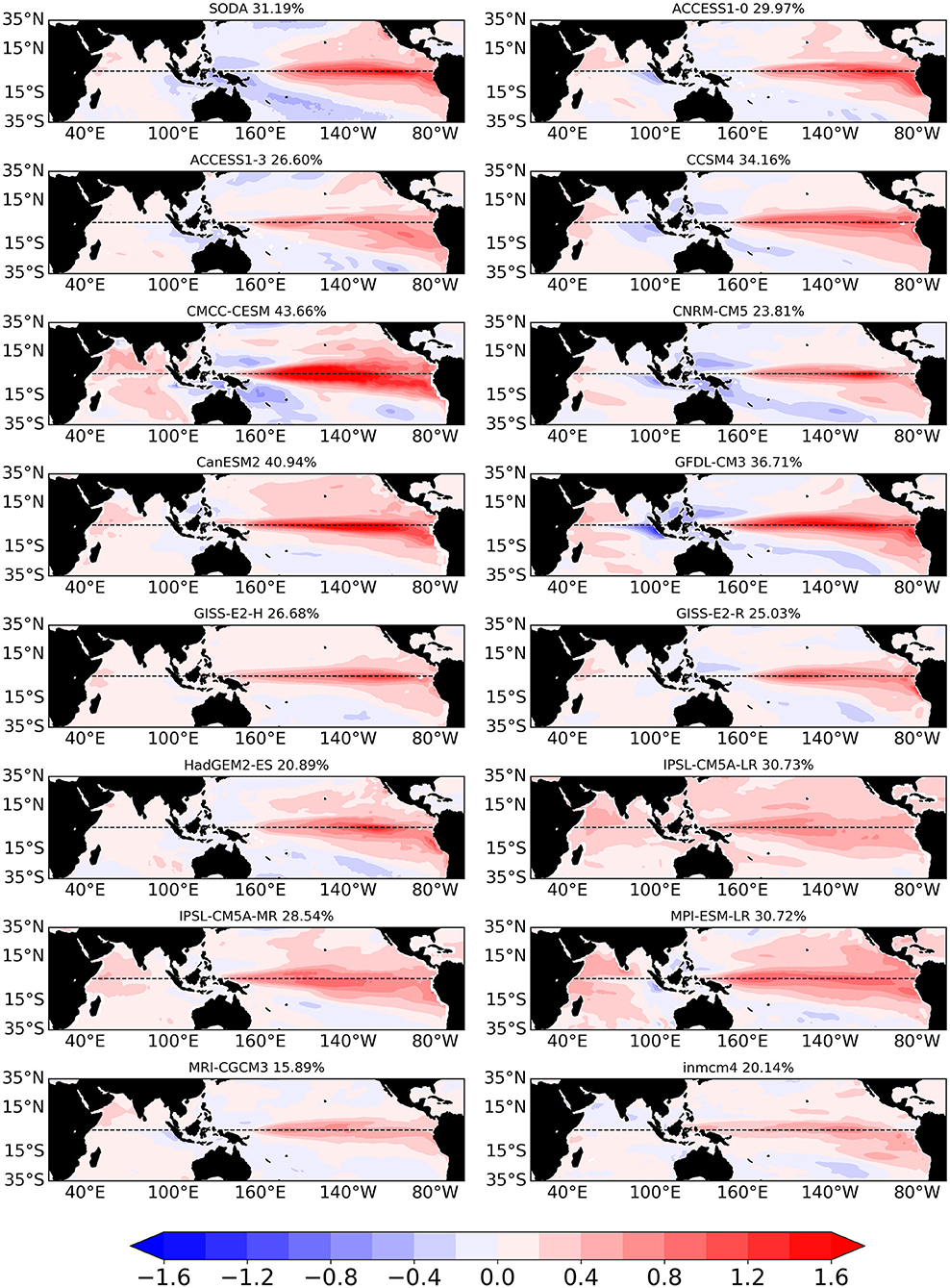
Figure 6. The first EOF patterns of tropical Indo-Pacific sea surface temperature anomalies during the extended boreal fall season (ASON) in 1967–2005 for models and 1980–2018 for SODA reanalysis. Percentages of variance explained by the EOF patterns are included.

The complexity of ENSO is also—but not exclusively—linked to its power spectrum and therefore its periodic recurrence in time. Figure 7 compares the spectra among models and the reanalysis based on the (monthly) Nino3.4 index. The bias in the modeled spectra is reflected in that of the entropy field along the equatorial Pacific, with the caveat that several models overestimate the complexity of ENSO at the equator but display highly predictable (and therefore too regular) dynamics away from it, especially in the southern hemisphere (see e.g., the ACCESS models). Noticeably, models with too much power that spreads across multiple time scales maintain relatively low predictability, being the last related to the repetitiveness of the microstates (see e.g., CMCC-CESM). Given the interval considered, low entropy characterizes also models with ENSO power on time scales that are too long (e.g., HadGEM2-ES, for which ENSO peaks at 8–10 years).

FIGURE 7

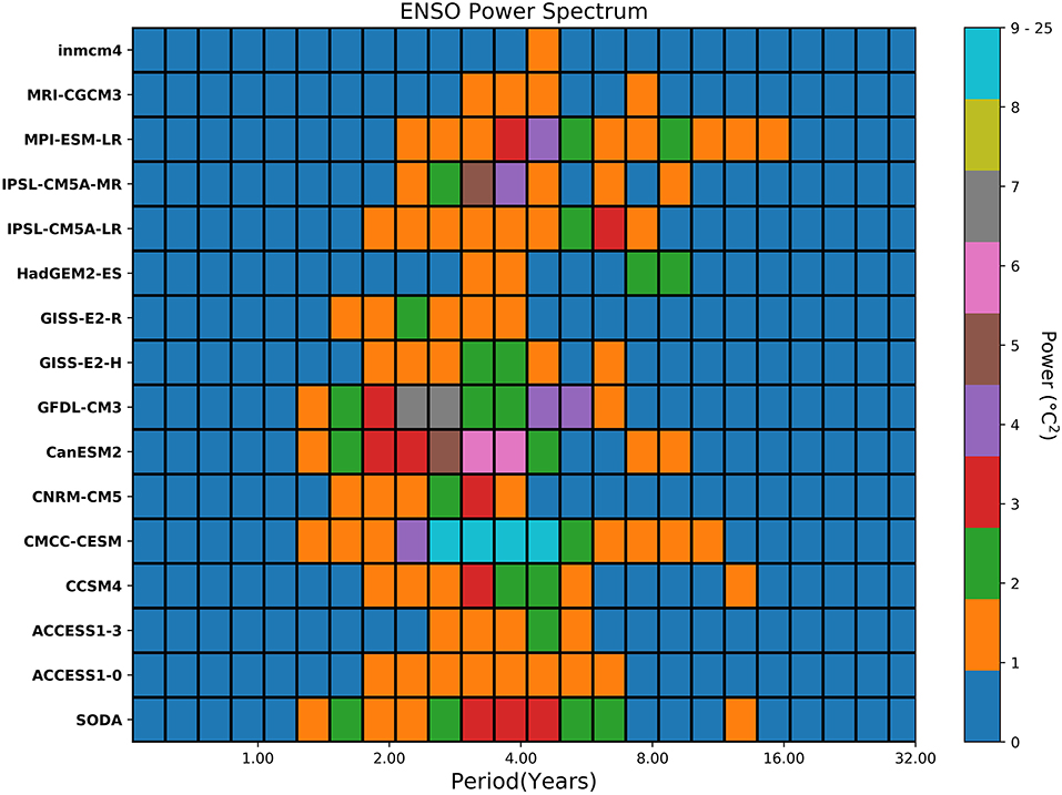
Figure 7. Power spectrum of Niño3.4 index during 1967–2005 for models and during 1980–2018 for SODA reanalysis. The period (in years) is on the x-axis and the power is shaded.

In Figure 8 we show the variance of the Niño-3.4 and IOD indices across the four seasons. In many models, the variances of the two indices are comparable in magnitude, while being characterized by an approximately 3:1 ratio in the observational dataset. Additionally, the Niño-3.4 -IOD cross-correlation (Supplementary Figure 3), which is linked to the directionality of the connections between the two modes and therefore the predictability potential across the basins, indicates that the Niño-3.4 variability lags, or co-occurs with, the IOD one in most models, while it leads by 2 months in the reanalysis. CNRM-CM5 emerges again as the model with the closest representation to the reanalysis. Cross-correlations between the Nino3.4 index and the SETIO and WTIO indices separately point to the eastern region of the IO as source of the bias (not shown).

FIGURE 8

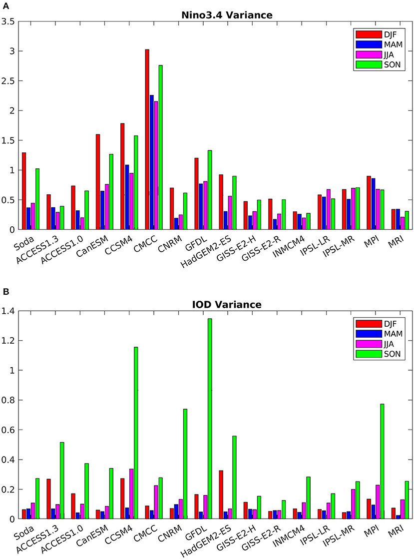
Figure 8. Seasonal variance of Niño3.4 (A) and IOD (B) indices during 1967–2005 for models and during 1980–2018 for SODA reanalysis.

To better highlight what limits the reliability of model climate predictions in the IO, we next examine briefly atmospheric and oceanic connections induced by developing ENSO events affect the IO and vice versa. We use standard correlation and regression analysis and our investigation does not aim at being exhaustive, but simply identifies possible biases that are shared among many models and appear to influence how predictability is simulated.

Atmospheric Teleconnection

The sea level pressure anomalies (SLPAs) over the SETIO region can be used as a proxy for the strength of atmospheric changes to the Walker circulation induced by ENSO over this area. A simple cross-correlation analysis shows that the modeled SLPa-ENSO relationship is captured by all models (Figure 9). The same is verified for the WTIO region (not shown). Interestingly CNRM-CM5 underestimates the signal, which is better captured by the GISS runs, CanESM or GFDL.

FIGURE 9

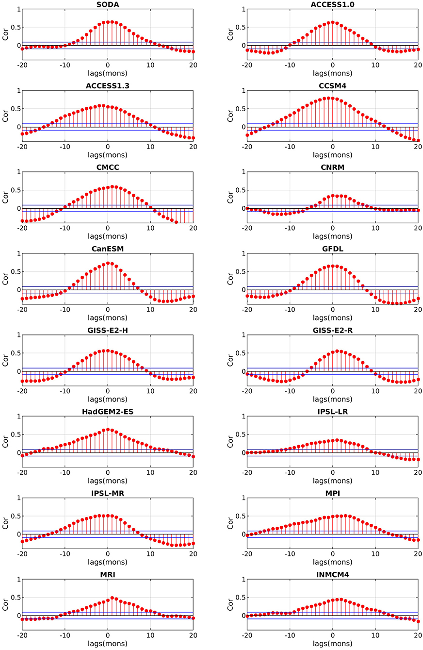
Figure 9. Cross correlation between the sea level pressure anomalies (SLPAs) over the SETIO region and the Niño3.4 Index during 1967–2005 for models and during 1980–2018 for SODA/ERA-interim reanalysis. Positive (negative) lags indicate SLPa lags (leads) the Niño3.4 Index.

From this simple analysis, we can infer that the bias in representing the IOD-ENSO interaction is not caused, at a first order, by a deficient representation of the atmospheric teleconnection from the Pacific into the IO. The IOD can independently modify the Walker circulation through air-sea interactions in SETIO (Izumo et al., 2010) but the ENSO influence on the Walker circulation is captured relatively well in all models. We will show later that the same cannot be said if we zoom onto the ITF region.

Oceanic Bridge

ENSO influences the IO ocean circulation by modulating the transport of warm and fresh water from the Pacific Warm Pool region into the IO via the ITF. Positive transport anomalies occur during La Niña events and vice versa in El Niño years (Meyers, 1996). England and Huang (2005) found the ITF transport, defined as the depth integrated transport over the whole water column at 8°S, 120°–131.5°E, to be anticorrelated with the Niño-3 index (SSTa averaged over 150°W−90°W, 5°S−5°N), with a maximum of −0.32 when the ITF lags ENSO by 9 months. Bracco et al. (2005) focused instead on the variability of the 20°C isotherm (Z20) that may more directly impact the upwelling in the SETIO region and found that that the fall correlation between the Z20 anomalies and Niño-3.4 reached −0.62 over the period 1958–2002.

In SODA, the maximum (minimum) transport occurs in boreal spring (fall), and the thermocline depth oscillates between 123 and 135 m. In the models, the annual cycle varies greatly in both amplitude and phase (Supplementary Figure 4). Several models have a thermocline that is 30 m or more too deep. Many, including INMCM4, GISS-E2- R, GISS-E2-H, MPI and CANESM, display an out of phase seasonal cycle (minimum in spring and maximum in fall) or shaped with two peaks. CMCC-CESM stands out for having a thermocline that is too shallow (about 20 m shallower than in the reanalysis in fall). CCSM, GFDL and IPSL-MR provide the closest representation to that in the reanalysis, with CCSM being the most realistic.

The cross-correlations between the Z20 anomalies averaged over the ITF region and Nino3.4 indices are shown in Figure 10. In the reanalysis, the maximum anticorrelation (−0.71) is found for the Niño-3.4 index lagging the ITF thermocline by 1 month. Statistically significant anticorrelations are found in all models but INMCM. However, the modeled anticorrelations are consistently maximized at about 3–5 months lags. The relationship between the Niño-3.4 index and the ITF is misrepresented by the models also when using the sea level difference between the western Pacific (WP; 0–10°N; 125°E−145°E) and the Eastern Indian Ocean (EIO; 10°S−20°S; 110°E−130°E) as ITF proxy (Mayer et al., 2018). Correlation coefficients are smaller than for Z20 but significant in the reanalyses, while the linkage is missed entirely in most models (Supplementary Figure 5). This is indicative of problems in the representation of both oceanic and atmospheric processes at the equator.

FIGURE 10

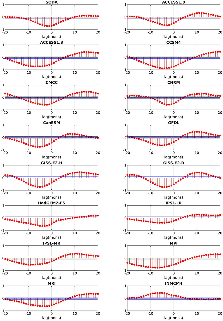
Figure 10. Cross correlation between the Indonesian Throughflow (ITF) thermocline depth anomaly and the Niño3.4 index during 1967–2005 for models and during 1980–2018 for SODA reanalysis. Positive (negative) lags indicate ITF lags (leads) the Niño3.4 index.

Finally, the regression maps of the SST over the tropics and of subsurface temperatures averages between 5°N and 5°S onto the IOD index are shown in Figures 11, 12. At the surface the link between the IOD and the ENSO anomalies are captured by most models but INMCM4 and underestimated by ACCESS1.3, HadGEM2-ES, followed by CCSM4, MPI and MRI and CNRM-CM5. At the ocean surbsurface, on the other hand, the regression patterns are generally strong underneath the warm pool, where they have the same sign of the SETIO region, but underestimated in the central and eastern Pacific. At the subsurface CNRM-CM5 emerges as closest to the reanalysis in the pattern representation. Modeled IODs somewhat mimic the characteristics of the unseasonal IOD events identified in the observations by Du et al. (2013), but for their seasonality. The unseasonal IOD are relevant in late spring and summer since the 1970's, and resemble the CMPI5 ones by being mostly independent of ENSO and forced by (too strong for fall in the CMIP5 case) equatorial winds. This figure also points to the differences in the representation of the ITF bathymetry among the models.

FIGURE 11

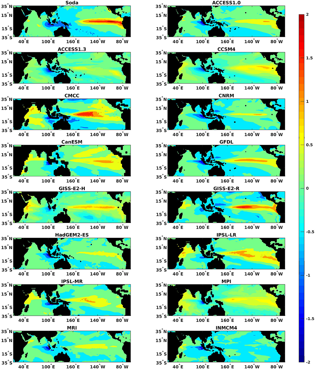
Figure 11. Regression maps of tropical Indo-Pacific sea surface temperatures on the IOD during the extended boreal fall season (ASON) of 1967–2005 for models and 1980–2018 for SODA reanalysis.

FIGURE 12

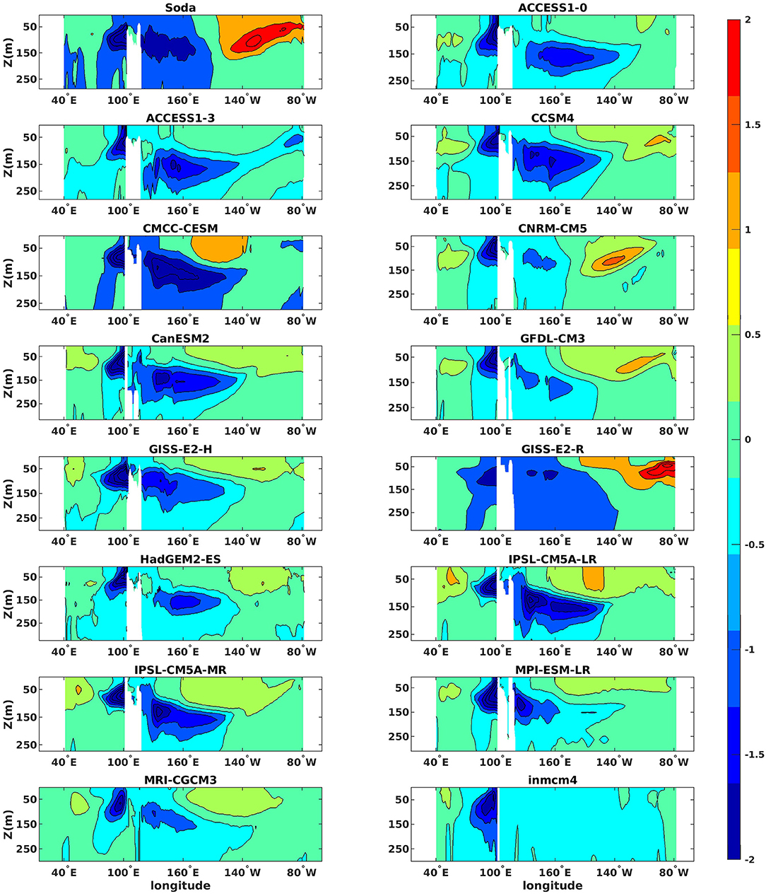
Figure 12. Regression maps of the tropical Indo-Pacific sea subsurface temperatures averaged between 5°N and 5°S onto the IOD during the extended boreal fall season (ASON) of 1967–2005 for models and 1980–2018 for SODA reanalysis.

The representation of the relative seasonal evolution of the two modes identified in the cross-correlations and the greater independence of the modeled IOD from the Pacific evolution emerge as problematic in all models. Our brief analysis extends the results by Cai and Cowan (2009) that highlighted other systematic biases in the IO and in particular (a) the western IO thermocline being deeper than the eastern IO while the opposite is verified in the observations so that the wave dynamics that transport the IOD temperature anomalies are not reproduced correctly; (b) slightly warmer SST in the western IO than eastern IO, while a much warmer eastern IO is observed; (c) stronger than observed climatological easterly winds over the equatorial Pacific.

Summary

Weather prediction is reliable to <10 days due to the atmosphere chaotic behavior, the sensitivity on the initial conditions and model limitations. Climate prediction, on the other hand, has the potential to extend to longer time scales due to the modulations exerted by its slowly varying component, the ocean. Climate modes that manifest as non-linear oscillations, such as the El Niño-Southern Oscillation, the Pacific Decadal Oscillation, the Atlantic Multi-Decadal Oscillation, the Indian Ocean Dipole, etc. further contribute to the extended range of potential predictability of the climate system.

Global warming is posed to modify these modes of natural variability that control much of the predictability at seasonal to interannual scales. Examples include the intensification of the IOD (Di Nezio et al., 2020), and a higher frequency of Central Pacific El Niños (Freund et al., 2019) observed in the last decade and projected to continue in the future, and shifts in its global-reaching teleconnections following the expansion of the Hadley cells (Kang and Lu, 2012). In light of the societal impacts that these modes exert by modulating surface temperatures, storm frequency, droughts and floods, their current and future predictability potential is of the uttermost importance. It remains, however, elusive due to the complexity of the climate system, the biases in climate models, the challenges implicit in quantifying it.

In this work, we introduced a new method, building upon tools developed within the non-linear dynamical systems community, to quantify predictability in terms of information entropy. The information entropy of a climate field quantifies the degree of complexity of a given region or grid point in terms of recurrence (how many times a phase space trajectory visits roughly the same area in the phase space over a given period) and evaluate how it varies over time. Given that the evolution of a climate field such as SST results from interactions of many fields, from atmospheric winds and heat fluxes to ocean currents, its space phase evolution accounts for all these interactions, linear and non-linear.

Most studies employing a comparable non-linear data analysis technique in climate science have focused on a limited number of 1-dimensional time series (i.e., paleoclimate proxies—one or few at the time—or their modeled equivalent) (Donges et al., 2011, 2015). The possibility to use it on large, multi-dimensional fields has been opened by Corso et al. (2018) by introducing a new entropy quantifier applicable to d-dimensional fields using the recurrent plot (RP) technique (Eckmann et al., 1987) without the need for embedding or phase space reconstruction. We applied it to the SST field in the tropical Pacific and Indian Ocean, comparing CMIP5 models and reanalysis data, over 39 years in the historical period and in the last 30 years of the XXI century RCP8.5 projections. We focused on the boreal fall season, when the ENSO signature is strong and the IOD has maximum variance in the Indian Ocean. Understanding the ENSO—IOD relation and the influence of the IOD on all countries facing the Indian Ocean is essential to improve prediction of extreme rainfall and droughts over Australia, India, Indonesia and East Africa. In these highly populated regions downscaled regional experiments (Hashizume et al., 2012) are limited by the representation of the large scale atmospheric and oceanic circulation.

Our analysis highlights the limitations that coupled climate models still face in addressing climate predictability and its potential changes. No robust signal is found in the models, in both basins, as to how predictability will evolve in the future when considering the projections for the last 30 years of the XXI century. In the historical period, very few models capture both pattern and intensity of the entropy signal of the reanalysis, and CNRM-CM5 outperforms all others in this regard. Interestingly, in an intercomparison performed using complex network analysis (Fountalis et al., 2015), CNRM-CM5 outperformed all other CMIP5 models also in the representation of rainfall patterns and their connectivities, but performed as well as several others in representing the (global) SST network. This again points to the power of the entropy quantifier as a measure of topological similarity linked to predictive power. The entropy quantifier, in summary, is a computationally efficient performance metric for coupled climate models, capable of capturing dynamical characteristics, both linear and non-linear, that goes beyond the climatology and local variability of the field under investigation, and delves into its topological properties.

We also showed that a biased representation of coupled equatorial dynamics and of the atmospheric and subsurface oceanic bridge between the Pacific and Indian Oceans via the ITF contributes to the poor representation of the Indo-Pacific entropy in fall. Incidentally, we verified that the intra-model variability is relatively small in the historical runs in the statistics presented, from the entropy to the cross-correlations, and each model behavior is consistent across ensemble members. Overall, many models struggle at the equator, in both basins, and display unrealistic regular dynamics in the IO, especially south of the equator and/or in the Arabian Sea.

Our results exemplify how information entropy may contribute a new powerful tool to investigate the potential predictability of the climate system. More work is needed to explore its relevance on time scales other than interannual, using higher or lower frequency time series as input to explore, for example, subseasonal phenomena o changes across millennia, and the entropy usefulness in analyzing fields other than SSTs. In the near future, we aim at applying it across time scales and with high frequency (at least daily) data to quantify how and where climate predictability emerges from the weather noise.

Data Availability Statement

Publicly available datasets were analyzed in this study. The SODA reanalysis data can be obtained from: https://www2.atmos.umd.edu/~ocean/index_files/soda3.4.2_mn_download_b.htm. ERA-Interim can be obtained from https://apps.ecmwf.int/datasets/data/interim-full-mnth/levtype=sfc/. Monthly mean output from Coupled Model Intercomparison Project Phase 5 (CMIP5) historical and RCP8.5 experiments are publicly available on https://esgf-node.llnl.gov/search/cmip5/. The entropy code can be found at https://github.com/FabriFalasca/NonLinear_TimeSeries_Analysis.

Author Contributions

OI performed all analyses. FF developed and optimized the software for the information entropy quantifier. AB coordinated the analyses and wrote the manuscript. All authors contributed to the interpretation of the results and approved the submitted version.

Funding

AB and FF were supported by the Department of Energy, Regional and Global Model Analysis (RGMA) Program, Grant No.: 0000253789.

Conflict of Interest

The authors declare that the research was conducted in the absence of any commercial or financial relationships that could be construed as a potential conflict of interest.

Acknowledgments

This research resulted from a term project during a course in the School of Earth and Atmospheric Sciences at Georgia Tech. We thank the School for contributing toward the publication costs of this work. We also thank the two reviewers who contributed to improving the original submission.

Supplementary Material

The Supplementary Material for this article can be found online at: https://www.frontiersin.org/articles/10.3389/fclim.2021.675840/full#supplementary-material

References

Allan, R., Chambers, D. P., Drosdowsky, W. L., Hendon, H. A. H., Latif, M. Z., Nicholls, N. S., et al. (2001). Is there an indian ocean dipole and is it independent of the el niño-southern oscillation. Clivar. Exch. 6, 18–22. doi: 10.5194/bg-10-6677-2013

PubMed Abstract | CrossRef Full Text | Google Scholar

Annamalai, H., Xie, S. P., McCreary, J. P., and Murtugudde, R. (2005). Impact of indian ocean sea surface temperature on developing el niño. J. Clim. 18, 302–319. doi: 10.1175/JCLI-3268.1

CrossRef Full Text | Google Scholar

Anyamba, A., Chretien, J.-P., Britch, S. C., Soebiyanto, R. P., Small, J. L., Jepsen, R., et al. (2019). Global disease outbreaks associated with the 2015–2016 El Niño event. Sci. Rep. 9:1930. doi: 10.1038/s41598-018-38034-z

PubMed Abstract | CrossRef Full Text | Google Scholar

Ashok, K., Guan, Z., and Yamagata, T. (2001). Impact of the indian ocean dipole on the relationship between the indian monsoon rainfall and enso. Geophys. Res. Lett. 28, 4499–4502. doi: 10.1029/2001GL013294

CrossRef Full Text | Google Scholar

Ashok, K., Guan, Z., and Yamagata, T. (2003). A look at the relationship between the enso and the indian ocean dipole. J. Meteorol. Soc. Japan 81, 41–56. doi: 10.2151/jmsj.81.41

CrossRef Full Text | Google Scholar

Balasis, G., Donner, R. V., Potirakis, S. M., Runge, J., Papadimitriou, C., Daglis, I. A., et al. (2013). Statistical mechanics and information-theoretic perspectives on complexity in the earth system. Entropy 15, 4844–4888. doi: 10.3390/e15114844

CrossRef Full Text | Google Scholar

Bandt, C., and Pompe, B. (2002). Permutation entropy: a natural complexity measure for time series. Phys. Rev. Lett. 88:174102. doi: 10.1103/PhysRevLett.88.174102

PubMed Abstract | CrossRef Full Text | Google Scholar

Behera, S. K., Krishnan, R., and Yamagata, T. (1999). Unusual ocean-atmosphere conditions in the tropical indian ocean during 1994. Geophys. Res. Lett. 26, 3001–3004. doi: 10.1029/1999GL010434

CrossRef Full Text | Google Scholar

Behera, S. K., Luo, J. J., Masson, S., Rao, S. A., Sakuma, H., and Yamagata, T. (2006). A CGCM study on the interaction between IOD and ENSO. J. Clim. 19, 1688–1705. doi: 10.1175/JCLI3797.1

CrossRef Full Text | Google Scholar

Bellenger, H., Guilyardi, E., Leloup, J., Lengaigne, M., and Vialard, J. (2014). ENSO representation in climate models: from CMIP3 to CMIP5. Clim. Dyn. 42, 1999–2018. doi: 10.1007/s00382-013-1783-z

CrossRef Full Text | Google Scholar

Bjerknes, J. (1966). A possible response of the atmospheric Hadley circulation to equatorial anomalies of ocean temperature. Tellus 18, 820–829. doi: 10.3402/tellusa.v18i4.9712

CrossRef Full Text | Google Scholar

Bjerknes, J. (1969). Atmospheric teleconnections from the equatorial Pacific. Monthly Weather Rev. 97, 163–172. doi: 10.1175/1520-0493(1969)097<0163:ATFTEP>2.3.CO;2

CrossRef Full Text | Google Scholar

Black, E., Slingo, J., and Sperber, K. R. (2003). An observational study of the relationship between excessively strong short rains in coastal East Africa and Indian Ocean sst. Mon. Wea. Rev. 131, 74–94. doi: 10.1175/1520-0493(2003)131<0074:AOSOTR>2.0.CO;2

CrossRef Full Text | Google Scholar

Bracco, A., Kucharski, F., Molteni, F., Hazeleger, W., and Severijns, C. (2005). Internal and forced modes of variability in the Indian Ocean. Geophys. Res. Lett. 32:L12707. doi: 10.1029/2005GL023154

CrossRef Full Text | Google Scholar

Cai, W., and Cowan, T. (2009). Why is the amplitude of the indian ocean dipole overly large in cmip3 and CMIP5 climate models? Geophys. Res. Lett. 40, 1200–1205. doi: 10.1002/grl.50208

CrossRef Full Text | Google Scholar

Cai, W., Hendon, H. H., and Meyers, G. (2005). Indian ocean dipolelike variability in the csiro mark 3 coupled climate model. J. Clim. 18, 1449–1468. doi: 10.1175/JCLI3332.1

CrossRef Full Text | Google Scholar

Cai, W., Pan, A., Roemmich, D., Cowan, T., and Guo, X. (2009). Argo proles a rare occurrence of three consecutive positive indian ocean dipole events, 2006–2008. Geophys. Res. Lett. 36. doi: 10.1029/2008GL037038

CrossRef Full Text | Google Scholar

Cai, W., Santoso, A., Wang, G., Yeh, S.-W., An, S.-I., Cobb, K. M., et al. (2015). ENSO and greenhouse warming. Nat. Clim. Change 5, 849–859. doi: 10.1038/nclimate2743

CrossRef Full Text | Google Scholar

Carton, J. A., Chepurin, G. A., and Chen, L. (2018). Soda3: a new ocean climate reanalysis. J. Clim. 31, 6967–6983. doi: 10.1175/JCLI-D-18-0149.1

CrossRef Full Text | Google Scholar

Chen, C., Cane, M., Wittenberg, A., and Chen, D. (2017). ENSO in the CMIP5 simulations: life cycles, diversity, and responses to climate change. J. Clim. 30, 775–801. doi: 10.1175/JCLI-D-15-0901.1

CrossRef Full Text | Google Scholar

Corso, G., Prado, T., Lima, G., Kurths, J., and Lopes, S. (2018). Quantifying entropy using recurrence matrix microstates. Chaos 28:083108. doi: 10.1063/1.5042026

PubMed Abstract | CrossRef Full Text | Google Scholar

Cvitanović, P., Artuso, R., Mainieri, R., Tanner, G., and Vattay, G. (2016). Chaos: Classical and Quantum, ChaosBook.org. Copenhagen: Niels Bohr Institute.

Dee, D. P., Uppala, S. M., Simmons, A. J., Berrisford, P., Poli, P., Kobayashi, S., et al. (2011). The ERA-Interim reanalysis: configuration and performance of the data assimilation system. Q. J. R. Meteorol. Soc. 137, 553–597. doi: 10.1002/qj.828

CrossRef Full Text | Google Scholar

Dhiman, R. C., and Sarkar, S. (2017). El Niño southern oscillation as an early warning tool for malaria outbreaks in India. Malaria J. 16:122. doi: 10.1186/s12936-017-1779-y

PubMed Abstract | CrossRef Full Text | Google Scholar

Di Nezio, P., Puy, M., Thirumalai, K., Jin, F. F., and Tierney, J. (2020). Emergence of an equatorial mode of climate variability in the Indian Ocean. Sci. Adv. 6:7684. doi: 10.1126/sciadv.aay7684

PubMed Abstract | CrossRef Full Text | Google Scholar

Donges, J. F., Donner, R. V., Marwan, N., Breitenbach, S. F. M., Rehfeld, K., and Kurths, J. (2015). Non-linear regime shifts in Holocene Asian monsoon variability: potential impacts on cultural change and migratory patterns. Clim. Past 11, 709–741. doi: 10.5194/cp-11-709-2015

CrossRef Full Text | Google Scholar

Donges, J. F., Donner, R. V., Trauth, M. H., Marwan, N., Schellnhuber, H. J., and Kurths, J. (2011). Nonlinear detection of paleoclimate-variability transitions possibly related to human evolution. Proc. Natl. Acad. Sci. U.S.A. 108, 20422–20427. doi: 10.1073/pnas.1117052108

PubMed Abstract | CrossRef Full Text | Google Scholar

Donner, R., Small, M., Donges, J., Marwan, N., Zou, Y., Xiang, R., et al. (2011). Recurrence-based time series analysis by means of complex network methods. Int. J. Bifurcat. Chaos 21, 1019–1046. doi: 10.1142/S0218127411029021

PubMed Abstract | CrossRef Full Text | Google Scholar

Du, Y., Cai, W., and Wu, Y. (2013). A new type of the Indian Ocean dipole since the Mid-1970s. J. Clim. 26, 959–972. doi: 10.1175/JCLI-D-12-00047.1

CrossRef Full Text | Google Scholar

Duan, W., and Wei, C. (2013). The ‘spring predictability barrier’ for ENSO predictions and its possible mechanism: results from a fully coupled model. Int. J. Climatol. 33, 1280–1292. doi: 10.1002/joc.3513

CrossRef Full Text | Google Scholar

Eckmann, J.-P., Kamphorst, S. O., and Ruelle, D. (1987). Recurrence plots of dynamical systems. Europhys. Lett. 5, 973–977. doi: 10.1209/0295-5075/4/9/004

CrossRef Full Text | Google Scholar

England, M. H., and Huang, F. (2005). On the interannual variability of the Indonesian throughflow and its linkage with ENSO. J. Clim. 18, 1435–1444. doi: 10.1175/JCLI3322.1

CrossRef Full Text | Google Scholar

Falasca, F., Crétat, J., Braconnot, P., and Bracco, A. (2020). Spatiotemporal complexity and time-dependent networks in sea surface temperature from mid- to late Holocene. Eur. Phys. J. Plus 135:392. doi: 10.1140/epjp/s13360-020-00403-x

CrossRef Full Text | Google Scholar

Fountalis, I., Bracco, A., and Dovrolis, C. (2015). ENSO in CMIP5 simulations: network connectivity from the recent past to the twenty-third century. Clim. Dyn. 45, 511–538. doi: 10.1007/s00382-014-2412-1

CrossRef Full Text | Google Scholar

Freund, M. B., Henley, B. J., Karoly, D. J., McGregor, H. V., Abram, N. J., and Dommenget, D. (2019). Higher frequency of central Pacific El Niño events in recent decades relative to past centuries. Nat. Geosci. 12, 450–455. doi: 10.1038/s41561-019-0353-3

CrossRef Full Text | Google Scholar

Garland, J., Jones, T. R., Neuder, M., White, J. W. C., and Bradley, E. (2019). An information-theoretic approach to extracting climate signals from deep polar ice cores. Chaos 29:101105. doi: 10.1063/1.5127211

PubMed Abstract | CrossRef Full Text | Google Scholar

Gilpin, W. (2020). Deep Reconstruction of Strange Attractors From Time Series. Cambridge, MA: Harvard University.

Google Scholar

Gualdi, S., Guilyardi, E., Navarra, A., Masina, S., and Delecluse, P. (2003). The interannual variability in the tropical Indian Ocean as simulated by a CGCM. Clim. Dyn. 20, 567–582. doi: 10.1007/s00382-002-0295-z

CrossRef Full Text | Google Scholar

Guan, Z., Ashok, K., and Yamagata, T. (2003). Summertime response of the tropical atmosphere to the Indian Ocean Dipole sea surface temperature anomalies. J. Meteorol. Society of Japan. Ser. II 81, 533–561. doi: 10.2151/jmsj.81.533

CrossRef Full Text | Google Scholar

Hashizume, M., Chaves, L. F., and Minakawa, N. (2012). Indian Ocean Dipole drives malaria resurgence in east african highlands. Sci. Rep. 2:269. doi: 10.1038/srep00269

PubMed Abstract | CrossRef Full Text | Google Scholar

IPCC (2014). Climate Change 2014: Synthesis Report. Contribution of Working Groups I, II and III to the Fifth Assessment Report of the Intergovernmental Panel on Climate Change. Technical report, IPCC, Geneva, Switzerland.

Google Scholar

Izumo, T., Vialard, J., Lengaigne, M., de Boyer Montegut, C., Behera, S. K., Luo, J.-J., et al. (2010). Influence of the state of the Indian Ocean Dipole on the following year's El Niño. Nat. Geosci. 3:168. doi: 10.1038/ngeo760

CrossRef Full Text | Google Scholar

Kajtar, J. B., Santoso, A., and England, M. H. W. (2015). Indo-pacific climate interactions in the absence of an indonesian throughflow. J. Clim. 28, 5017–5029. doi: 10.1175/JCLI-D-14-00114.1

CrossRef Full Text | Google Scholar

Kang, S. M., and Lu, J. (2012). Expansion of the Hadley cell under global warming: winter versus summer. J. Clim. 25, 8387–8393. doi: 10.1175/JCLI-D-12-00323.1

CrossRef Full Text | Google Scholar

Koebbe, M., and Mayer-Kress, G. (1992). “Use of recurrence plots in the analysis of time-series data,” in Nonlinear Modeling and Forecasting, eds M. Casdagli and S. Eubank (New York, NY: Addison Wesley).

Google Scholar

Kovats, R. S. (2000). El Niño and human health. Bull World Health Organ., 78, 1127–1135. Available online at: https://www.ncbi.nlm.nih.gov/pmc/articles/PMC2560836/pdf/11019461.pdf

Google Scholar

Kreppel, K., Caminade, C., Govella, N., Morse, A. P., Ferguson, H. M., and Baylis, M. (2019). Impact of ENSO 2016–17 on regional climate and malaria vector dynamics in tanzania. Environ. Res. Lett. 14:075009.075014 doi: 10.1088/1748-9326/ab26c7

CrossRef Full Text | Google Scholar

Kug, J., Li, T., An, S.-I., Kang, I., Luo, J., Masson, S., et al. (2006). Role of the ensoindian ocean coupling on enso variability in a coupled gcm. Geophys. Res. Lett. 33:24916. doi: 10.1029/2005GL024916

CrossRef Full Text | Google Scholar

Lau, N.-C., Leetmaa, A., Nath, M. J., and Wang, H.-L. (2005). Influences of ENSO-induced Indo–western Pacific SST anomalies on extratropical atmospheric variability during the boreal summer. J. Clim. 18, 2922–2942. doi: 10.1175/JCLI3445.1

CrossRef Full Text | Google Scholar

Lau, N.-C., and Nath, M. J. (2003). Atmosphere–ocean variations in the Indo-Oacific sector during ENSO episodes. J. Clim. 16, 3–20. doi: 10.1175/1520-0442(2003)016<0003:AOVITI>2.0.CO;2

CrossRef Full Text | Google Scholar

Li, C., and Mu, C. (2001). The influence of the Indian Ocean Dipole on atmospheric circulation and climate. Adv. Atmosphere. Sci. 18, 831–843. doi: 10.1007/BF03403506

CrossRef Full Text | Google Scholar

Lorenz, E. N. (1963). Deterministic nonperiodic flow. J. Atmosphere. Sci. 20, 130–141. doi: 10.1175/1520-0469(1963)020<0130:DNF>2.0.CO;2

CrossRef Full Text | Google Scholar

Manneville, P. (1990). “Characterization of temporal chaos,” in Dissipative Structures and Weak Turbulence, ed P. Manneville (Boston, MA: Academic Press). doi: 10.1016/B978-0-08-092445-8.50011-0

CrossRef Full Text

Marwan, N. (2011). How to avoid potential pitfalls in recurrence plot based data analysis. Int. J. Bifurcat. Chaos 21, 1003–1017. doi: 10.1142/S0218127411029008

CrossRef Full Text | Google Scholar

Marwan, N., Romano, M. C., Thiel, M., and Kurths, J. (2007). Recurrence plots for the analysis of complex systems. Phys. Rep. 438, 237–329. doi: 10.1016/j.physrep.2006.11.001

CrossRef Full Text

May, R. M. (1976). Simple mathematical models with very complicated dynamics. Nature 261, 459–467. doi: 10.1038/261459a0

PubMed Abstract | CrossRef Full Text | Google Scholar

Mayer, M., Alonso Balmaseda, M., and Haimberger, L. (2018). Unprecedented 2015/2016 Indopacific heat transfer speeds up tropical pacific heat recharge. Geophys. Res. Lett. 45, 3274–3284. doi: 10.1002/2018GL077106

PubMed Abstract | CrossRef Full Text | Google Scholar

Meyers, G. (1996). Variation of Indonesian throughflow and the El Niño-Southern oscillation. J. Geophys. Res. Oceans 101, 12255–12263. doi: 10.1029/95JC03729

CrossRef Full Text | Google Scholar

Mindlin, G. M., and Gilmore, R. (1992). Topological analysis and synthesis of chaotic time series. Phys. D Nonlinear Phenomena 58, 229–242. doi: 10.1016/0167-2789(92)90111-Y

CrossRef Full Text | Google Scholar

Poincaré, P. (1890). Sur le probleme des trois corps et les équations de la dynamique. Acta Mathe. 13, 1–271. doi: 10.1007/BF02392514

CrossRef Full Text

Prado, T., Corso, G., Santos Lima, G., Budzinski, R., Boaretto, B., Ferrari, F., et al. (2020). Maximum entropy principle in recurrence plot analysis on stochastic and chaotic systems. Chaos 30:043123. doi: 10.1063/1.5125921

PubMed Abstract | CrossRef Full Text | Google Scholar

Riedl, N. (2013). Practical considerations of permutation entropy. Eur. Phys. J. Spec. Topics 222, 249–262. doi: 10.1140/epjst/e2013-01862-7

CrossRef Full Text | Google Scholar

Saco, P. M., Carpi, L. C., Figliola, A., Serrano, E., and Rosso, O. A. (2010). Entropy analysis of the dynamics of El Niño/Southern oscillation during the holocene. Phys. A: Statist. Mech. Appl. 389, 5022–5027. doi: 10.1016/j.physa.2010.07.006

CrossRef Full Text | Google Scholar

Saji, N. H., Goswami, B. N., Vinayachandran, P. N., and Yamagata, T. (1999). A dipole mode in the tropical indian ocean. Nature 401, 360–363. doi: 10.1038/43854

PubMed Abstract | CrossRef Full Text | Google Scholar

Saji, N. H., and Yamagata, T. (2003). Possible impacts of Indian Ocean Dipole mode events on global climate. Clim. Res. 25, 151–169. doi: 10.3354/cr025151

CrossRef Full Text | Google Scholar

Santoso, A. W, England, M. H., and Phipps, S. J. (2011). The role of the Indonesian throughflow on ENSO dynamics in a coupled climate model. J. Clim. 24, 585–601. doi: 10.1175/2010JCLI3745.1

CrossRef Full Text | Google Scholar

Shi, W. (2007). “Lyapunov exponent analysis to chaotic phenomena of marine power system,” in Fault Detection, Supervision and Safety of Technical Processes 2006, ed H. Y. Zhang (Oxford: Elsevier Science Ltd.). doi: 10.1016/B978-008044485-7/50251-7

CrossRef Full Text | Google Scholar

Song, Q., Vecchi, G. A., and Rosati, A. J. (2007). The role of the Indonesian throughflow in the Indo–Pacific climate variability in the GFDL coupled climate model. J. Clim. 20, 2434–2451. doi: 10.1175/JCLI4133.1

CrossRef Full Text | Google Scholar

Sprintall, J., Chong, J., Syamsudin, F., Morawitz, W., Hautala, S., Bray, N., et al. (1999). Dynamics of the south Java current in the Indo-Australian basin. Geophys. Res. Lett. 26, 2493–2496. doi: 10.1029/1999GL002320

CrossRef Full Text | Google Scholar

Takens, F. (1981). “Detecting strange attractors in fluid turbulence,” in Dynamical System and Turbulence, Lecture Notes in Mathematics, eds D. A. Rand and L. S. Young (Berlin: Springer Verlag). doi: 10.1007/BFb0091924

CrossRef Full Text | Google Scholar

Taylor, K. E., Stouffer, R. J., and Meehl, G. A. (2012). An overview of CMIP5 and the experiment design. Bull. Am. Meteorol. Soc. 93, 485–498. doi: 10.1175/BAMS-D-11-00094.1

CrossRef Full Text | Google Scholar

Torrence, C., and Webster, P. J. (1998). The annual cycle of persistence in the El Niño-Southern oscillation. Q. J. R. Meteorol. Soc. 124, 1985–2004. doi: 10.1256/smsqj.55009

CrossRef Full Text | Google Scholar

van Sebille, E., Sprintall, J., Schwarzkopf, F. U., Sen Gupta, A., Santoso, A., England, M. H., et al. (2014). Pacific-to-indian ocean connectivity: Tasman leakage, Indonesian Throughflow, and the role of ENSO. J. Geophys. Res. Oceans 119, 1365–1382. doi: 10.1002/2013JC009525

CrossRef Full Text | Google Scholar

Wajsowicz, R. C., and Schneider, E. K. (2001). The Indonesian Throughflow's effect on global climate determined from the cola coupled climate system. J. Clim. 14, 3029–3042. doi: 10.1175/1520-0442(2001)014<3029:TITSEO>2.0.CO;2

CrossRef Full Text | Google Scholar

Webber, C., and Marwan, N., (eds.). (2015). Recurrence Quantification Analysis. Understanding Complex Systems. Cham: Springer. doi: 10.1007/978-3-319-07155-8

CrossRef Full Text | Google Scholar

Webster, P. J., Moore, A. M., Loschnigg, J. P., and Leben, R. R. (1999). Coupled ocean-atmosphere dynamics in the Indian Ocean during 1997-98. Nature 401, 356–360. doi: 10.1038/43848

PubMed Abstract | CrossRef Full Text | Google Scholar

Weller, E., and Cai, W. (2013). Realism of the Indian Ocean Dipole in CMIP5 models: the implications for climate projections. J. Clim. 26, 6649–6659. doi: 10.1175/JCLI-D-12-00807.1

CrossRef Full Text | Google Scholar

Yeh, S.-W., Cai, W., Min, S.-K., McPhaden, M. J., Dommenget, D., Dewitte, B., et al. (2018). ENSO atmospheric teleconnections and their response to greenhouse gas forcing. Rev. Geophys. 56, 185–206. doi: 10.1002/2017RG000568

CrossRef Full Text | Google Scholar

Yuan, D., Wang, J., Xu, T., Xu, P., Hui, Z., Zhao, X., et al. (2011). Forcing of the Indian Ocean Dipole on the interannual variations of the tropical Pacific Ocean: roles of the Indonesian Throughflow. J. Clim. 24, 3593–3608. doi: 10.1175/2011JCLI3649.1

CrossRef Full Text | Google Scholar

Zbilut, J. P., and Webber, C. L. (1992). Embeddings and delays as derived quantification of recurrence plots. Phys. Lett. A 171, 199–203. doi: 10.1016/0375-9601(92)90426-M

CrossRef Full Text | Google Scholar

Zbilut, J. P., Zaldivar-Comenges, J. M., and Strozzi, F. (2002). Recurrence quantification based Liapunov exponents for monitoring divergence in experimental data. Phys. Lett. A 297, 173–181. doi: 10.1016/S0375-9601(02)00436-X

CrossRef Full Text | Google Scholar

Zhou, Q., Duan, W., Mu, M., and Feng, R. (2015). Influence of positive and negative indian ocean dipoles on ENSO via the Indonesian Throughflow: results from sensitivity experiments. Adv. Atmosphere. Sci. 32, 783–793. doi: 10.1007/s00376-014-4141-0

CrossRef Full Text | Google Scholar

Zuo, H., Balmaseda, M. A., Tietsche, S., Mogensen, K., and Mayer, M. (2019). The ecmwf operational ensemble reanalysis analysis system for ocean and sea ice: a description of the system and assessment. Ocean Sci. 15, 779–808. doi: 10.5194/os-15-779-2019

CrossRef Full Text | Google Scholar