 Hendrik Großelindemann
 Svenja Ryan
 Caroline C. Ummenhofer
 Torge Martin
 Arne Biastoch1,2
- 1GEOMAR Helmholtz Centre for Ocean Research Kiel, Kiel, Germany
- 2Christian-Albrechts Universität zu Kiel, Kiel, Germany
- 3Woods Hole Oceanographic Institution, Woods Hole, MA, United States
Marine Heatwaves (MHWs) are ocean extreme events, characterized by anomalously high temperatures, which can have significant ecological impacts. The Northeast U.S. continental shelf is of great economical importance as it is home to a highly productive ecosystem. Local warming rates exceed the global average and the region experienced multiple MHWs in the last decade with severe consequences for regional fisheries. Due to the lack of subsurface observations, the depth-extent of MHWs is not well-known, which hampers the assessment of impacts on pelagic and benthic ecosystems. This study utilizes a global ocean circulation model with a high-resolution (1/20°) nest in the Atlantic to investigate the depth structure of MHWs and associated drivers on the Northeast U.S. continental shelf. It is shown that MHWs exhibit varying spatial extents, with some only occurring at depth. The highest intensities are found around 100 m depth with temperatures exceeding the climatological mean by up to 7°C, while surface intensities are typically smaller (around 3°C). Distinct vertical structures are associated with different spatial MHW patterns and drivers. Investigation of the co-variability of temperature and salinity reveals that over 80% of MHWs at depth (>50 m) coincide with extreme salinity anomalies. Two case studies provide insight into opposing MHW patterns at the surface and at depth, being forced by anomalous air-sea heat fluxes and Gulf Stream warm core ring interaction, respectively. The results highlight the importance of local ocean dynamics and the need to realistically represent them in climate models.
1. Introduction
Marine Heatwaves (MHWs) are characterized by extreme ocean temperatures, defined as discrete, prolonged and anomalously warm events (Hobday et al., 2016). MHWs can have extensive impacts on marine ecosystems and ultimately socio-economics, by causing mass mortality of marine species and even sea-birds (Mills et al., 2013; Short et al., 2015; Jones et al., 2018) or species redistribution (Smale et al., 2019; Wernberg, 2020), which can influence fisheries and local economics (Mills et al., 2013). These impacts are likely to become worse with ongoing global warming: an increase of MHW frequency (34%) and duration (17%) over the last century (1925–2016) was shown (Oliver et al., 2018, 2021), a trend that is projected to continue during the twenty-first century (Oliver et al., 2019). In order to improve our predictive skills and adaptation management, it is crucial to understand the physical characteristics and drivers of MHWs, as well as their potential impacts.
The Northwest Atlantic, in particular the Northeast U.S. continental shelf, is among the fastest warming regions in the world (Figure 1; Wu et al., 2012; Forsyth et al., 2015; Saba et al., 2016). This exposes the region to an increased risk of occurrence of MHWs and accumulative thermal stress on the marine ecosystem. MHWs in the recent decade have already provided us with a taste of their impacts, even leading to international tensions as observed in 2012, when a record MHW in spring lead to early and intense landings of American lobster (Homarus americanus), causing an oversupply on the market and a breakdown of the supply chain (Mills et al., 2013). Lobster is the region's highest value fishery, however other fisheries were also impacted such as Atlantic Cod (Gardus morhua), longfin squid [Doryteuthis (Amerigo) pealeii] and blue crabs (Callinectes sapidus), in particular in the Gulf of Main (Mills et al., 2013; Pershing et al., 2015, 2018). After another strong MHW in 2016 (Perez et al., 2021) that lead to similar landings, there is evidence that the lobster industry was able to make successful adaptions to the supply chain based on their previous experience (Pershing et al., 2018).
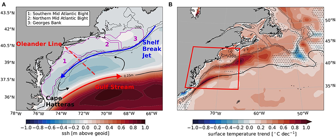
Figure 1. Map of the study region and observed surface temperature trends; (A) Magenta contours indicate shelf ecoboxes defined by Chen et al. (2020); red dashed line indicates mean track of the CMV Oleander; shaded is the mean absolute dynamic topography from CMEMS altimeter data for 1993 to 2019 with the 0.25 m level indicated by the black line; red arrow indicates the Gulf Stream, blue the Shelfbreak Jet and black the recirculation gyre; (B) linearly regressed surface temperature trends from NOAA OISST annual values for 1982–2019; stippling indicates non-significant values below the 99% level; red box marks region of (A); 0.25 m absolute dynamic topography contour is shown for reference; dashed black lines in (A,B) show isobaths of 200, 1,000, 2,000, and 4,000 m depth.
It has been shown that globally the mean increase in temperatures drives MHW trends, however in western boundary regions, changes in variance also plays an important role due to highly complex ocean dynamics (Oliver et al., 2021). The warm and salty Gulf Stream flows poleward as the western boundary current of the North Atlantic subtropical gyre (Figure 1). After separating at Cape Hatteras at approximately 30°N, the Gulf Stream turns into a free flowing current and begins to meander, which leads to the formation of Warm Core Rings (WCRs) along its northern edge. WCRs are anticyclonic mesoscale eddies that propagate westward toward the U.S. coast and the adjacent continental shelf, advecting warm and salty waters into this region (Fratantoni and Pickart, 2007). This process leads to interactions with the cooler and fresher shelf waters as well as mid-depth salinity intrusions onto the shelf (Gawarkiewicz et al., 2018). A significant regime shift to a higher WCR formation rate occurred around 2000 (Gangopadhyay et al., 2019), along with a recent westward movement of the Gulf Stream destabilization point (Andres, 2016). This denotes that the Gulf Stream starts meandering further west which leads to increased open-ocean/shelf interaction.
The Shelfbreak Jet flows equatorward above the shelfbreak as an extension of the Labrador Current, transporting cooler and fresher water from the Labrador Sea toward Cape Hatteras (Flagg et al., 2006; Fratantoni and Pickart, 2007; Gawarkiewicz et al., 2008; Forsyth et al., 2020; New et al., 2021). The boundary between cold and fresh shelf waters and warm and salty offshore waters in the Slope Sea denotes the Shelfbreak Front (Gawarkiewicz et al., 2018). The Shelfbreak Jet and associated front can act as a dynamical barrier between the two water masses. However, mid-depth and bottom intrusions can occur due to, for example, density compensating effects of temperature and salinity or the formation of local pressure gradients that drive on-shore geostrophic flow (Lentz, 2003; Gawarkiewicz et al., 2018; Chen et al., 2022). A cyclonic recirculation gyre is maintained by the westward flowing water over the continental slope and the eastward flowing warm water in the Slope Sea and the Gulf Stream (see Figure 1; Csanady and Hamilton, 1988; Andres et al., 2020). The mixture of the northern and southern source waters in the Slope Sea is referred to as slope water (Csanady and Hamilton, 1988). Its composition, i.e., fractions of source water masses, is impacted by changes in the large-scale circulation such as latitudinal shifts of the Gulf Stream (Neto et al., 2021). The complexity of the region's circulation system poses a challenge for understanding the large observed and projected warming trends and associated increase in extreme events in the region.
MHW formation can occur as an effect of atmosphere-ocean interactions as well as of advective processes (Oliver et al., 2021). It has been shown that the record MHW in this region in 2012 was primarily driven by atmospheric jet stream variability in 2012, where an anomalously northward position lead to an increased heatflux into the ocean (Chen et al., 2014a, 2015). On the other hand in 2017, in-situ observations revealed an advective MHW, which was initiated by cross-shelf advection in the presence of a WCR, with temperature anomalies up to 6°C (Gawarkiewicz et al., 2019; Chen et al., 2022). Furthermore, Perez et al. (2021) showed that both processes play an important role for the spatio-temporal sea surface temperature (SST) patterns associated with MHWs on the Northwest Atlantic continental shelf and slope. Most MHW studies have focused on SST due to the lack of continuous subsurface observations. However, recent studies investigated the depth extent of MHWs and associated drivers; in coastal waters off eastern Australia MHWs were observed using mooring data, spanning across 100 m depth, driven by downwelling favorable winds (Schaeffer and Roughan, 2017). Argo data revealed that MHWs in the region can occur down to a depth of 1,000 m withoug having a surface expression, driven by mesoscale eddies spinning off the East Australian Current, the local western boundary current (Elzahaby and Schaeffer, 2019). Ryan et al. (2021) used a global ocean model to investigate the depth structure of Ningaloo Niño and Niña events off Western Australia and found that temperature anomalies extended to a depth of 300 m or more and have a seasonally dependent subsurface peak driven by thermocline variability, which in turn is associated with seasonally reversing Monsoon winds that generate a downwelling coastal wave. Similarly, Hu et al. (2021) observed seasonally dependent subsurface MHWs in the upper thermocline layer in the western Pacific driven by anomalous Ekman downwelling. While many MHW studies have a global scope, these examples show that understanding the respective regional ocean circulation and variability is a key to investigate MHW drivers, in particular for subsurface events.
The current study utilizes a high resolution (1/20° nest), eddy-resolving global ocean model to investigate the depth structure of MHWs on the southern northeast U.S. continental shelf, comprising Georges Bank and the Middle Atlantic Bight (Figure 1). The model's skill in resolving the regional circulation is investigated for two simulations with different resolutions, one eddy-permitting (1/4°) and one eddy-resolving (nest of 1/20°) (Section 3.1). The hydrography of the shelf region in the eddy-resolving simulation is briefly described (Section 3.2). MHW events are detected throughout the whole water column and then examined for their depth structure (Section 3.3). MHW metrics (duration and intensities), are analyzed across depth and salinity extremes are detected as well to investigate connected processes and potential drivers followed by the seasonal distribution of MHW metrics (Section 3.4). Finally, two case studies of different types of MHWs are presented for a more detailed investigation regarding the depth structures of temperature and salinity anomalies as well as their spatio-temporal distribution (Section 3.5) followed by a discussion (Section 4).
2. Data and Methods
2.1. Model Description
This study analyzes two hindcast simulations from the NEMO (Nucleus for European Modeling of the Ocean, v3.6, Madec, 2016) ocean and sea-ice model, performed by GEOMAR, Helmholtz Center for Ocean Research Kiel, Germany. It runs on a global tripolar ORCA025 grid with an eddy-permitting horizontal resolution of 1/4° and 46 geopotential z-levels of varying thickness from 6 m at the surface to 250 m at depth. Bottom topography is interpolated from 1-min Gridded Global Relief Data ETOPO1 (Amante and Eakins, 2009) and represented by partial steps (Barnier et al., 2006). The ocean model is coupled to the Louvain-la-Neuve Sea Ice Model version 2 (LIM2-VP; Fichefet and Maqueda, 1997). The model is forced at the surface by the JRA55-do (v1.4) dataset, which is an atmospheric reanalysis product based on the full observing system starting in 1958 until present. It includes components for wind, thermal and haline forcings (the latter including river runoff), with adjustments to match observational datasets (Kobayashi et al., 2015; Tsujino et al., 2018). The data are applied through Bulk formulae from Large and Yeager (2009) to calculate fluxes and wind stress. Initialization is performed from a state of rest with the Levitus World Ocean Atlas (WOA; Levitus et al., 1998) with modifications in the polar regions from PHC (Polar Science Center Hydrographic Climatology), which represents a global ocean hydrography with a high-quality Arctic Ocean (Steele et al., 2001). A relaxation of sea surface salinity (SSS) toward observed climatological conditions from WOA is applied, a method commonly required in global ocean models to prevent spurious model drift (Griffies et al., 2009). Here, a piston velocity of 50 m per year (corresponding to a damping timescale of 44 days for the 6-m surface level) was used. A set of two model simulations is used and described briefly below. More details on the model set up and performance can be found in Biastoch et al. (2021).
2.1.1. ORCA025 and VIKINGX20
The global ORCA025 simulation serves as a standalone model and reference case to demonstrate the importance of explicitly resolving mesoscale dynamics in the region of interest. The latter is achieved by embedding a regional high-resolution (1/20°) nest, VIKING20X, covering the Atlantic from 33.5°S to 65°N. Two-way nesting ensures live updates between global host and nest models during runtime. The nest receives boundary conditions from the lower resolution global host model, while the latter receives updates from the nested model prior to every time step. While horizontal grid resolution differs, vertical z-levels are maintained. VIKING20X is an updated configuration of VIKING20, which has been shown to reproduce dynamics like the North Atlantic Current or the Deep Western Boundary Current in the North Atlantic well (Mertens et al., 2014; Breckenfelder et al., 2017; Handmann et al., 2018). Previous studies have shown that VIKING20X successfully resolves mesoscale eddies (Rieck et al., 2019; Biastoch et al., 2021) although continental shelves ideally require even higher resolution to explicitly resolve eddies (Hallberg, 2013), that is two grid points within the Rossby radius.
Specifically, the experiments ORCA025-JRA-OMIP and VIKING20X-JRA-OMIP (both cycle 1) of Biastoch et al. (2021) were used. Both simulations were integrated from 1958 to 2019 starting from a resting ocean. Therefore, the first decades have to be analyzed with caution and this will be referred to throughout the manuscript. The Mixed Layer Depth (MLD) as provided by the model output is defined as the depth, where the density is 0.01 g kg−1 lower than at the surface.
2.2. Observations
Daily Optimum Interpolation Sea Surface Temperature (OISST, version 2.1) data, provided by the U.S. National Oceanic and Atmospheric Administration (NOAA), is used for model validation and detection of surface MHWs. It is based on numerous types of observations which are then combined and interpolated on a regular global grid with a resolution of 1/4°. Measurement platforms are satellites, ships, buoys and Argo floats. Bias adjustments of satellites and ships is performed with reference to buoys (Reynolds et al., 2007; Banzon et al., 2016; Huang et al., 2021).
Monthly mean absolute dynamic topography [Sea Surface Height (SSH) above geoid], available from January 1993 through May 2019, is used for validation of the large-scale ocean circulation in the model. The product is produced on a global grid of 1/4° by the Copernicus Marine Environment Monitoring Service (CMEMS), which uses a data unification and altimeter combination system to create daily sea level products based on satellite measurements (Rosmorduc et al., 2015).
Sea Surface Salinity (SSS) from the Soil Moisture and Ocean Salinity (SMOS) satellite mission is used for the large scale validation as well. The data spans from January 2010 to December 2019 in 4-day time steps. It is available on a 1/4° global grid by the Centre Aval de Traitement des Données SMOS (CATDS) (downstream SMOS data processing center) which corrected the data for systematic biases (Boutin et al., 2018, 2020).
For validation of the cross-shelf temperature and velocity depth structure this study utilizes a unique long-term dataset along a transect between Port Elizabeth, New Jersey and Bermuda. The Container Motored Vessel CMV Oleander operates on a weekly basis since 1977, where temperature profiles are recorded with an expendable bathythermographs (XBTs) along the way. A vessel mounted ADCP was added to the CMV in late 1992, generating velocity profiles. This study uses a gridded dataset (Forsyth, 2020), consisting of continuous monthly temperature sections from 1977 to 2018 on a 10 km horizontal and 5m vertical resolution as well as 1,362 velocity transects from 1994 to 2018 on a 4 km horizontal and 8 m vertical grid. Velocities are rotated according to the bathymetry of the slope and the prevailing currents. This results in a northeast along shelf and a northwest cross shelf component with 45 and 315°T, respectively.
2.3. Marine Heatwave Detection
The original definition by Hobday et al. (2016) is applied to detect MHWs as periods where temperatures exceed the 90th percentile for five consecutive days. As baseline the mean climatology from 1980 to 2019 is chosen [note that a slightly different baseline (1982–2019) is used for the comparison with observed surface MHWs in Figure 4]. This intentionally limits the impact of the recent strong and gradual warming in the region and instead emphasizes the role of multidecadal variability. The python package XMHW created by Petrelli (2021) (based on Hobday et al., 2016) has been utilized for detecting MHWs, including the derivation of MHW metrics such as duration and intensity, and the baseline climatology. MHW intensity is defined as the difference between the absolute temperature and the climatological value. Seasons in this manuscript are defined as follows: winter [December, January, February (DJF)], spring [March, April, May (MAM)], summer [June, July, August (JJA)], and fall [September, October, November (SON)].
MHW detection is performed over three ecoboxes defined by Chen et al. (2020) (adapted from Ecosystem Assessment Program, 2012): two regions splitting the Middle Atlantic Bight (MAB) into northern and southern parts and one covering Georges Bank (see Figure 1). For the shelf wide MHW analysis as a function of depth, the data is averaged horizontally over all three ecoboxes yielding a mean profile extending to 200 m depth; the 200 m-isobath typically marks the shelf to slope transition. It should be noted that a large portion of the shelf is shallower than 50 m, hence the deeper part of the profile will mostly represent the outer edge of the shelf. This will be accounted for in the interpretation of the results throughout the manuscript. Salinity extremes are detected using the same method and baseline as for MHWs. Marine cold-spells (and extreme fresh anomalies) are identified by using the 10th percentile of the temperature (salinity) distribution as a threshold. For the analysis of spatial distributions of MHWs, a new metric is introduced: the vertical MHW fraction at each horizontal grid point throughout an event. It describes how much of the water column is in MHW state and is therefore an indicator of the vertical structure. Spatial patterns for individual events are derived by applying the detection to the full, time varying 3D data.
3. Results
3.1. Validation
The mean structure of surface temperature, salinity and SSH in ORCA025, VIKING20X compared to satellite observations reflects the models good skill in representing the large-scale circulation robustly (Figure 2). However, important differences appear along the shelfbreak and especially around Cape Hatteras (separation point) and the Grand Banks. The strongest gradients of sea surface height and more specifically the 25 cm isoline mark the Gulf Stream position (Andres, 2016). Strong temperature and salinity gradients are found along the northern Gulf Stream wall, indicative of the separation of warm subtropical waters and colder subpolar waters, which are transported southward along the shelf by the Labrador Current and the Shelfbreak Jet (Fratantoni and Pickart, 2007). In ORCA025 (Figures 2A,D,G), the separation point of the Gulf Stream is located too far north around 40°N, which leads to warmer temperatures of up to 7°C and higher salinities of around 2 psu over the slope and shelf in the MAB region. This is much improved in VIKING20X (Figures 2B,E,H) where the separation occurs near Cape Hatteras (35°N) in agreement with the observations. Furthermore, the Gulf Stream extension runs almost zonally in ORCA025, while it is better aligned with observations in VIKING20X. It is shown in Biastoch et al. (2021) that the SSH variance, in particular in the Gulf Stream extension region, is significantly improved in VIKING20X, which is important in terms of the generation of WCRs and their impact on the continental shelf.
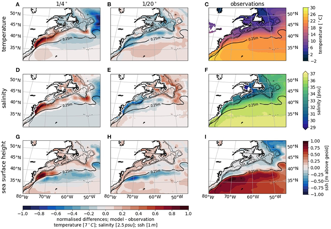
Figure 2. Surface Validation; differences between SST (A,B), SSS (D,E), and SSH (G,H) of ORCA025 (A,D,G) and VIKING20X (B,E,H) to the Observations and absolute mean Observations [OISST (C), SMOS (F), and CMEMS (I)] for the overlapping data periods from 1982 to 2019, 2010 to 2019, and 1993 to 2019, respectively; dashed lines indicate isobaths at 100, 500, and 2,000 m depth, each panel shows the CMEMS 0.25m SSH contour line for reference.
Some caveats in VIKING20X to mention are a weaker and slightly more southerly located SSH gradient across the Gulf Stream when compared to observations (Figure 2H), likely associated with a slightly smaller volume transport. The recirculation gyre in the Slope Sea off the MAB and south of Georges Bank seems to be less pronounced in the modeled SSH field. Furthermore, there is a negative surface salinity bias in VIKING20X compared to observations (Figure 2E); this is particularly pronounced along the coast, indicating that these differences may arise from differences in river runoff. Temperatures in VIKING20X depict a cold bias in the Slope Sea and on the shelf (Figure 2B). While these caveats exist, they should not have a great impact on our analysis in terms of variability. Furthermore, the improved location, in particular the separation point, of the Gulf Stream in VIKING20X compared to ORCA025 is they key for our analysis, as it greatly impacts the hydrographic representation of our focus region, the southern shelf as we will show next.
The unique long-term dataset along the Oleander line allows a cross-section validation (Figure 3). In ORCA025, warm Gulf Stream waters dominate the shelf and slope region, due to the too northerly separation point; also reflected in the broad northeastward flow over the shelfbreak and slope. Furthermore, no cold pool is found on the shelf in ORCA025 (Figure 3A). The cold water pool, characterized by temperatures below 10°C, consists of remnants of winter water being mixed downward due to surface cooling (Forsyth et al., 2015) and is an important hydrographic feature on the shelf. The mean observational Gulf Stream path intersects the Oleander line at its offshore edge (see Figure 1, 0.25 m contour line). It is visible in the cross-shelf sections of VIKING20X and the observations (Figures 3E,F). Further inshore, the slope current and surface intensified shelfbreak jet are found. Both are reproduced in VIKING20X, although slightly too strong and merged rather than separated. The former could be due to the fresh shelf bias, which likely creates a stronger cross-shelf density gradient. The sectional temperature structure including the presence of the cold pool are again much improved in VIKING20X over ORCA025.
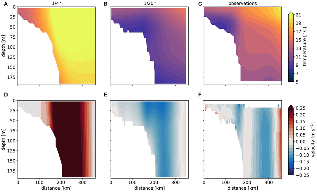
Figure 3. Subsurface validation; mean temperatures (A–C) and along shelf velocities (D–F) for ORCA025 (A,D), VIKING20X (B,E), and Observations from the Oleander Line (C,F) for the overlapping data periods from 1982–2016 to 1994–2018, respectively; velocities are positive in the north-east-direction, distance starts at Ambrose Lighthouse in New York Bay.
For further validation with respect to MHWs, surface events were detected in the temperature field of the shelf region (see ecoboxes 1–3 in Figure 1) and the total number of MHW days and the average mean intensity per year are compared between the two simulations and OISST for the overlapping time period (Figures 4A,B). As expected the higher resolution model produces much more realistic results in particular in the last decade, where the record years of 2012 (Chen et al., 2014a, 2016) and 2015/2016 (Pershing et al., 2018; Perez et al., 2021) are captured. Higher differences between all three datasets appear during the early years. ORCA025 experiences more MHWs and the intensities for both models exceed OISST. The time series of SST anomalies (Figure 4C) shows a generally good correlation of 0.8 between VIKING20X and OISST, while it is significantly lower for ORCA025 at 0.47, both significant at the 99% level. Thus, discrepancies in the number of MHW days between OISST and VIKING20X can partly be explained by the nature of defining a threshold, where the modeled SST might just pass the threshold and the observed SST is slightly below the threshold even though both show a positive SST anomaly. The differences in the SST timeseries, despite the models being forced by observations at the surface demonstrates the importance of ocean dynamics in modulating surface temperatures in this region.
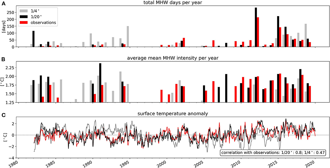
Figure 4. MHW metrics in simulations and observations; total MHW days per year (A), average mean intensity per year (B) and SST anomalies (30 day rolling window) based on the whole period for ORCA025, VIKING20X and OISST in gray, black and red, respectively for the overlapping data period from 1982-2019 (timeperiod also used as baseline for MHW detection); correlation values of the simulations to the observations are shown in (C). All metrics are based on spatially averaged temperatures over the three ecoboxes.
Overall, VIKING20X has proven to successfully reproduce key oceanographic features in the region, highlighting the importance of spatial resolution in order to resolve mesoscale ocean dynamics. Despite small differences in detected MHWs, the overall temperature structure and variability agrees well with observations, making the model suitable for our analyses.
3.2. Mean Shelf Hydrography and Trends
Considering the VIKING20X model's skillful performance in our study region, we now focus solely on this model to investigate MHWs across the entire water column on the continental shelf (<200 m). First, spatial mean seasonal profiles of modeled temperature, salinity and density over the shelf region and associated standard deviations (Figures 5A–C) are briefly analyzed to provide information on the hydrographic setting of the shelf. Note that due to the bathymetry of the shelf, upper layers (<75 m) include more data points and are more representative of shallower shoreward waters while deeper layers represent water at the shelfbreak. Although temperature generally decreases with depth, it reveals a distinct multi-layer structure with maximum temperatures at the surface, a local minimum at the bottom of the thermocline between 50 and 70 m and a subsurface maximum around 125 m depth. Salinity increases by 3.5 psu from the surface to 200 m depth with a thick halocline between approximately 50–125 m. Standard deviations for both temperature and salinity are highest at the surface and decrease with depth. Temperature and salinity profiles reflect a stable density structure. While the vertical structure is very similar between the individual ecoboxes (not shown), a distinct warming and salinification from Georges Bank to the southern MAB is in agreement with the large scale conditions and is not relevant as our analysis focuses on anomalies. The mean profiles highlight the subsurface influence of warm and saline slope/Gulf Stream water over the shelfbreak.
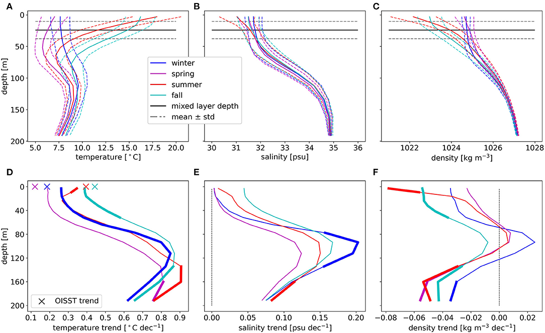
Figure 5. Shelf hydrography; seasonal and horizontal averages and standard deviations for temperature (A), salinity (B), and density (C) and mixed layer depth (A–C) plus spatial mean seasonal temperature (D), salinity (E), and density (F) trends over the shelf region (ecoboxes, see Figure 1) for the time period from 1982 to 2019; crosses in (D) mark the observed surface temperature trends, thick lines indicate significance on the 95% level.
There are pronounced seasonal differences in the shelf profiles of all three properties. Temperature (Figure 5A) is most stratified in summer and least in winter. Weak stratification throughout winter leads to the overall coldest temperatures during spring. The remnants of the cold temperatures that remain at depth while the surface warms and becomes more stratified in the following summer, are known as cold pool, which plays an important role in the seasonal variation of physical properties on the shelf (Sha et al., 2015; Chen et al., 2018) as well as, for example, species distributions (e.g., Narváez et al., 2015). Destratification of the water column occurs during fall due to surface cooling and the onset of the storm season, supplying mechanical energy for mixing. Salinity (Figure 5B) shows a freshening of around 1 psu at the surface in summer, likely associated with increased river run-off (Richaud et al., 2016). The seasonal stratification (Figure 5C) is dominated by temperature changes with a well mixed shallower shelf in winter/spring and a buoyant upper layer in summer. The modeled mean MLD is found around 25 m and its variability is mostly dominated by the seasonal cycle in temperature and salinity. It should be noted that both variables have competing and often compensating effects on density (particularly at depth) in this water mass space, which becomes very important for dynamical interpretations.
Temperature, salinity and density trends over the period from 1982 to 2019 vary over depth (Figures 5D–F). Temperature shows a linear warming of around 0.3°C per decade at the surface, which increases with depth to a trend of up to 0.9°C per decade below 120 m. These trends also change per season, especially at the surface where they are largest in fall. The significance of these trends varies depending on depth and season; winter temperature trends are significant throughout the water column, while the larger fall trend is significant in the upper layer, likely representing the shallower shelf. The seasonality of the simulated trends at the surface agrees with the satellite observations, however, there are biases of around +0.05°C in summer and fall and around –0.1°C in winter and spring. Salinity shows a similar depth structure with a salinification of around 0.03 psu per decade at the surface and up to 0.2 psu per decade at depth. These trends at depth and especially salinity are consistent with recent studies showing a northward shift of the Gulf Stream and increase of WCR interacting with the shelf (Saba et al., 2016; Gawarkiewicz et al., 2018; Gangopadhyay et al., 2019). A significant negative trend in surface density during summer indicates a temperature-driven increase in stratification. Density trends at depth are mostly insignificant, largely due to the compensation of warmer but more saline conditions at depth. What role multidecadal variability is playing in these observed trends, based on relatively short instrumental records, is an active ongoing area of research and will further be discussed throughout the manuscript.
3.3. Temporal Variability and Depth Structure of MHWs
Horizontal mean temperature and salinity anomalies across the shelf region are used to investigate MHWs, their temporal variability throughout the water column and associated salinity deviations (Figure 6). Varying depth structures are found with some MHWs being surface trapped, some occurring entirely subsurface and others extending over the full depth of the shelf. It should be noted that MHW thresholds are varying for each depth, as climatologies are derived for each z-level separately. Anomalies at depth, both positive and negative, are significantly larger than at the surface with up to ±7°C and 2 psu for temperature and salinity respectively and are centered around 100m depth. These temperature anomalies are in agreement with values observed during an advective MHW in the MAB in 2017 (Gawarkiewicz et al., 2019).
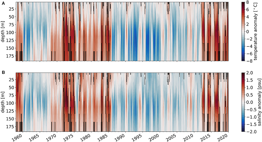
Figure 6. MHW Detection with depth; spatial mean temperature (A) and salinity anomalies (B) over depth and time for the shelf region (ecoboxes, see Figure 1); black contour lines indicate MHW state.
Salinity shows generally the same structure as temperature, in particular at depth. This covariance is consistent with the subsurface intrusions of slope water, while surface events show lower coherence with salinity (will be demonstrated more clearly in sections 3.4 and 3.5). This indicates different drivers of MHWs at different depth levels. For example air-sea interaction is more likely to impact the surface layers, as was shown for the record MHW on the shelf in 2012 (Chen et al., 2016). In contrast, oceanic processes, such as the WCR interaction with the shelf, can drive anomalies at depth (e.g., Gawarkiewicz et al., 2019). While these mechanisms have been proposed as MHW drivers based on single events, our model analysis can provide further insight as to the interannual variability of these processes and their connection to large-scale modes of variability.
Both temperature and salinity show coherent multidecadal variability of warm and saline vs. cold and fresh periods. MHW occurrence seems to follow this variability, in particular below the surface layer, meaning that long and intense MHWs mostly appear in the warm periods. Marine cold-spells (MCS) occur more frequently in the cold periods though they exhibit similar depth structures (Supplementary Figure S1). This suggests that decadal to multidecadal variability may play an important role in modulating the region's background hydrography through, for example, the diversion of fresh and cold Labrador Sea water (Holliday et al., 2020) or a shifting Gulf Stream (Neto et al., 2021) and can potentially act on top of a long term warming trend.
3.4. Statistical MHW Analysis
As a more quantitative approach we examine statistics of typical MHW metrics (duration, mean and maximum intensity) and their vertical distributions (Figure 7). This analysis provides relevant new information as to the drivers at depth, as well as for the assessment of ecosystem and fisheries impacts. The largest number of MHWs is found at the surface, however these events are also on average shorter than events at depth (Figures 7A,G) and have intensities (mean and maximum) around 2°C. The longest event in the surface layer lasts around 200 days. The number of events decreases within the upper 30 m, remains roughly constant up to 150 m depth, but increases again below. While the majority of subsurface events lasts less than 100 days, there are multiple events with a duration between 200 to 400 days. The distribution of MCSs is very similar with the highest intensities of down to –7°C at around 150 m depth (Supplementary Figure S2). Most events again occur at the surface, but only show durations of more than 100 days beneath. One difference worth mentioning is that the number of MCS events does not increase again below 150 m.
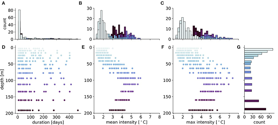
Figure 7. MHW metrics with depth; distribution of MHW duration (D), mean intensity (E) and maximum intensity (F) with depth for each detected MHW during 1960–2019, averaged across the shelf (ecoboxes, see Figure 1); (A–C) show the distribution for each metric in the color for each depth as in (D–F); (G) shows the total count of MHWs for each depth.
These distributions do not account for vertical coherence of MHWs. However, the long events seem to span across the majority of the water column and are limited to the prolonged warm phases (Figure 6). This indicates a modulation of the region's background state on longer time scales which becomes more or less favorable for MHW generation. The surface layer is generally more influenced by air-sea forcing varying on a shorter synoptic timescale, explaining the shorter duration but higher frequency of events. A synoptic event passing through may decrease the SST for more than two consecutive days (interrupting the MHW), while subsurface anomalies remain above the threshold. Hence multiple surface MHWs may occur during a prolonged subsurface MHW. Alternatively, in the presence of strong stratification during summer, short-term increases in surface heat flux can induce a MHW, which is then terminated by a change in air-sea forcing.
For ecological purposes surface events may not be as relevant as temperature anomalies at depth. Mean and maximum intensities mostly vary around 1–3°C in the upper layers (Figures 7E,F), while a maximum at 100 m depth is associated with anomalies ranging between 3.5 and 7.0 °C. Below 100m depth, intensities decrease again, but remain higher than the surface values. Thus, the thermal stress associated with a MHW at depth can be substantially higher. The number of detected events increases in the two lower levels, which can be explained by the mechanism that drives these subsurface anomalies (as shown in the results and discussion). Ultimately, it will be important to assess the relevance of short (order of days) vs. long (order of months) MHWs, also in relation to their frequency. It may not just be the long MHWs that are most devastating but also multiple consecutive short events, where the temperature drops just below the threshold in between can still exert considerable thermal stress on the ecosystem over an extended period of time. However, this is rather speculative and warrants further investigation in future studies.
Investigating the co-variability of temperature and salinity can give further insight into MHW drivers and water masses involved (Figure 8A). Both, temperature and salinity have competing effects on density and thus on the shelf stratification as well as lateral density gradients, which are dynamically important. Salinity extremes are detected using the 90th (10th) percentile to be consistent with the MHW (MCS) definition. More than 80% of MHWs below roughly 75 m depth co-occurred with a positive salinity extreme, again supporting the influence of warm and salty slope/Gulf stream waters at depth. The percentage of co-occurrence decreases gradually toward the surface to about 40%, where additional processes become relevant. The overall distribution of temperature and salinity anomalies (Figure 8B) shows a connection between warm and salty vs. cold and fresh anomalies, especially in the extreme values associated. At the surface, MHWs also occur in conjunction with fresh anomalies, which might be attributed to a shoaling of the mixed layer due to anomalous surface freshwater input. The symmetry at depth suggests once more the strong influence of off-shelf waters at mid-depth; shelf processes alone are unable to produce such strong anomalies and, as noted already, the conditions at depth are representative of the outer shelf. The cold and fresh extremes, which co-occur at depth up to 80% of the time as well, may be generated by a period of anomalously reduced WCR interaction or internal variations of the shelf advection and associated water mass properties. However, the quantification of WCR impact on the shelf and connectivity to large-scale climate variability is ongoing research (Gangopadhyay et al., 2019; Silver et al., 2021).
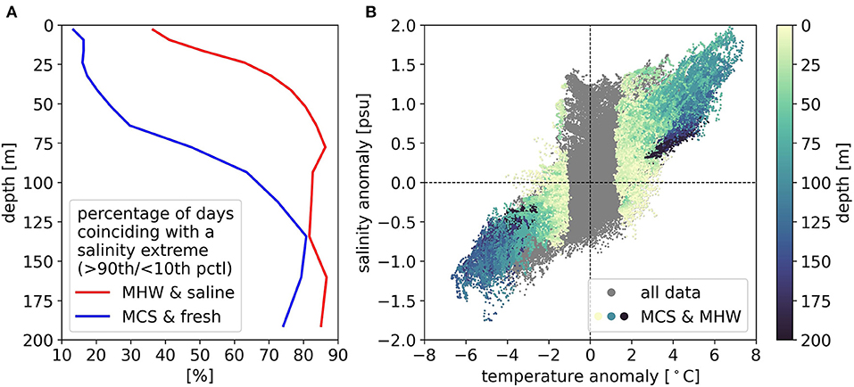
Figure 8. Co-variability of heat and salinity extremes and general anomalies; percentage of MHW (MCS) days coinciding with a saline (fresh) extreme for each depth level (A) [salinity extreme detection with the same mechanism as for MHWs (MCSs)]; temperature-salinity-plot for anomalies (B) for all the data; MHW (positive temperature anomalies) and MCS (negative temperature anomalies) points are colored by their depth; note that MHW and MCS points can overlay gray points with large anomalies, though they are not detected as extremes given the season and/or depth.
To assess seasonal differences in MHW occurrence, the average number of MHW days throughout the simulation are derived for each season (Figure 9). Besides providing more information on forcing mechanisms, seasonality can be of particular importance for the ecosystem. For example, at what life stages organisms experience temperature anomalies or where migrating species reside/spawn during a specific time of year can determine an MHW's ecological impact. Note that the seasonally varying climatology is used for MHW detection. Therefore, the warmer summer temperatures themselves do not favor MHW occurrence. The largest variability is seen in the upper layers (<75 m), which is likely driven by seasonal changes in stratification and halocline depth (cf. Figure 5C). Most surface layer (<30 m) MHW days occur during summer. The local maximum is located right beneath the shallow mixed layer, which could be due to wind events mixing the warm surface waters deeper into the thermocline. MHW days during the shoulder seasons in March-May and September-October are likely connected to changes in timing of the stratification build-up after winter or the destratification process in fall. Furthermore, the maximum number of MHW days is found just below the surface, which, as mentioned earlier, is likely due to the increased SST variability driven by surface fluxes. The deeper layers seem to experience less seasonal variations in terms of MHW days. However, intensities at depth are largest in the fall (SON) agreeing with previous findings of increased WCR births in summer (Zhai et al., 2008; Gangopadhyay et al., 2019). Once formed, the WCRs then have to travel for some time before reaching the investigated shelf regions to intrude their warm waters on the shelf at depth, forcing a MHW in SON. The seasonal distribution of the mean intensity for salinity extremes has its maximum at 100 m in SON as well, underlining this theory. Furthermore the largest number of mid-depth salinity intrusions is observed during August and September (Lentz, 2003). MCS events show the opposite structure on the surface with most days in winter and spring, while the signal at depth is similar (Supplementary Figure S3). Highest intensities can be found at around 100 m depth during summer.
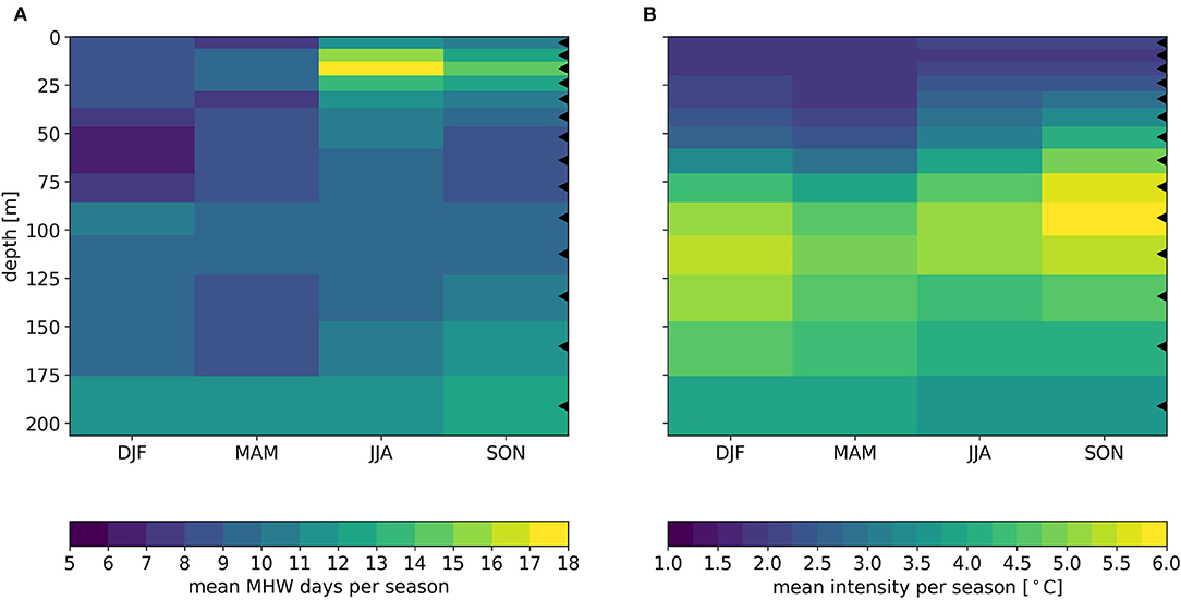
Figure 9. Seasonal distribution of total MHW days (A) and mean intensity per season (B) with depth (averaged over ecoboxes, see Figure 1); markers on the right indicate depth levels of the model. Acronyms for seasons are: December, January, and February (DJF), March, April, and May (MAM), June, July, and August (JJA), and September, October, and November (SON).
3.5. Case Studies: Different MHW Types
Our analysis suggests that different drivers may be responsible for MHWs at different depth levels. As explained above, we distinguish the upper layer extending from the surface to about 30 m depth (representing the average MLD) from the lower layer from below 75 m downward, associated with the geometry of the shelf. In order to gain a more mechanistic understanding of the drivers of the different types of MHWs, i.e., the surface and subsurface, we now present two case studies and will also investigate the spatial structure over the shelf by introducing a new metric.
In 2002, multiple MHW events confined to the upper layers (<50 m) were detected between February and October. In contrast, January to October 2014 was characterized by a prolonged and almost entirely subsurface MHW. A new metric is introduced to visualize the 3D spatial extent of a MHW: the percentage of the water column in MHW state throughout the analyzed period (Figure 10). Note, this does not provide information as to which parts of the water column are in MHW state. Furthermore, one has to keep in mind, that the shelf deepens offshore, hence a surface MHW may occupy the whole water column in the shallower part of the shelf but will be associated with a smaller fraction over the deeper part. Nevertheless, this new metric provides a novel way to analyze the 3D structure of MHWs and together with Hovmoeller plots of the box-averaged temperature, salinity and density anomalies (Figures 11, 12), this is informative for the overall spatio-temporal structure and evolution of a MHW.
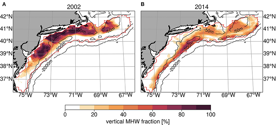
Figure 10. Vertical MHW fraction of events in 2002 (A) and 2014 (B); temporal and depth-weighted mean of MHW occurrence; dashed lines indicate isobaths for 50, 200, and 2,000 m depth. Note that only data within the red outline (ecoboxes) is used here.
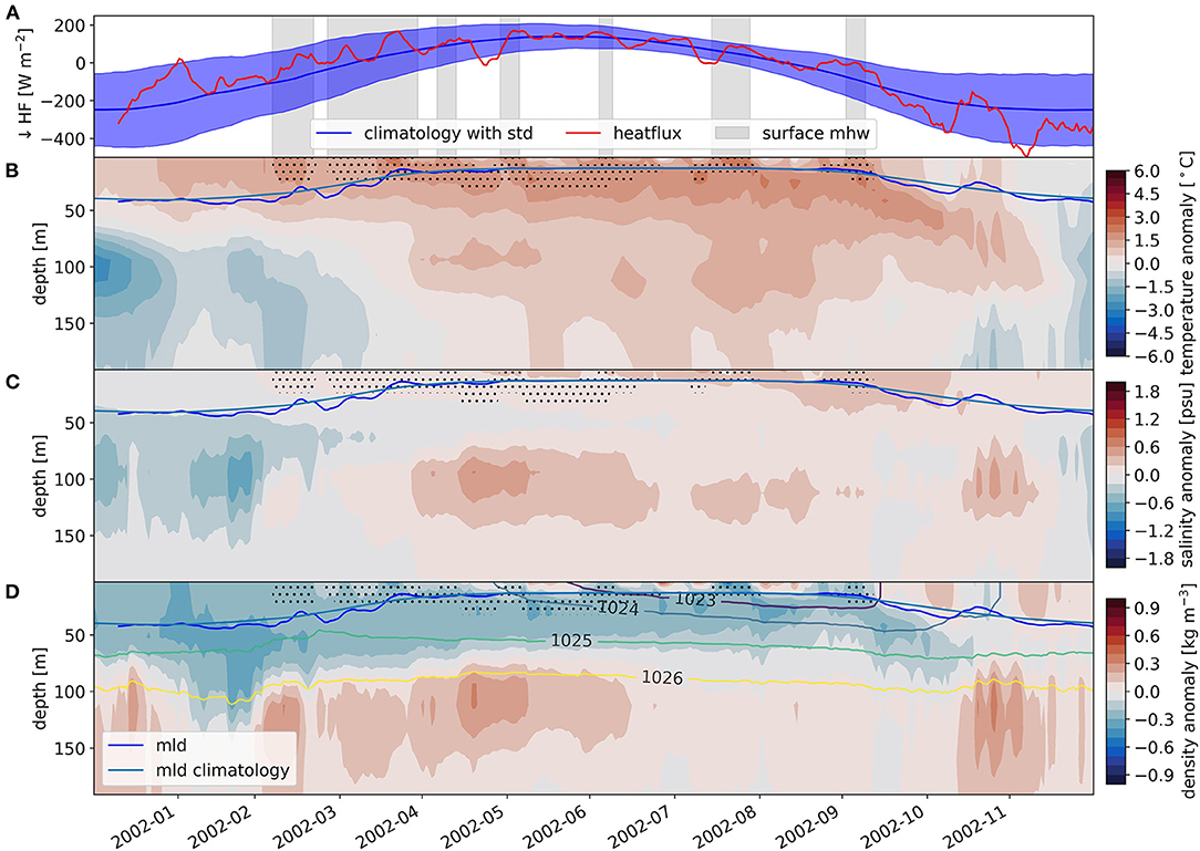
Figure 11. 2002 MHW characteristics; time series of net downward surface heat flux (A) and hovmoeller plots for temperature (B), salinity (C), and density (D) anomalies with depth over time for 2002; (A) contains the heat flux from the current year and the heat flux climatological values; light and dark blue line (B–D) show mixed layer depth from climatology and in 2002; labeled contour lines in (D) show absolute densities, stippling indicates MHW state; 10 day rolling window for heatflux and mixed layer depth time series. Values displayed represent an average over the shelf (ecoboxes, see Figure 1).
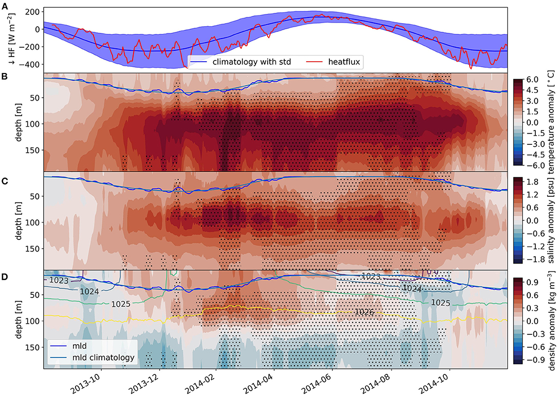
Figure 12. 2014 MHW characteristics; time series of net downward surface heat flux (A) and hovmoeller plots for temperature (B), salinity (C), and density (D) anomalies with depth over time for 2014; (A) contains the heat flux from the current year and the heat flux climatological values; light and dark blue line (B–D) show mixed layer depth from climatology and in 2014; labeled contour lines in (D) show absolute densities, stippling indicates MHW state; 10 day rolling window for heatflux and mixed layer depth time series. Values displayed represent an average over the shelf (ecoboxes, see Figure 1).
Both events have distinctly different spatial structures. The MHW in 2002 mostly affects the central MAB as well as the eastern Georges Bank (Figure 10A). Furthermore, it is focused on the shallower shelf (inshore of the 70 m isobath) without a signature along the shelfbreak. In some shallow regions, the whole water column experiences MHW conditions. The temporal evolution of the distribution (Supplementary Figure S4 and Video S1) shows that the MHW started on the coast, then extends offshore, but never reached the shelfbreak. The Hovmoeller plot and downward heat flux timeseries suggest that the onset of the MHW was driven by a prolonged period of anomalously positive heat flux into the ocean (reduced heat loss), with a stronger peak between December 2001 and January 2002. As reference, the heat flux anomaly is almost double compared to the onset of the 2012 event. Positive anomalies last until April 2002 intensifying surface temperatures anomalies (up to 2°C) and likely maintaining the MHW. Salinity anomalies are slightly positive around 0.5 psu and the upper 70 m of the water column generally depicts a negative density anomaly, while the lower layer shows a positive density anomaly, indicative of an overall increased stratification. The MLD does not show a shoaling signal, though this can be attributed to the spatial averaging. Monthly maps of MLD anomalies (not shown) reflect a shoaling over the shallower shelf region where the MHW is formed. From roughly March to June the surface layer drops in and out of MHW state multiple times while the subsurface layer remains in MHW state. As mentioned earlier, the shallow mixed layer in summer is likely more modulated by air sea heat fluxes, which fluctuate around the climatological mean during that time. The second half of the summer (June onward) is still characterized by positive temperature anomalies, however MHW state is only entered sporadically. In Mid-November, the anomalies start decaying at the surface and slightly deepen in conjunction with the onset of negative heat fluxes, which also drives a gradual destratification. While being beyond the scope of this study, the process and timing of seasonal destratification and associated drivers, such as an increase in storm frequency, likely play an important role for the decay of MHWs, in particular for those confined to the surface layer.
The year 2014 experienced a MHW with a very different spacial structure, compared to 2002. The entire shelfbreak and outer shelf are impacted while the shallower, shoreward region is mostly unaffected, in particular in the southern MAB (Figure 10B). Furthermore, not the entire water column is in MHW state, which also stands out in the Hovmoeller plot. Temperature anomalies are highest around 100 m depth with magnitudes as high as 6°C, and anomalies around 5°C persisting throughout the entire time between Dec 2013 and Oct 2014. Positive anomalies are found in the whole water column throughout the period, however the upper layer is not in MHW state until June when the MHW extends to the base of the shallow mixed layer. Typically the summer surface warming begins and climatological heat fluxes are at their maximum. Surface heat fluxes in the preceding winter season mostly stay below or close to the climatological mean, suggesting that this MHW is of oceanic origin. Salinity has a very similar structure with anomalies reaching up to 2 psu at depth, again indicating the influence of warm and saline Slope/Gulf Stream waters. The monthly evolution of the velocity field and vertical MHW fraction for the upper 500 m show a WCR forming in Oct 2013. The WCR impinges on the shelfbreak in Jan/Feb 2014 creating a warm anomaly that is advected southwestward along the shelfbreak (Supplementary Figures S5 and Video S2). From July onward, new positive anomalies appear upstream at Georges Bank which again propagate southward but also intrude further onto the shelf, which could drive the observed expansion into shallower depth of the MHW during that time. In October, the MHW state in the upper layer ends, associated with anomalous surface heat loss, likely driven by the seasonal changes; that is, a cooling atmosphere and increased surface wind stress during fall. At depth (~ 100 m) the MHW ends in October. Indeed looking at the spatial distribution (Supplementary Figure S5) the WCR reached the southern MAB at that time and has diminished visibly.
The two presented MHW types are summarized in a schematic (Figure 13), highlighting the relative roles of air-sea heat fluxes and the WCR interaction with the shelf, driving surface and subsurface MHWs, respectively. While the case-studies highlight “pure” forms of these different MHW types, there are likely many events where both processes contribute, which should be a subject of future research.
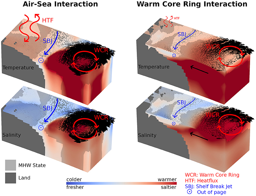
Figure 13. Schematic of the two dominating MHW structures and related drivers in the region; shown are 3D fields of temperature and salinity anomalies with shaded MHW state, surface arrows indicate velocities.
4. Discussion and Conclusions
The Northeast U.S. continental shelf is among the fastest warming regions in the global ocean (Saba et al., 2016). Consequently, it experienced multiple MHWs over the last decade (e.g., Chen et al., 2014a; Gawarkiewicz et al., 2019), affecting the rich regional ecosystem and ultimately commercial fisheries (Pershing et al., 2015). Previous studies identified ocean warming as the major cause of distribution changes of marine species (e.g., Pinsky et al., 2013; Hare et al., 2016), however it has also been suggested that relying on temperature only can significantly mask species' climate vulnerability (McHenry et al., 2019). While distribution shifts are likely driven by a mean change in climate velocity, defined by the mean direction and speed of changes in the physical habitat (Pinsky et al., 2013), extreme events like MHWs may have irreversible consequences on individual species and, as shown in 2012, severe economic impacts. Furthermore, MHWs can serve as a “real life” sensitivity experiment in order to investigate local ecosystem responses to a potentially permanent stage in the future.
Limited subsurface observations hinder a full 3D assessment of MHWs and their evolution temporally and spatially over the slope and shelf region. Yet, that is crucial in order to address their potential consequences, in particular for pelagic and benthic fish species and organisms. Here, climate and ocean models can serve as a valuable tool, however the complexity of the region's circulation and bathymetry requires high spatial and vertical resolution. As a result, typical climate models are too coarse and show large biases in the Northwest Atlantic, largely associated with a Gulf Stream separation too far north (Wang et al., 2014; Saba et al., 2016). Our model comparison confirms this and highlights the need of high-resolution simulations. The presented state-of-the-art high resolution ocean model at 1/20° spatial and daily temporal resolution has proven successful in resolving the region's circulation and hydrography accurately.
This study is by no means aiming to provide detailed insights into shelfbreak dynamics, which likely requires spatial resolutions on the order of 1 km and more dedicated regional modeling approaches (e.g., Chen et al., 2022). However, our validation shows that VIKING20X reproduces the key regional oceanographic features and this study can therefore serve as a proof-of-concept and provides a baseline for future MHW studies in the region, highlighting how important regional and full-depth MHW studies are in particular in such complex regions. It is of great importance to understand the specifics of the regional circulation and it's connection to large-scale ocean circulation, climate variability and trends.
We present a first comprehensive picture of traditional MHW metrics across depths in the MAB and Georges Bank region and provide a novel metric to combine the spatial and vertical extent of a MHW. We find that intensities are considerably greater at depth, typically ranging between 4 and 6°C and maximum intensities of up to 7°C, while surface intensities range between 1 and 3°C. The majority of events lasts shorter than 30 days. Particularly at the surface, events tend to be shorter but also more frequent, which is likely because of the direct influence of air-sea forcing which varies on a shorter synoptic timescale. Across all depths, we find events lasting longer than 100 days with maximum duration of 400 days. To be able to fully assess impacts on the ecosystem and the role of, for example, short and intense versus long and less intense events (but potentially high cumulative heat flux), one has to understand species' sensitivities to thermal stress. While it has been shown that the mean warming on the shelf has caused a northward or offshore shift of many marine species (e.g., Nye et al., 2009; Pinsky et al., 2013), the impacts of temperature extreme events may be more complex to assess. Most species have an upper (and lower) thermal tolerance threshold for example the American Lobster (Homarus americanus) prefers temperatures below 18°C and shows signs of biological stress above 20°C (Dove et al., 2005). Hence the absolute temperatures associated with MHWs can be more important than anomalies; furthermore, in regions with a large seasonal cycle in temperature these thresholds will be exceeded more easily in some seasons compared to others.
The seasonal analysis presented here (Figure 9) shows that the upper layer (<30 m) experiences more MHW days in summer and fall, with the fewest MHW days in winter. This is likely associated with the mean temperature trend being largest in fall, while trends in other seasons are not significant (see Figure 5D and Kleisner et al., 2017; Friedland et al., 2020). Considering the season in which MHWs occur can be important because of impacts on phenology, that is different life stages of species. For example, reproduction of most temperate species begins in spring and summer, yet is strongly temperature driven (Thorson, 1950; Olive, 1995). Therefore, anomalous warming earlier in the year can lead to an early onset of spawning, as observed recently (Philippart et al., 2003; Asch, 2015), which in turn can cause “wrong-way” migrations because larvae are exposed to different ocean transports on the shelf (Fuchs et al., 2020). At depth (>80 m) we find less seasonal variability in MHW days, although intensities are largest in fall and occur slightly shallower. In this study, we establish that these anomalies at depth are somewhat decoupled from surface processes and are instead mainly driven by shelf break exchange, i.e., intrusions of warm and saline Gulf Stream originating slope water. This apparent 2-layer system may be an artifact due to the spatial averaging of conditions over the whole shelf up to the shelf break at the 200 m isobath. A large part of the shelf, in particular in the southern MAB is shallower than 70 m.
Two presented case-studies elaborate further on different types of MHWs found on the Northeast U.S. continental shelf which are associated with the geometry of the shelf and different forcing mechanisms. Even though SST is generally a good proxy for thermal conditions in shallow waters, seasonal stratification and lateral differences in current flow can drive a decoupling of surface and bottom temperatures, in particular in deeper parts of the shelf. Thus, it is important to distinguish different types of MHWs and understand drivers across depth to fully assess impacts on pelagic and benthic organisms. A series of surface intensified MHWs in 2002 (Figure 11) was associated with anomalous surface heat flux into the ocean, the process that is suggested to be responsible for the onset of about 50% of observed surface MHWs (Schlegel et al., 2021) in this region. Our spatial analysis (Figure 10A) shows that the 2002 MHW occupied a large part of the water column on the inner shelf, shoreward of the 70 m isobath while the shelfbreak was not affected. In the deeper troughs the vertical MHW fraction is reduced, indicating that the deeper levels here are generally not in MHW state. In contrast in 2013–2014 a pure subsurface MHW is associated with temperature and salinity maxima at about 100 m depth and our results suggest that these are driven by intrusions of warm and saline slope water along the shelfbreak which are then advected southward via the shelfbreak jet; a WCR is found to impinge on the continental shelf during that time. Furthermore, we find that below approximately 75 m depth over 80% of MHW days coincide with positive salinity extremes. It has been shown previously that these interactions frequently impact the shelf's hydrography and can cause large cross-shelf heat and salt-fluxes and mid-depth intrusions (Gawarkiewicz et al., 2001; Lentz, 2003; Chen et al., 2014b; Zhang and Gawarkiewicz, 2015). Furthermore, these results are consistent with an observed advective MHW on the shelf in 2017, also induced by a WCR (Gawarkiewicz et al., 2019; Chen et al., 2022). It should be noted that the slope region was generally very warm during 2014 (and preceding years), in the model (not shown) as well as in observations (Chen et al., 2020; Seidov et al., 2021). This may be related to a number of interconnected processes: an increased number of WCRs (Gangopadhyay et al., 2019), a westward shift of the destabilization point of the Gulf Stream (Andres, 2016) and a northward shift of the Gulf Stream (Neto et al., 2021) associated with a slowdown of the meridional overturning circulation (Caesar et al., 2018). Hence, even if there is no direct contact of a WCR with the shelf break, a subsurface MHW could also be driven by enhanced cross-shelf transport of the anomalously warm slope water. However, cross-shelf intrusions are governed by complex shelf-break dynamics and generally require special conditions, such as the set-up of a along-shelf pressure gradient that can facilitate cross-shelf flow (Chen et al., 2022) as the mean flow is largely geostrophic along isobaths (e.g., Lentz, 2008).
Based on the time evolution of spatially averaged temperature and salinity anomalies in Figure 6, our results suggest that subsurface MHWs only occur during prolonged warm phases of the shelf. These are likely associated with multidecadal variability of the Northwest Atlantic. Based in SSH observations, it has been shown that a recent northward shift of the Gulf Stream in 2008 lead to an abrupt warming of the Northwest Atlantic Shelf due to a reduction of cold and fresh water supply via the Labrador Current near the Tail of Grand Banks (Neto et al., 2021). The temperature shift in the MAB occurred toward the end of 2011 (Figure 3 therein; Neto et al., 2021), which is in good agreement with the modeled variability and also marks the beginning of the onset of frequent and long subsurface MHWs, in conjunction with strong positive salinity anomalies, in the recent decade. Simultaneously, Holliday et al. (2020) describe a fresh anomaly propagating into the subpolar eastern Atlantic from the Tail of Grand Banks between 2012 and 2016. They propose that anomalously strong wind stress curl over the subpolar North Atlantic caused a re-routing of Arctic-originating freshwater. Furthermore, an EOF (Empirical Orthogonal Function) analysis of the upper 200 m annual mean salinity from 1945 to 2015 (Figure 6 therein; Holliday et al., 2020) reveals a characteristic dipole structure between the subpolar North Atlantic and the North Atlantic continental shelf and slope region, whose principal component timeseries compares well to our modeled variability. This strengthens our confidence in the model but more importantly underlines that interannual to multidecadal variability in the MAB is connected to basin-scale circulation changes. As mentioned earlier, the occurrence of subsurface MHWs (MCSs) seems to be linked to these warm (cold) phases. Hence, if a WCR interacts with the shelfbreak in a cold phase, it may drive an anomaly but not an extreme event. However, in a warm phase, it will act on top of a warm background state and can thus generate an extreme event. Furthermore, this long-term variability can impact the detection of MHWs depending on the chosen baseline. While we did not elaborate on this in our study, it is evident that if the baseline was chosen from 1983 to 2012 (used in many MHW studies), the MHWs detected in the recent warming phase would have been even more extreme. Generally the baseline should be chosen with respect to its context in particular for the assessment of ecosystem impacts, where one has to consider the adaptability of species to temperature changes.
Although the modeled variability agrees well with existing studies, it should be noted that the presented simulations started from a resting ocean (i.e., no spin-up). Therefore, the first 20–30 years should be treated with caution, in particular for absolute values or trends, while the general variability seems realistic as discussed above. The shallow shelf region can be expected to adjust within a few years which is why we chose to analyze the full time period, which allowed us to address the role of long-term variability but also provided us with more data points for the MHW statistics. All statistics were also performed with data only from 1980 onward, however we did not find any notable changes in the vertical distributions, which gives additional confidence in our results. Various studies have shown an accelerated warming on the Northeast U.S. continental shelf in the recent decade (e.g., Saba et al., 2016; Chen et al., 2020), which also was identified as a driver for the strong observed coastal warming in the Northeast U.S. (Karmalkar and Horton, 2021). The modeled anomalies in the two warm phases from roughly 1972 to 1985 and from 2012 onward are of the same magnitude, which may indicate a slight warm bias in the model during this time, likely connected to the ongoing spin-up of the large-scale circulation. Nevertheless, we are confident that the new insights provided in this study as to the different vertical types of MHWs and their drivers remain valid and that the overall results serve not only as an important baseline for studying extreme events, but also temperature variability in general in this region. Next steps could be a more quantitative approach on the role of WCRs vs. variability in shelf advection in driving MHWs either directly or via preconditioning. It will be important to decouple trend signals from long-term variability. Recent studies highlight that climate models currently do a poor job in western boundary regions (e.g., Hayashida et al., 2020), which can lead to substantial biases in climate projections for this region; thus dedicated regional studies are indispensable.
Data Availability Statement
Publicly available datasets were analyzed in this study. This data can be found here: NOAA High Resolution SST data v2.1 provided by the NOAA/OAR/ESRL PSL, Boulder, Colorado, USA, from their website at https://psl.noaa.gov/data/gridded/data.noaa.oisst.v2.highres.html. The XBT data product, gridded and monthly averaged from 1977 to 2018, is available at https://doi.org/10.5281/zenodo.3967332, the raw CMV Oleander data is available at http://oleander.bios.edu/data/. Global ocean gridded L4 sea surface heights, which is made available by E.U. Copernicus Marine Service (CMEMS) and can be downloaded under https://resources.marine.copernicus.eu/?option5com_csw&task5results?option5com_csw&view5details&product_id5SEALEVEL_GLO_PHY_L4_REP_OBSERVATIONS_008_047. The SMOS L3_DEBIAS_LOCEAN_v5 Sea Surface Salinity maps have been produced by LOCEAN/IPSL (UMR CNRS/SU/IRD/MNHN) laboratory and are available at https://www.seanoe.org/data/00417/52804/. The MHW detection algorithm was originally written by Eric C. J. Oliver (https://github.com/ecjoliver/marineHeatWaves). The adapted code used here by Paola Petrelli can be found at https://zenodo.org/record/5112733#.YdYKVVlOmF4. For reproducibility of all results, code (jupyter notebooks) and data required to produce the figures are made available through a THREDDS server at GEOMAR at https://hdl.handle.net/20.500.12085/b61b44fe-f4c8-4834-9c7f-91a5a9363b25.
Author Contributions
HG and SR led the paper equally and wrote and structured the manuscript. HG performed all the analyses under guidance of SR. All authors discussed the analyses and provided comments to the text.
Funding
This work was supported by a DAAD RISE Worldwide fellowship (to HG), a Feodor-Lynen Fellowship by the Alexander von Humboldt Foundation and the WHOI Postdoctoral Scholar program (to SR), and the James E. and Barbara V. Moltz Fellowship for Climate-Related Research (to CU). Franziska Schwarzkopf performed the integration of the OGCM simulations, which was performed on the Earth System Modeling Project (ESM) partition of the supercomputer JUWELS at the Jülich Supercomputing Centre (JSC).
Conflict of Interest
The authors declare that the research was conducted in the absence of any commercial or financial relationships that could be construed as a potential conflict of interest.
Publisher's Note
All claims expressed in this article are solely those of the authors and do not necessarily represent those of their affiliated organizations, or those of the publisher, the editors and the reviewers. Any product that may be evaluated in this article, or claim that may be made by its manufacturer, is not guaranteed or endorsed by the publisher.
Acknowledgments
The authors are thankful to Paola Petrelli for her support of the MHW detection code. Discussions with Glen Gawarkiewicz and Paula Fratantoni are greatly appreciated. The authors would also like to thank both reviewers for their time and constructive comments.
Supplementary Material
The Supplementary Material for this article can be found online at: https://www.frontiersin.org/articles/10.3389/fclim.2022.857937/full#supplementary-material
Video S1. Monthly mean modeled surface velocities and vertical MHW fraction for the upper 500 m for each month during the MHW in 2002, the black line indicates the 200m isobath.
Video S2. Monthly mean modeled surface velocities and vertical MHW fraction for the upper 500 m for each month during the MHW in 2014, the black line indicates the 200m isobath.
References
Amante, C., and Eakins, B. (2009). ETOPO1 1 Arc-Minute Global Relief Model: Procedures, Data Sources and Analysis. NOAA Technical Memorandum NESDIS NGDC-24, March 19.
Andres, M. (2016). On the recent destabilization of the Gulf Stream path downstream of Cape Hatteras. Geophys. Res. Lett. 43, 9836–9842. doi: 10.1002/2016GL069966
Andres, M., Donohue, K. A., and Toole, J. M. (2020). The Gulf Stream's path and time-averaged velocity structure and transport at 68.5°W and 70.3°W. Deep Sea Res. I Oceanogr. Res. Papers 156, 103179. doi: 10.1016/j.dsr.2019.103179
Asch, R. G. (2015). Climate change and decadal shifts in the phenology of larval fishes in the California Current ecosystem. Proc. Natl. Acad. Sci. U.S.A. 112, E4065–E4074. doi: 10.1073/pnas.1421946112
Banzon, V., Smith, T. M., Mike Chin, T., Liu, C., and Hankins, W. (2016). A long-term record of blended satellite and in situ sea-surface temperature for climate monitoring, modeling and environmental studies. Earth Syst. Sci. Data 8, 165–176. doi: 10.5194/essd-8-165-2016
Barnier, B., Madec, G., Penduff, T., Molines, J. M., Treguier, A. M., Le Sommer, J., et al. (2006). Impact of partial steps and momentum advection schemes in a global ocean circulation model at eddy-permitting resolution. Ocean Dyn. 56, 543–567. doi: 10.1007/s10236-006-0082-1
Biastoch, A., Schwarzkopf, F. U., Getzlaff, K., Rühs, S., Martin, T., Scheinert, M., et al. (2021). Regional imprints of changes in the Atlantic Meridional Overturning Circulation in the eddy-rich ocean model VIKING20X. Ocean Sci. 17, 1177–1211. doi: 10.5194/os-17-1177-2021
Boutin, J., Vergely, J.-L., and Khvorostyanov, D. (2020). SMOS SSS L3 maps generated by CATDS CEC LOCEAN. debias V7.0. doi: 10.17882/52804
Boutin, J., Vergely, J. L., Marchand, S., D'Amico, F., Hasson, A., Kolodziejczyk, N., et al. (2018). New SMOS Sea Surface Salinity with reduced systematic errors and improved variability. Remote Sens. Environ. 214, 115–134. doi: 10.1016/j.rse.2018.05.022
Breckenfelder, T., Rhein, M., Roessler, A., Böning, C. W., Biastoch, A., Behrens, E., et al. (2017). Flow paths and variability of the North Atlantic Current: a comparison of observations and a high-resolution model. J. Geophys. Res. Oceans 12, 2686–2708. doi: 10.1002/2016JC012444
Caesar, L., Rahmstorf, S., Robinson, A., Feulner, G., and Saba, V. (2018). Observed fingerprint of a weakening Atlantic Ocean overturning circulation. Nature 556, 191–196. doi: 10.1038/s41586-018-0006-5
Chen, K., Gawarkiewicz, G., and Yang, J. (2022). Mesoscale and submesoscale shelf-ocean exchanges initialize an advective marine heatwave. J. Geophys. Res. Oceans 127, e2021JC017927. doi: 10.1029/2021JC017927
Chen, K., Gawarkiewicz, G. G., Kwon, Y.-O., and Zhang, W. (2015). The role of atmospheric forcing versus ocean advection during the extreme warming of the Northeast U.S. continental shelf in 2012. J. Geophys. Res. Oceans 120, 4324–4339. doi: 10.1002/2014JC010547
Chen, K., Gawarkiewicz, G. G., Lentz, S. J., and Bane, J. M. (2014a). Diagnosing the warming of the Northeastern U.S. Coastal Ocean in 2012: a linkage between the atmospheric jet stream variability and ocean response. J. Geophys. Res. Oceans 119, 218–227. doi: 10.1002/2013JC009393
Chen, K., He, R., Powell, B. S., Gawarkiewicz, G. G., Moore, A. M., and Arango, H. G. (2014b). Data assimilative modeling investigation of Gulf Stream Warm Core Ring interaction with continental shelf and slope circulation. J. Geophys. Res. Oceans 119, 5968–5991. doi: 10.1002/2014JC009898
Chen, K., Kwon, Y., and Gawarkiewicz, G. (2016). Interannual variability of winter-spring temperature in the Middle Atlantic Bight: Relative contributions of atmospheric and oceanic processes. J. Geophys. Res. Oceans 121, 4209–4227. doi: 10.1002/2016JC011646
Chen, Z., Curchitser, E., Chant, R., and Kang, D. (2018). Seasonal Variability of the Cold Pool Over the Mid-Atlantic Bight Continental Shelf. J. Geophys. Res. Oceans 123, 8203–8226. doi: 10.1029/2018JC014148
Chen, Z., Kwon, Y. O., Chen, K., Fratantoni, P., Gawarkiewicz, G., and Joyce, T. M. (2020). Long-term SST variability on the northwest atlantic continental shelf and slope. Geophys. Res. Lett. 47, 1–11. doi: 10.1029/2019GL085455
Csanady, G. T., and Hamilton, P. (1988). Circulation of slopewater. Cont Shelf Res. 8, 565–624. doi: 10.1016/0278-4343(88)90068-4
Dove, A. D., Allam, B., Powers, J. J., and Sokolowski, M. S. (2005). A prolonged thermal stress experiment on the American lobster, Homarus americanus. J. Shellfish Res. 24, 761–765. doi: 10.2983/0730-8000(2005)24<761:APTSEO>2.0.CO;2
Ecosystem Assessment Program (2012). Ecosystem Status Report for the Northeast Shelf Large Marine Ecosystem-2011. U.S. Deptartment of Commerce, Northeast Fisheries Science Center Reference Documents 12–07.
Elzahaby, Y., and Schaeffer, A. (2019). Observational insight into the subsurface anomalies of marine heatwaves. Front. Mar. Sci. 6, 745. doi: 10.3389/fmars.2019.00745
Fichefet, T., and Maqueda, M. A. (1997). Sensitivity of a global sea ice model to the treatment of ice thermodynamics and dynamics. J. Geophys. Res. Oceans 102, 12609–12646. doi: 10.1029/97JC00480
Flagg, C. N., Dunn, M., Wang, D.-P., Rossby, H. T., and Benway, R. L. (2006). A study of the currents of the outer shelf and upper slope from a decade of shipboard ADCP observations in the Middle Atlantic Bight. J. Geophys. Res. 111, C06003. doi: 10.1029/2005JC003116
Forsyth, J., Andres, M., and Gawarkiewicz, G. (2020). Shelfbreak jet structure and variability off New Jersey using ship of opportunity data from the CMV oleander. J. Geophys. Res. Oceans 125, e2020JC016455 doi: 10.1029/2020JC016455
Forsyth, J., Andres, M., and Gawarkiewicz, G. G. (2015). Recent accelerated warming of the continental shelf off New Jersey: Observations from the CMV Oleander expendable bathythermograph line. J. Geophys. Res. C Oceans 120, 2370–2384. doi: 10.1002/2014JC010516
Fratantoni, P. S., and Pickart, R. S. (2007). The western North Atlantic shelfbreak current system in summer. J. Phys. Oceanogr. 37, 2509–2533. doi: 10.1175/JPO3123.1
Friedland, K. D., Morse, R. E., Manning, J. P., Melrose, D. C., Miles, T., Goode, A. G., et al. (2020). Trends and change points in surface and bottom thermal environments of the US Northeast Continental Shelf Ecosystem. Fish. Oceanogr. 29, 396–414. doi: 10.1111/fog.12485
Fuchs, H. L., Chant, R. J., Hunter, E. J., Curchitser, E. N., Gerbi, G. P., and Chen, E. Y. (2020). Wrong-way migrations of benthic species driven by ocean warming and larval transport. Nat. Clim. Chang 10, 1052–1056. doi: 10.1038/s41558-020-0894-x
Gangopadhyay, A., Gawarkiewicz, G., Silva, E. N. S., Monim, M., and Clark, J. (2019). An observed regime shift in the formation of warm core rings from the gulf stream. Sci. Rep. 9, 1–9. doi: 10.1038/s41598-019-48661-9
Gawarkiewicz, G., Bahr, F., Beardsley, R. C., and Brink, K. H. (2001). Interaction of a slope eddy with the shelfbreak front in the Middle Atlantic Bight. J. Phys. Oceanogr. 31, 2783–2796. doi: 10.1175/1520-0485(2001)031andlt;2783:IOASEWandgt;2.0.CO;2
Gawarkiewicz, G., Chen, K., Forsyth, J., Bahr, F., Mercer, A. M., Ellertson, A., et al. (2019). Characteristics of an advective marine heatwave in the middle atlantic bight in early 2017. Front. Mar. Sci. 6, 712. doi: 10.3389/fmars.2019.00712
Gawarkiewicz, G., Churchill, J., Bahr, F., Linder, C., and Marquette, C. (2008). Shelfbreak frontal structure and processes north of Cape Hatteras in winter. J. Mar. Res. 66, 775–799. doi: 10.1357/002224008788064595
Gawarkiewicz, G., Todd, R. E., Zhang, W., Partida, J., Gangopadhyay, A., Monim, M.-U.-H., et al. (2018). The changing nature of shelf-break exchange revealed by the OOI pioneer array. Oceanography 31, 60–70. doi: 10.5670/oceanog.2018.110
Griffies, S. M., Biastoch, A., Böning, C., Bryan, F., Danabasoglu, G., Chassignet, E. P., et al. (2009). Coordinated ocean-ice reference experiments (COREs). Ocean Modell. 26, 1–46. doi: 10.1016/j.ocemod.2008.08.007
Hallberg, R. (2013). Using a resolution function to regulate parameterizations of oceanic mesoscale eddy effects. Ocean Modell. 72, 92–103. doi: 10.1016/j.ocemod.2013.08.007
Handmann, P., Fischer, J., Visbeck, M., Karstensen, J., Biastoch, A., Böning, C., et al. (2018). The deep western boundary current in the labrador sea from observations and a high-resolution model. J. Geophys. Res. Oceans 123, 2829–2850. doi: 10.1002/2017JC013702
Hare, J. A., Morrison, W. E., Nelson, M. W., Stachura, M. M., Teeters, E. J., Griffis, R. B., et al. (2016). A vulnerability assessment of fish and invertebrates to climate change on the Northeast U.S. continental shelf. PLoS ONE 11:e146756 doi: 10.1371/journal.pone.0146756
Hayashida, H., Matear, R. J., Strutton, P. G., and Zhang, X. (2020). Insights into projected changes in marine heatwaves from a high-resolution ocean circulation model. Nat. Commun. 11, 4352. doi: 10.1038/s41467-020-18241-x
Hobday, A. J., Alexander, L. V., Perkins, S. E., Smale, D. A., Straub, S. C., Oliver, E. C., et al. (2016). A hierarchical approach to defining marine heatwaves. Prog. Oceanogr. 141, 227–238. doi: 10.1016/j.pocean.2015.12.014
Holliday, N. P., Bersch, M., Berx, B., Chafik, L., Cunningham, S., Florindo-López, C., et al. (2020). Ocean circulation causes the largest freshening event for 120 years in eastern subpolar North Atlantic. Nat. Commun. 11, 112. doi: 10.1038/s41467-020-14474-y
Hu, S., Li, S., Zhang, Y., Guan, C., Du, Y., Feng, M., et al. (2021). Observed strong subsurface marine heatwaves in the tropical western Pacific Ocean. Environ. Res. Lett. 16, 104024. doi: 10.1088/1748-9326/ac26f2
Huang, B., Liu, C., Banzon, V., Freeman, E., Graham, G., Hankins, B., et al. (2021). Improvements of the daily optimum interpolation sea surface temperature (DOISST) version 2.1. J. Clim. 34, 2923–2939. doi: 10.1175/JCLI-D-20-0166.1
Jones, T., Parrish, J. K., Peterson, W. T., Bjorkstedt, E. P., Bond, N. A., Ballance, L. T., et al. (2018). Massive mortality of a planktivorous seabird in response to a marine heatwave. Geophys. Res. Lett. 45, 3193–3202. doi: 10.1002/2017GL076164
Karmalkar, A. V., and Horton, R. M. (2021). Drivers of exceptional coastal warming in the northeastern United States. Nat. Clim. Chang 11, 854–860. doi: 10.1038/s41558-021-01159-7
Kleisner, K. M., Fogarty, M. J., McGee, S., Hare, J. A., Moret, S., Perretti, C. T., et al. (2017). Marine species distribution shifts on the U.S. Northeast Continental Shelf under continued ocean warming. Progr. Oceanogr. 153, 24–36. doi: 10.1016/j.pocean.2017.04.001
Kobayashi, S., Ota, Y., Harada, Y., Ebita, A., Moriya, M., Onoda, H., et al. (2015). The JRA-55 reanalysis: general specifications and basic characteristics. J. Meteorol. Soc. Jpn. 93, 5–48. doi: 10.2151/jmsj.2015-001
Large, W. G., and Yeager, S. G. (2009). The global climatology of an interannually varying air - sea flux data set. Clim. Dyn. 33, 341–364. doi: 10.1007/s00382-008-0441-3
Lentz, S. J. (2003). A climatology of salty intrusions over the continental shelf from Georges Bank to Cape Hatteras. J. Geophys. Res. 108, 3326. doi: 10.1029/2003JC001859
Lentz, S. J. (2008). Observations and a model of the mean circulation over the middle atlantic bight continental shelf. J. Phys. Oceanogr. 38, 1203–1221. doi: 10.1175/2007JPO3768.1
Levitus, S., Boyer, T. P., Conkright, M. E., and Brien, T. O. (1998). NOAA Atlas Nesdis 19 World Ocean Database 1998 Volume 2: Temporal Distribution of Mechanical Bathythermograph Profiles 1998 International Year of the OC. Silver Spring, MD.
Madec, G. (2016). NEMO ocean engine (2014). Note du Pôle de modélisation de l'Institut Pierre-Simon Laplace 27, 406.
McHenry, J., Welch, H., Lester, S. E., and Saba, V. (2019). Projecting marine species range shifts from only temperature can mask climate vulnerability. Glob. Change Biol. 25, 4208–4221. doi: 10.1111/gcb.14828
Mertens, C., Rhein, M., Walter, M., Böning, C. W., Behrens, E., Kieke, D., et al. (2014). Circulation and transports in the Newfoundland Basin, western subpolar North Atlantic. J. Geophys. Res. Oceans 119, 7772–7793. doi: 10.1002/2014JC010019
Mills, K. E., Pershing, A. J., Brown, C. J., Chen, Y., Chiang, F. S., Holland, D. S., et al. (2013). Fisheries management in a changing climate: lessons from the 2012 ocean heat wave in the Northwest Atlantic. Oceanography 26, 191–195. doi: 10.5670/oceanog.2013.27
Narváez, D. A., Munroe, D. M., Hofmann, E. E., Klinck, J. M., Powell, E. N., Mann, R., et al. (2015). Long-term dynamics in Atlantic surfclam (Spisula solidissima) populations: the role of bottom water temperature. J. Mar. Syst. 141, 136–148. doi: 10.1016/j.jmarsys.2014.08.007
Neto, A. G., Langan, J. A., and Palter, J. B. (2021). Changes in the gulf stream preceded rapid warming of the northwest atlantic shelf. Commun. Earth Environ. 2, 74. doi: 10.1038/s43247-021-00143-5
New, A. L., Smeed, D. A., Czaja, A., Blaker, A. T., Mecking, J. V., Mathews, J. P., et al. (2021). Labrador slope water connects the subarctic with the Gulf stream. Environ. Res. Lett. 16, 1293. doi: 10.1088/1748-9326/ac1293
Nye, J. A., Link, J. S., Hare, J. A., and Overholtz, W. J. (2009). Changing spatial distribution of fish stocks in relation to climate and population size on the Northeast United States continental shelf. Mar. Ecol. Progr. Series 393, 111–129. doi: 10.3354/meps08220
Olive, P. J. (1995). Annual breeding cycles in marine invertebrates and environmental temperature: probing the proximate and ultimate causes of reproductive synchrony. J. Thermal Biol. 20, 79–90. doi: 10.1016/0306-4565(94)00030-M
Oliver, E. C., Benthuysen, J. A., Darmaraki, S., Donat, M. G., Hobday, A. J., Holbrook, N. J., et al. (2021). Marine heatwaves. Ann. Rev. Mar. Sci. 13, 313–342. doi: 10.1146/annurev-marine-032720-095144
Oliver, E. C. J., Burrows, M. T., Donat, M. G., Sen Gupta, A., Alexander, L. V., Perkins-Kirkpatrick, S. E., et al. (2019). Projected marine heatwaves in the 21st century and the potential for ecological impact. Front. Mar. Sci. 6, 734. doi: 10.3389/fmars.2019.00734
Oliver, E. C. J., Donat, M. G., Burrows, M. T., Moore, P. J., Smale, D. A., Alexander, L. V., et al. (2018). Longer and more frequent marine heatwaves over the past century. Nat. Commun. 9, 1–12. doi: 10.1038/s41467-018-03732-9
Perez, E., Ryan, S., Andres, M., Gawarkiewicz, G., Ummenhofer, C. C., Bane, J., et al. (2021). Understanding physical drivers of the 2015/16 marine heatwaves in the Northwest Atlantic. Scientific Rep. 11, 1–11. doi: 10.1038/s41598-021-97012-0
Pershing, A. J., Alexander, M. A., Hernandez, C. M., Kerr, L. A., Bris, A. L., Mills, K. E., et al. (2015). Slow adaptation in the face of rapid warming leads to collapse of the Gulf of Maine cod fishery. Science 350, 809–812. doi: 10.1126/science.aac9819
Pershing, A. J., Mills, K. E., Dayton, A. M., Franklin, B. S., and Kennedy, B. T. (2018). Evidence for adaptation from the 2016 marine heatwave in the Northwest Atlantic Ocean. Oceanography 31, 152–161. doi: 10.5670/oceanog.2018.213
Petrelli, P. (2021). XMHW: Xarray based code to identify marine heatwave events and their characteristics. Zenodo. doi: 10.5281/ZENODO.5112733
Philippart, C. J., Van Aken, H. M., Beukema, J. J., Bos, O. G., Cadée, G. C., and Dekker, R. (2003). Climate-related changes in recruitment of the bivalve Macoma balthica. Limnol. Oceanogr. 48, 2171–2185. doi: 10.4319/lo.2003.48.6.2171
Pinsky, M. L., Worm, B., Fogarty, M. J., Sarmiento, J. L., and Levin, S. A. (2013). Marine taxa track local climate velocities. Science 341, 1239–1242. doi: 10.1126/science.1239352
Reynolds, R. W., Smith, T. M., Liu, C., Chelton, D. B., Casey, K. S., and Schlax, M. G. (2007). Daily high-resolution-blended analyses for sea surface temperature. J. Clim. 20, 5473–5496. doi: 10.1175/2007JCLI1824.1
Richaud, B., Kwon, Y.-O., Joyce, T. M., Fratantoni, P. S., and Lentz, S. J. (2016). Surface and bottom temperature and salinity climatology along the continental shelf off the Canadian and U.S. East Coasts. Continental Shelf Res. 124, 165–181. doi: 10.1016/j.csr.2016.06.005
Rieck, J. K., Böning, C. W., and Getzlaff, K. (2019). The nature of eddy kinetic energy in the labrador sea: Different types of mesoscale eddies, their temporal variability, and impact on deep convection. J. Phys. Oceanogr. 49, 2075–2094. doi: 10.1175/JPO-D-18-0243.1
Rosmorduc, V., Maheu, C., Faug, Y., and Date, A. (2015). For sea level SLA products. Copernicus Mar. Service 1, 0–80. doi: 10.48670/moi-00148
Ryan, S., Ummenhofer, C. C., Gawarkiewicz, G., Wagner, P., Scheinert, M., Biastoch, A., et al. (2021). Depth structure of ningaloo Ni no/Ni na events and associated drivers. J. Clim. 34, 1767–1788. doi: 10.1175/JCLI-D-19-1020.1
Saba, V. S., Griffies, S. M., Anderson, W. G., Winton, M., Alexander, M. A., Delworth, T. L., et al. (2016). Enhanced warming of the Northwest Atlantic Ocean under climate change. J. Geophys. Res. Oceans 121, 118–132. doi: 10.1002/2015JC011346
Schaeffer, A., and Roughan, M. (2017). Subsurface intensification of marine heatwaves off southeastern Australia: the role of stratification and local winds. Geophys. Res. Lett. 44, 5025–5033. doi: 10.1002/2017GL073714
Schlegel, R. W., Oliver, E. C., and Chen, K. (2021). Drivers of marine heatwaves in the Northwest Atlantic: the role of air-sea interaction during onset and decline. Front. Mar. Sci. 8, 627970. doi: 10.3389/fmars.2021.627970
Seidov, D., Mishonov, A., and Parsons, R. (2021). Recent warming and decadal variability of Gulf of Maine and Slope Water. Limnol. Oceanogr. 66, 3472–3488. doi: 10.1002/lno.11892
Sha, J., Jo, Y., Yan, X., and Liu, W. T. (2015). The modulation of the seasonal cros-shelf sea level variation by the cold pool in the Middle Atlantic Bight. J. Geophys. Res. Oceans 120, 7182–7194. doi: 10.1002/2015JC011255
Short, J., Foster, T., Falter, J., Kendrick, G. A., and McCulloch, M. T. (2015). Crustose coralline algal growth, calcification and mortality following a marine heatwave in Western Australia. Cont. Shelf Res. 106, 38–44. doi: 10.1016/j.csr.2015.07.003
Silver, A., Gangopadhyay, A., Gawarkiewicz, G., Silva, E. N. S., and Clark, J. (2021). Interannual and seasonal asymmetries in Gulf Stream Ring Formations from 1980 to 2019. Sci. Rep. 11, 1–7. doi: 10.1038/s41598-021-81827-y
Smale, D. A., Wernberg, T., Oliver, E. C., Thomsen, M., Harvey, B. P., Straub, S. C., et al. (2019). Marine heatwaves threaten global biodiversity and the provision of ecosystem services. Nat. Clim. Chang 9, 306–312. doi: 10.1038/s41558-019-0412-1
Steele, M., Morley, R., and Ermold, W. (2001). PHC: a global ocean hydrography with a high-quality Arctic Ocean. J. Clim. 14, 2079–2087. doi: 10.1175/1520-0442(2001)014andlt;2079:PAGOHWandgt;2.0.CO;2
Thorson, G. (1950). Reproductive and larval ecology of marine bottom invertebrates. Biol. Rev. 25, 1–45. doi: 10.1111/j.1469-185X.1950.tb00585.x
Tsujino, H., Urakawa, S., Nakano, H., Small, R. J., Kim, W. M., Yeager, S. G., et al. (2018). JRA-55 based surface dataset for driving ocean-sea-ice models (JRA55-do). Ocean Modell. 130, 79–139. doi: 10.1016/j.ocemod.2018.07.002
Wang, C., Zhang, L., Lee, S.-K., Wu, L., and Mechoso, C. R. (2014). A global perspective on CMIP5 climate model biases. Nat. Clim. Chang 4, 201–205. doi: 10.1038/nclimate2118
Wernberg, T. (2020). Marine heatwave drives collapse of kelp forests in Western Australia. Ecosyst. Collapse Clim. Change 1, 2020. doi: 10.1007/978-3-030-71330-0_12
Wu, L., Cai, W., Zhang, L., Nakamura, H., Timmermann, A., Joyce, T., et al. (2012). Enhanced warming over the global subtropical western boundary currents. Nat. Clim. Chang 2, 161–166. doi: 10.1038/nclimate1353
Zhai, X., Greatbatch, R. J., and Kohlmann, J. D. (2008). On the seasonal variability of eddy kinetic energy in the Gulf Stream region. Geophys. Res. Lett. 35, 1–6. doi: 10.1029/2008GL036412
Keywords: marine heatwaves, Northeast U.S. continental shelf, ecosystem impacts, subsurface marine heatwaves, Gulf Stream warm core rings
Citation: Großelindemann H, Ryan S, Ummenhofer CC, Martin T and Biastoch A (2022) Marine Heatwaves and Their Depth Structures on the Northeast U.S. Continental Shelf. Front. Clim. 4:857937. doi: 10.3389/fclim.2022.857937
Received: 19 January 2022; Accepted: 25 April 2022;
Published: 15 June 2022.
Edited by:
Swadhin Kumar Behera, Japan Agency for Marine-Earth Science and Technology (JAMSTEC), JapanReviewed by:
Robert William Schlegel, Institut de la Mer de Villefranche (IMEV), FranceToru Miyama, Japan Agency for Marine-Earth Science and Technology, Japan
Copyright © 2022 Großelindemann, Ryan, Ummenhofer, Martin and Biastoch. This is an open-access article distributed under the terms of the Creative Commons Attribution License (CC BY). The use, distribution or reproduction in other forums is permitted, provided the original author(s) and the copyright owner(s) are credited and that the original publication in this journal is cited, in accordance with accepted academic practice. No use, distribution or reproduction is permitted which does not comply with these terms.
*Correspondence: Hendrik Großelindemann, aGdyb3NzZWxpbmRlbWFubkBnbWFpbC5jb20=; Svenja Ryan, c3ZlbmphLnJ5YW5AZ21haWwuY29t
†These authors have contributed equally to this work and share first authorship