 Shailesh Kumar Jha
 Vivek Gupta
 Priyank J. Sharma2
- 1School of Civil and Environmental Engineering, Indian Institute of Technology, Mandi, India
- 2Department of Civil Engineering, Indian Institute of Technology Indore, Indore, India
- 3Regional Remote Sensing Centre - North National Remote Sensing Centre (NRSC), New Delhi, India
- 4Water Resources Group, National Remote Sensing Centre (NRSC), Hyderabad, India
Extreme weather events such as heatwaves, cyclones, floods, wildfires, and droughts are becoming more frequent due to climate change. Climate change causes shifts in biodiversity and impacts agriculture, forest ecosystems, and water resources at a regional scale. However, to study those impacts at the regional scale, the spatial resolution provided by the general circulation models (GCMs) and reanalysis products is inadequate. This study evaluates advanced deep learning models for downscaling European Center for Medium-Range Weather Forecasts (ECMWF) Reanalysis v5 (ERA5) 2-m temperature data by a factor of 10 (i.e., ranging approximately from 250 to 25 km resolution) for the region spanning 50° to 100° E and 0° to 50° N. We concentrate on gradually improving downscaling models with the help of residual networks. We compare the baseline Super-Resolution Convolutional Neural Network (SRCNN) model with two advanced models: Very Deep Super-Resolution (VDSR) and Enhanced Deep Super-Resolution (EDSR) to assess the impact of residual networks and architectural improvements. The results indicate that VDSR and EDSR significantly outperform SRCNN. Specifically, VDSR increases the Peak Signal-to-Noise Ratio (PSNR) by 4.27 dB and EDSR by 5.23 dB. These models also enhance the Structural Similarity Index Measure (SSIM) by 0.1263 and 0.1163, respectively, indicating better image quality. Furthermore, improvements in the 3°C error threshold are observed, with VDSR and EDSR showing increases of 2.10 and 2.16%, respectively. An explainable artificial intelligence (AI) technique called saliency map analysis provided insights into model performance. Complex terrain areas, such as the Himalayas and the Tibetan Plateau, benefit the most from these advancements. These findings suggest that advanced deep learning models employing residual networks, such as VDSR and EDSR, significantly enhance temperature data accuracy over SRCNN. This approach holds promise for future applications in downscaling other atmospheric variables.
1 Introduction
Climate change mitigation and adaptation are humanity’s most significant challenge in the 21st century (IPCC, 2021). Global temperatures are rising, with each successive year increasingly recorded as the hottest (Hansen et al., 2006; Allen, 2018; Samset et al., 2023). On 22 July 2024, the daily global mean temperature reached a record high of 17.16°C, as reported by the Copernicus Climate Change Service (C3S). This record surpassed previous highs of 17.09°C on 21 July 2024 and 17.08°C on 6 July 2023. Over the past decade, the annual maximum daily global temperatures have consistently reached record highs, indicating a warming trend (IPCC, 2021; Scott et al., 2016; Frame et al., 2020). Small island nations in coastal areas may lose their entire country to the oceans due to accelerated sea level rise (Nicholls and Cazenave, 2010; Fox-Kemper, 2021). Climate change poses a threat to biodiversity as many species struggle to adapt to its rapid changes (Pecl et al., 2017; Bellard et al., 2012; Urban, 2015). Ocean warming causes coral bleaching and the loss of polar bear habitats (Stirling and Derocher, 2012; Hughes et al., 2017); global food security and crop yields face threats. Many studies show that higher temperatures reduce crop growth and yields (Lobell et al., 2011; Rosenzweig et al., 2014). Sub-Saharan and South Asian countries are hardest hit because they rely on rainfall for irrigation, unlike Europe and America (Wheeler and Von Braun, 2013; Bilal and Gupta, 2024). Climate change exerts a 2-fold pressure on water resources: higher temperatures increase evapotranspiration, reducing surface and groundwater availability, while altered precipitation contributes to this issue (Gupta et al., 2024). Some regions face extreme droughts, and others endure heavy rainfall due to changing patterns (Gosling and Arnell, 2016; Pathania and Gupta, 2024; Gupta and Jain, 2020). Water-scarce areas become more vulnerable (Pendergrass and Knutti, 2018). The cascading effects underscore the importance of Sustainable Development Goal 13 (Climate Action), which advocates for international collaboration to alleviate climate risks and enhance adaptive capacity in at-risk areas. Increasing events related to chronic heat waves and urban heat islands increase heat-related illnesses (McMichael et al., 2006; Watts et al., 2015).
Local-scale adaptation strategy planning is unfeasible due to general circulation models (GCMs’) inability to represent detailed climate characteristics and variability (Held et al., 2019; Giorgi, 2006; Seneviratne et al., 2012; Maraun, 2013). Spatial resolution ranges from 100 to 500 km; however, for analyzing fine-scale climate features, it must be below 25 km (Christensen et al., 2007; Schär et al., 2004). Improving the resolution of GCMs is essential for effectively addressing local-scale climate issues. Remote sensing data from satellites is an additional source for monitoring climate variability. Satellites utilize advanced sensors to measure temperature, precipitation, and atmospheric composition (Justice et al., 2002; Asrar and Dozier, 1994). Cloud cover, complex terrain, and a fixed return period result in spatial and temporal gaps for these satellites. Reanalysis products combine diverse climate data from in situ stations, satellite remote sensing, and outputs from physics-based climate models. This integration yields a comprehensive dataset for analyzing long-term climate trends (Kalnay, 1996; Dee et al., 2011). Notable reanalysis products include the fifth-generation atmospheric reanalysis of the global climate by the European Center for Medium-Range Weather Forecasts (ECMWF ERA5), and Modern-Era Retrospective analysis for Research and Applications (MERRA) (Dee et al., 2011; Saha et al., 2010; Rienecker et al., 2011; Hersbach et al., 2020). The reanalysis data achieves a spatial resolution of 50–10 km; however, it remains insufficient for studying the local impacts of climate change.
To bridge the existing gap between the available coarse-resolution climate data and the requirement of high-resolution data to study the impacts of climate change at the local scale and to make accurate assessments of its effects, we need downscaling techniques. Downscaling has been a persistent subject of interest across numerous scientific fields, particularly in meteorological and climatological research. A diverse array of methods exists to downscale physical parameters such as temperature, precipitation, and wind speed. Primary methods employed to generate high-resolution gridded climate data are dynamic and statistical downscaling (Hewitson and Crane, 1996; Rummukainen, 1997; Wilby and Wigley, 1997).
Dynamic downscaling simulates high-resolution climate data using regional climate models (RCMs). These models use physical principles to simulate climate processes with a higher spatial resolution using GCM boundary conditions (Giorgi, 2006; Wang Y. et al., 2004). This method ensures that high-resolution data are physically consistent with larger-scale climate dynamics due to the model complexity and the need to replicate climate processes over long periods and wide domains. However, dynamic downscaling is significantly computationally expensive. While statistical downscaling has been the preferred method due to its lower processing demands and its ability to uncover empirical correlations between past coarse-resolution and high-resolution data (Wilby and Dawson, 2013). Recent advancements in machine learning and artificial intelligence (AI) have introduced more sophisticated approaches to enhance predictive accuracy. Machine learning techniques, particularly in Earth sciences and hydrology, have significantly improved the ability to model complex systems (Raaj et al., 2024; Barbhuiya et al., 2024). Among these advancements, convolutional neural networks (CNNs)-based super-resolution deep learning algorithms have emerged as powerful tools for improving spatial resolution beyond what traditional statistical methods could achieve (LeCun et al., 2015; Goodfellow et al., 2020; Guo et al., 2016; Yang et al., 2019). Single-image super-resolution involves generating high-resolution images from their low-resolution counterparts (e.g., Yang et al., 2019). This task is analogous to the downscaling of climate variables. Convolutional neural networks (CNNs) effectively capture complex non-linear spatial relationships in climate data. This makes them useful, especially for tasks involving spatially distributed data, such as climate data. While CNN-based architectures have been increasingly applied in Earth-system sciences (e.g., Shen, 2018; Reichstein et al., 2019), their application for climate data downscaling remains underexplored (e.g., Vandal et al., 2019; Baño-Medina et al., 2021). CNNs utilize gridded climate data similar to image data, leveraging their ability to discern spatial patterns in complex datasets, as found by recent studies in downscaling (Baño-Medina et al., 2020; Pan et al., 2019). Nevertheless, the traditional CNN methodology, which depends on comparatively shallow architectures, has frequently yielded inferior results when juxtaposed with statistical downscaling methods. Shallow networks may find it challenging to represent complex structures and rare, extreme events, which are essential for accurately modeling climate data characterized by high spatial variability. Although stacking additional layers may enable CNNs to capture more intricate features (LeCun et al., 2015), deeper CNNs frequently face challenges such as vanishing or exploding gradients, leading to unstable training and network deterioration (Pan et al., 2019). The limitations of plain CNN architectures render them less effective for climate downscaling, necessitating robust representations of local and extreme events. The challenges encompass the inability to reliably capture extreme events and the propensity to overfit on localized training data, resulting in inadequate generalization when forecasting unseen or rare occurrences. Residual Networks, as proposed by He et al. (2016), integrate residual connections to resolve these challenges, facilitating more stable and efficient training of deeper networks. They incorporate shortcut connections to circumvent layers and alleviate degradation, facilitating effective learning in deeper architectures. Residual connections mitigate vanishing gradients by facilitating the propagation of gradients through the network without significant diminishment or amplification. With their larger receptive fields, deeper networks should theoretically integrate more spatial information and model complex patterns in climate data more accurately. Thereby surpassing shallow networks in capturing both global and local features. The advantages of incorporating residual connections in CNN architectures are explored, particularly for overcoming the limitations of traditional CNNs in modeling complex spatial patterns and extreme climate phenomena in downscaling applications. This research will evaluate the efficacy of advanced models such as Very Deep Super-Resolution (Kim et al., 2016) (VDSR) and Enhanced Deep Super-Resolution (Lim et al., 2017) (EDSR), which employ residual connections, in enhancing climate downscaling accuracy, particularly in areas and events where shallow CNNs have historically underperformed. To clear the decisions and relationships taken by deep learning algorithms, explainable AI has been used (Rampal et al., 2022b) to improve the transparency of deep learning algorithms. With its help, it is possible to identify the most relevant features at coarse resolution. To better understand the working of the residual connections in the process of downscaling, we also delve into the explainability part of the AI models used in our study. Early work by Baño-Medina et al. (2020) highlighted XAI’s value in refining localized temperature and precipitation predictions through statistical downscaling. Subsequent studies expanded these applications—for instance, Rampal et al. (2022a) employed gradient-driven explainability methods to map geographic influences on extreme rainfall forecasts, particularly for high-impact weather systems such as atmospheric rivers and tropical cyclones. Further investigations by González‐Abad et al. (2023) and Balmaceda-Huarte et al. (2024) utilized XAI frameworks to audit machine learning downscaling tools, exposing artificial correlations in model behavior while developing metrics to assess their generalization capacity under novel climate conditions. Our aim is to analyze the residual connections’ influence in advanced super-resolution networks on downscaling 2-m temperature data for the Indian subcontinent. Although conventional CNN-based models, such as SRCNN, demonstrate efficacy in climate downscaling, they frequently fail to represent intricate spatial relationships and localized climate extremes accurately. Advanced architectures with residual connections, such as VDSR and EDSR, were investigated to enhance downscaling accuracy in intricate landscapes such as the Himalayas and the Tibetan Plateau. The primary goals include downscaling 2-m temperature data for the chosen study area, evaluating the influence of residual connections on performance, and identifying regions where deep learning-based downscaling exhibits suboptimal performance.
2 Data
The downscaling of temperature data was performed for a region spanning 50°–100° E and 0°–50° N (see Figure 1), covering over 25 million km2. It covers Central Asia, the Indian subcontinent, and the Arabian Peninsula. It contains a wide range of climates, from tropical and sub-tropical to temperate and arid. The landscapes in this area range from the rainforests of the Western Ghats, which get up to 6,000 mm of rain a year, to the Thar Desert, which gets less than 200 mm of rain a year on average. The study area includes the Himalayan mountains, commonly known as the “Third Pole” due to its extensive ice coverage, which contains the tallest peaks on the planet, including Mount Everest at 8,848 m. The study domain also includes the plains of the Indus and Ganges rivers, which are home to more than a billion people and are some of the most densely populated agricultural areas in the world. The study domain also includes portions of Central Asia and the Arabian Peninsula. Almost 44.67% of the study is covered by the water bodies, specifically the ocean. This includes the Indian Ocean, the Bay of Bengal, and the Arabian Sea. The diverse climates and topographies present a unique challenge for climate modeling and downscaling, making it a critical area for scientific study to better understand and mitigate the impacts of climate change.
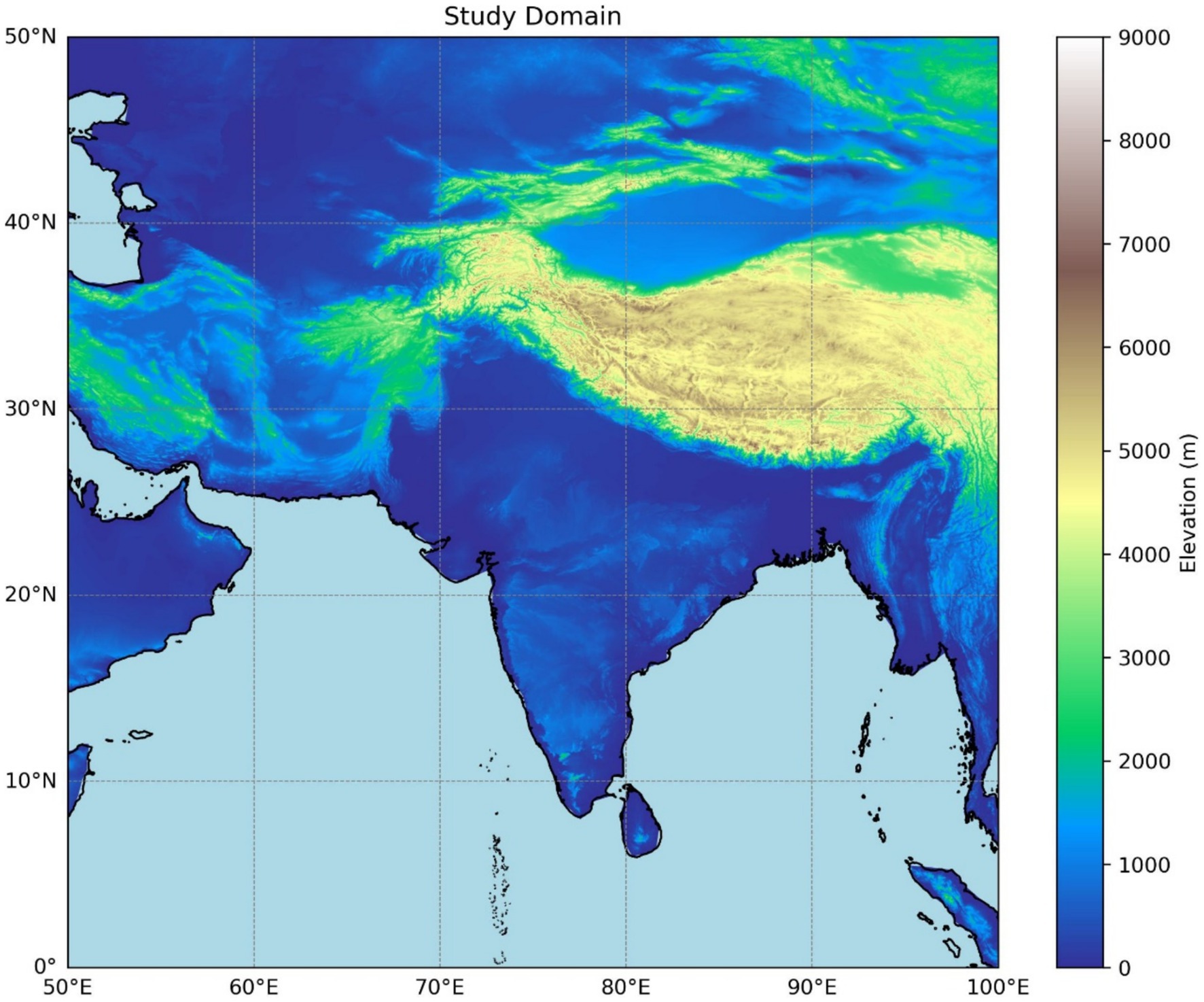
Figure 1. Study domain with the color bar representing the region’s elevation (in meters).
The 2-m temperature data from ERA5 from 1 January 1973 to 31 December 2023 are used; ERA5, the fifth-generation ECMWF reanalysis, offers comprehensive climate information from 1940 onward. It provides a detailed and consistent record of atmospheric, land, and oceanic parameters. The ERA5 dataset is known for its high spatial and temporal resolution, with 2-m hourly data available at a 0.25° × 0.25° grid. This high resolution makes ERA5 an invaluable resource for tasks such as downscaling, where high-precision data is crucial for accurate regional climate analysis. The dataset incorporates a vast array of observations and employs advanced data assimilation techniques, ensuring high accuracy and reliability in representing historical climate conditions. Using ERA5 data, this study benefits from the rich temporal coverage and detailed spatial granularity necessary for understanding and modeling temperature variations in the specified region.
3 Methodology
Three deep learning–based super-resolution techniques were applied to achieve a 10x downscaling of gridded 2-m temperature data. The three techniques are SRCNN, VDSR, and EDSR. All three downscaling methods use an end-to-end approach, which means that the networks do both the calibration and downscaling work simultaneously. The 51-year ERA5 hourly temperature dataset underwent data preprocessing steps described in Section 3.1. The convolutional layer utilizes filters that process the input data with a specified stride to extract spatial patterns. Each convolution operation was executed by calculating the element-wise dot product between the filters and various patches of the input. The outcome was optionally followed by a nonlinear transformation known as the activation function. This study employed the rectified linear unit (ReLU) activation function (He et al., 2016). The ReLU activation function is the most widely and extensively utilized activation function in hidden layers because of its efficiency and simplicity. Each model uses the same training, validation, and test sets. The downscaling methods’ training process is identical and follows a supervised learning approach. After a series of experiments, we found that it is best to train a network with a learning rate 0.0001. Therefore, for all the training cases, Adam optimizer with a learning rate of 0.0001 and MSE was used as the loss function, with a batch size of 16 was chosen as the common standard. SRCNN could run with a batch size up to 64, but EDSR encountered graphics processing unit (GPU) memory constraints at batch sizes above 16. To avoid overfitting, validation loss was calculated after every epoch. Finally, an evaluation is conducted on the three methods’ results using various metrics and explained in Section 3.3.
Most figures adopt perceptually uniform color palettes from the Scientific Color Maps (Crameri, 2018) collection. This has ensured that the figures’ color schemes are accessible to all readers with color vision deficiencies interpret our findings correctly.
3.1 Data preprocessing
The 2-m temperature data is divided into training (from 1 January 1973 to 31 December 2003), validation (from 1 January 2004 to 31 December 2013), and test (1 January 2014 to 31 December 2023) sets. The training set is utilized to calibrate the models, the validation set for optimization and mitigating overfitting, and the test set to assess the models’ efficacy on novel data. This configuration guarantees a thorough evaluation of the models’ capacity to generalize across various timeframes. We use the ERA5 2-m temperature data, initially available at an hourly resolution. The data was converted into daily mean temperature values by averaging the hourly data for each day to facilitate downscaling. The daily mean temperatures were calculated, yielding data at a spatial resolution of 0.25° × 0.25°. To train the downscaling models effectively, paired high-resolution and corresponding low-resolution datasets were necessary. Bilinear interpolation was applied to the high-resolution data, downsampling it to a spatial resolution of 2.5° × 2.5°. The low-resolution temperature data pairs, combined with the original high-resolution data, constituted the training dataset for the super-resolution and downscaling models. The low-resolution data functioned as input, whereas the high-resolution data served as the target output for model training, enabling models to learn to enhance low-resolution data and produce high-resolution outputs. All three downscaling methods require a data preprocessing step, which includes tasks such as normalization and resizing. Normalization is performed by subtracting the minimum value from each pixel and dividing by the range ([maximum value] − [minimum value]). This minimum–maximum normalization ensures that all the data values are within the range of [0, 1]. This improves the performance and convergence of the neural network. After the normalization process is performed as shown in (Equation 1), the normalized data is resized.
This normalization process uses to show the pixel intensity value in the image, min ( ) to show the lowest pixel intensity value, and max ( ) to show the highest pixel intensity value. This scaling changes each pixel to a value between 0 and 1. This keeps the relative intensities the same and improves consistency for analysis or training models. For resizing a Python-based library, OpenCV’s resize function is used to resize the data to a fixed image size. OpenCV (Open Source Computer Vision Library), originally developed by Intel® and now maintained by the OpenCV.org community (https://opencv.org). Consistent input data shape is vital for properly training neural networks. Finally, after the normalization and resizing are performed, all the preprocessed high- and low-resolution images are converted into NumPy arrays. This conversion to NumPy arrays was performed to ensure the efficient handling and processing by the neural network, and that it is in a suitable format for model training.
3.2 Downscaling methods
3.2.1 SRCNN
The Super-Resolution Convolutional Neural Network (SRCNN) (Figure 2) is designed to enhance image resolution through convolutional layers. It takes grayscale images as input, in our case, the temperature Network Common Data Form (NetCDF) file. We read and wrote gridded temperature data in Network Common Data Form (NetCDF), developed and maintained by the Unidata program at the University Corporation for Atmospheric Research (UCAR) (https://www.unidata.ucar.edu/software/netcdf), which was converted to NumPy arrays and will be treated as images by the networks. SRCNN consists of three primary layers: the first layer employs 64 filters with a 9 × 9 kernel, followed by a dimensionality-reducing layer with 32 filters and a 1 × 1 kernel. The final layer outputs the high-resolution image using a single filter with a 5 × 5 kernel. Compiled with the Adam optimizer at a learning rate of 0.0001 and using the Mean Squared Error (MSE) loss function. Our implementation of the SRCNN model includes minor modifications, which apply “same” padding. This step ensures the output dimensions remain the same as the input dimensions. We used the Adam optimizer instead of Stochastic Gradient Descent for faster convergence. SRCNN is effective for super-resolution tasks, making it suitable for medical imaging and satellite imagery applications.
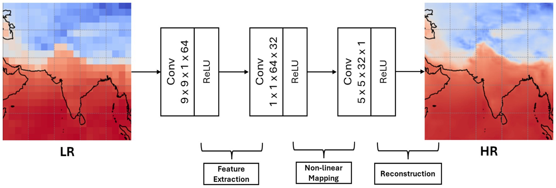
Figure 2. Illustration of the SRCNN model architecture that consists of three convolutional layers designed for super-resolution processing.
3.2.2 VDSR
The Very Deep Super-Resolution (VDSR) network (Figure 3) features a deep architecture comprising 20 convolutional layers, each utilizing 64 filters and 3 × 3 kernels with ReLU activation. This depth enables the model to capture intricate details essential for high-quality super-resolution. A residual learning approach is employed, adding the original input image to the output from the final layer, which helps alleviate the vanishing gradient problem. We implemented a VDSR model with slight modifications: utilizing the Adam optimizer with a learning rate of 0.0001, employing Keras’s default weight initialization. These modifications were implemented to enhance model performance and training stability within our application context. VDSR is optimized for effective training and high performance, making it suitable for tasks such as photography and satellite imagery.
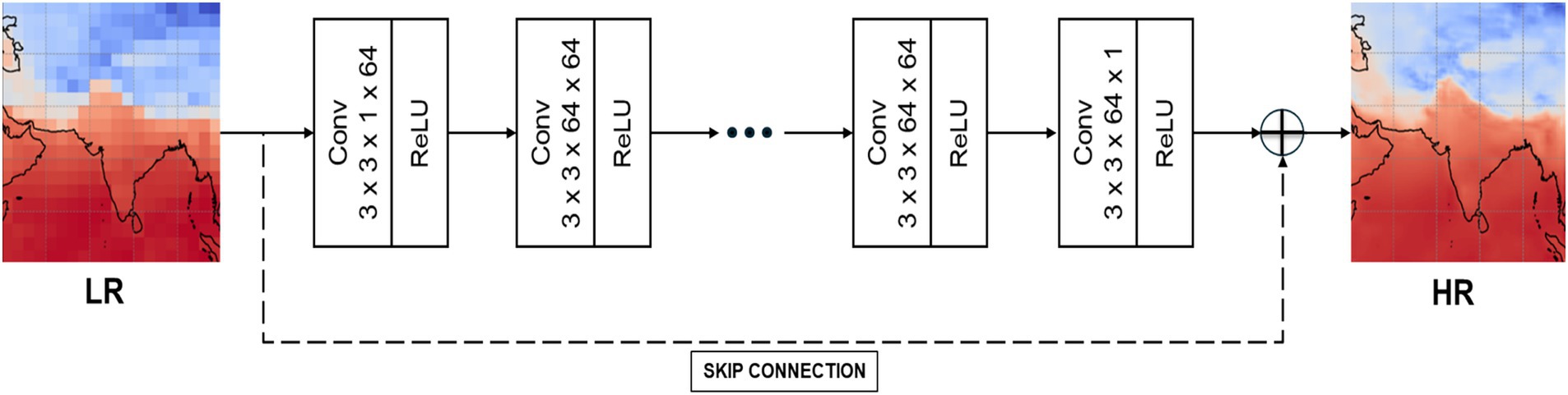
Figure 3. Illustration of the VDSR model architecture that consists of 20 convolutional layers and a single residual skip connection designed for super-resolution processing.
3.2.3 EDSR
The Enhanced Deep Super-Resolution (EDSR) model (Figure 4) is a state-of-the-art architecture that enhances image resolution through residual learning techniques. It features an input layer for grayscale images of size 201 × 201, an initial convolutional layer with 64 filters, and 16 residual blocks, each with two convolutional layers (Figure 5). The residual connections help mitigate vanishing gradient issues, enabling effective learning. The architecture concludes with a final convolutional layer and a residual addition, producing high-resolution output. Our implementation of the EDSR model incorporates slight modifications, that is, the exclusion of residual scaling and the utilization of grayscale input images. While based on the EDSR framework, these changes optimize the model for the specific application context of single-channel super-resolution. EDSR significantly improves image quality and detail, making it suitable for applications in photography and medical imaging.
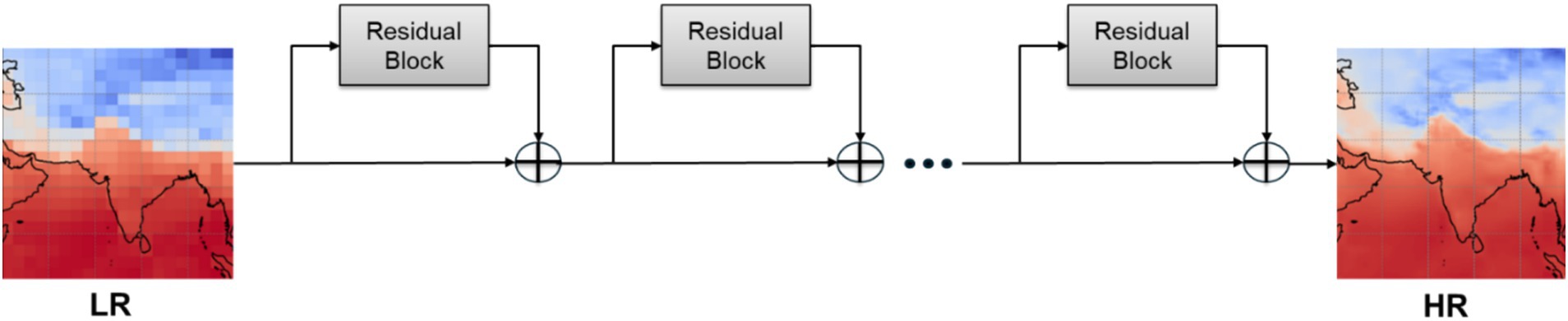
Figure 4. Illustration of the EDSR model architecture that includes 34 convolutional layers with 16 residual blocks.
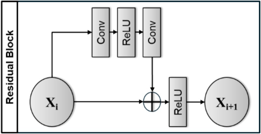
Figure 5. Residual Block in EDSR Model. A residual block in EDSR applies convolutional layers and ReLU activations, then adds the input to the output, producing . This skip connection aids in efficient learning.
3.3 Evaluation metrics
We employ two key metrics to assess the efficacy of downscaling models: Structural Similarity Index Measure (SSIM) and Peak Signal-to-Noise Ratio (PSNR). SSIM evaluates perceptual quality by analyzing luminance, contrast, and structural details between images, yielding a value ranging from −1 to 1, where values approaching 1 signify increased similarity. It is especially efficacious for assessing visual quality in tasks such as image reconstruction (Wang Z. et al., 2004). Additionally, we use multiscale-SSIM (MS-SSIM), which evaluates image quality at multiple scales. MS-SSIM captures both fine details and overall patterns, making it especially useful for climate data downscaling, where preserving small-scale features and global structure is critical. Unlike standard SSIM, MS-SSIM is more robust to local variations and noise, providing a more comprehensive assessment of model performance (Wang et al., 2003). PSNR, measured in decibels (dB), quantifies the ratio between the maximum signal and the accompanying noise, with elevated values indicating superior image fidelity (Huynh-Thu and Ghanbari, 2008). Both metrics are extensively utilized in image processing to assess the precision of generated outputs.
4 Results
4.1 Comparative analysis of downscaled temperature models
Accurately capturing temperature variations at a fine spatial scale in climate is critical for improving predictions and decision-making. We compare the performance of three deep learning-based super-resolution models—SRCNN, VDSR, and EDSR—in downscaling coarse-resolution ERA5 temperature data to a finer resolution of 0.25°. By comparing the outputs of these models, we can see how model complexity affects the accuracy and quality of temperature predictions, especially in regions with complex terrain such as the Himalayas. Here, visually comparing low-resolution and high-resolution temperature datasets can show how useful downscaling techniques are.
Figure 6 compares low-resolution ERA5 temperature data with downscaled outputs from three super-resolution deep learning models: SRCNN, EDSR, and VDSR, all at a resolution of 0.25°. The top-left plot presents the input low-resolution (2.5° × 2.5°) ERA5, exhibiting coarse temperature patterns with restricted spatial detail. The SRCNN output in the top-right considerably enhances resolution, improving visibility of local temperature variations, yet it remains imprecise in capturing finer details, particularly in mountainous regions. The bottom-right plot illustrates the VDSR model output, enhancing temperature gradients and accurately depicting local temperature variations, particularly in the regions affected by elevation and terrain, like the Himalayas. The bottom-left plot displays the EDSR output, providing the most precise and most detailed representation of temperature variations.
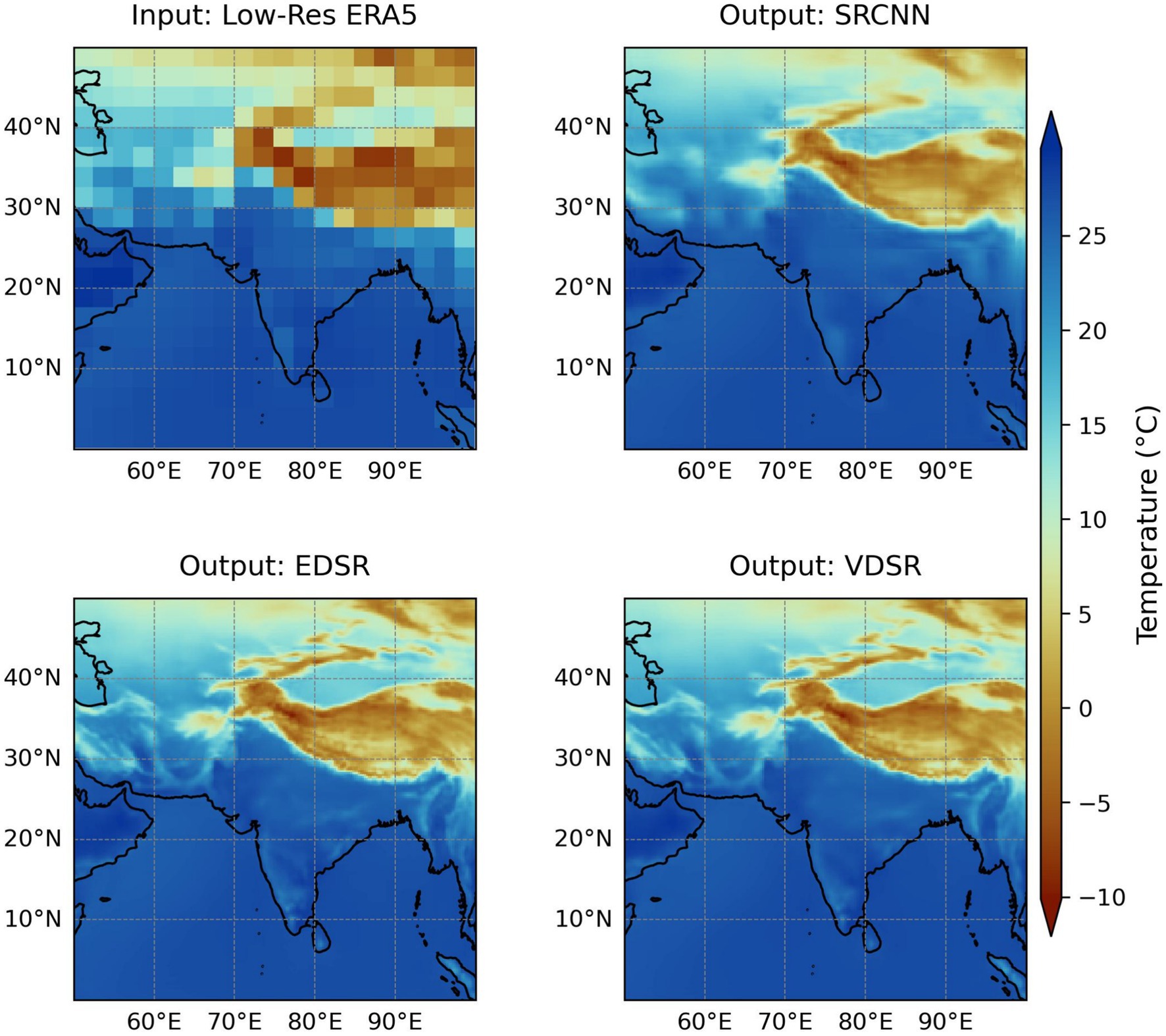
Figure 6. The first subplot shows the input 2.5° resolution ERA5 temperature data, while the other three subplots display the downscaled outputs generated using SRCNN, EDSR, and VDSR models, respectively, at 0.25° resolution.
4.2 Performance metrics and error threshold analysis across models
Table 1 presents a detailed comparison of the three super-resolution models (SRCNN, VDSR, and EDSR), emphasizing the escalating complexity and efficacy of each. SRCNN, comprising merely three convolutional layers and 8,129 trainable parameters, is the most rudimentary model and exhibits the poorest performance among the three, as indicated by structural similarity and image quality metrics, specifically SSIM (0.8466) and PSNR (28.65 dB). VDSR, comprising 20 layers and 665,921 parameters, employs just one residual connection to enhance depth, thereby capturing more complex details and markedly improving performance, attaining an SSIM of 0.9541 and a PSNR of 33.32 dB. The highly complex model, EDSR, comprising 34 layers and 1,219,841 parameters, significantly improves performance, attaining the highest SSIM (0.9629) and PSNR (34.01 dB). Considering that PSNR is a logarithmic metric, EDSR’s PSNR exceeds that of SRCNN by approximately 3.44 dB, signifying a significant enhancement in image quality. The inference performance and GPU memory utilization for the three super-resolution models are displayed in Table 1. SRCNN, the simplest model, shows moderate inference speed and minimal memory requirements. VDSR, due to its deeper architecture, offers marginally improved inference speed but requires greater peak memory consumption. EDSR, the most complex model, shows a slightly reduced inference speed and utilizes the most GPU memory. The results demonstrate the trade-off between improved image quality, resulting from greater model complexity, and the associated increase in computational resource demands.
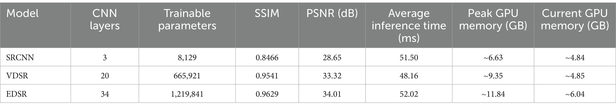
Table 1. Comparison of SRCNN, VDSR, and EDSR models, showing the number of CNN layers, trainable parameters, SSIM and PSNR values, along with their inference performance and GPU memory usage.
The effectiveness of the three super-resolution models (SRCNN, VDSR, and EDSR) on temperature data within different error thresholds is compared in Table 2. Thresholds at 1, 2, and 3°C show the percentage of predictions that fall inside these error ranges. SRCNN exhibits the lowest performance across all thresholds, with 38.84% of predictions accurate within 1°C, 68.04% within 2°C, and 78.81% within 3°C. VDSR achieves optimal performance at the 1°C error threshold, with 43.70% of predictions residing within that range. VDSR demonstrates enhancements at the 2 and 3°C thresholds, achieving 70.74 and 81.37% accuracy in predictions, respectively. EDSR demonstrates the highest accuracy at the 2 and 3°C thresholds, reaching 71.51 and 81.43% of predictions, respectively, while exhibiting a marginally lower performance at the 1°C threshold, with 39.00% of predictions within the margin.
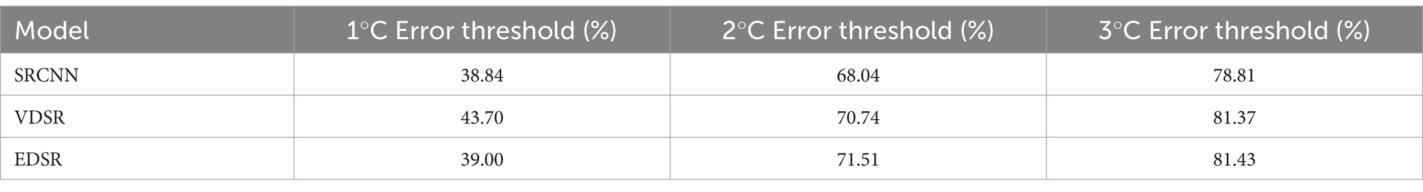
Table 2. This table shows the performance of SRCNN, VDSR, and EDSR models based on the percentage of predictions within 1, 2, and 3°C error thresholds.
4.3 Model comparison for the extreme temperature days
Figure 7 presents 12 subplots that illustrate the mean annual number of days during which temperature exceeds percentile thresholds of 90th, 95th, and 99th across the study region for the testing period (2014–2023). These subplots help assess the efficacy of the downscaled products in capturing the extreme temperature conditions associated with heat waves.
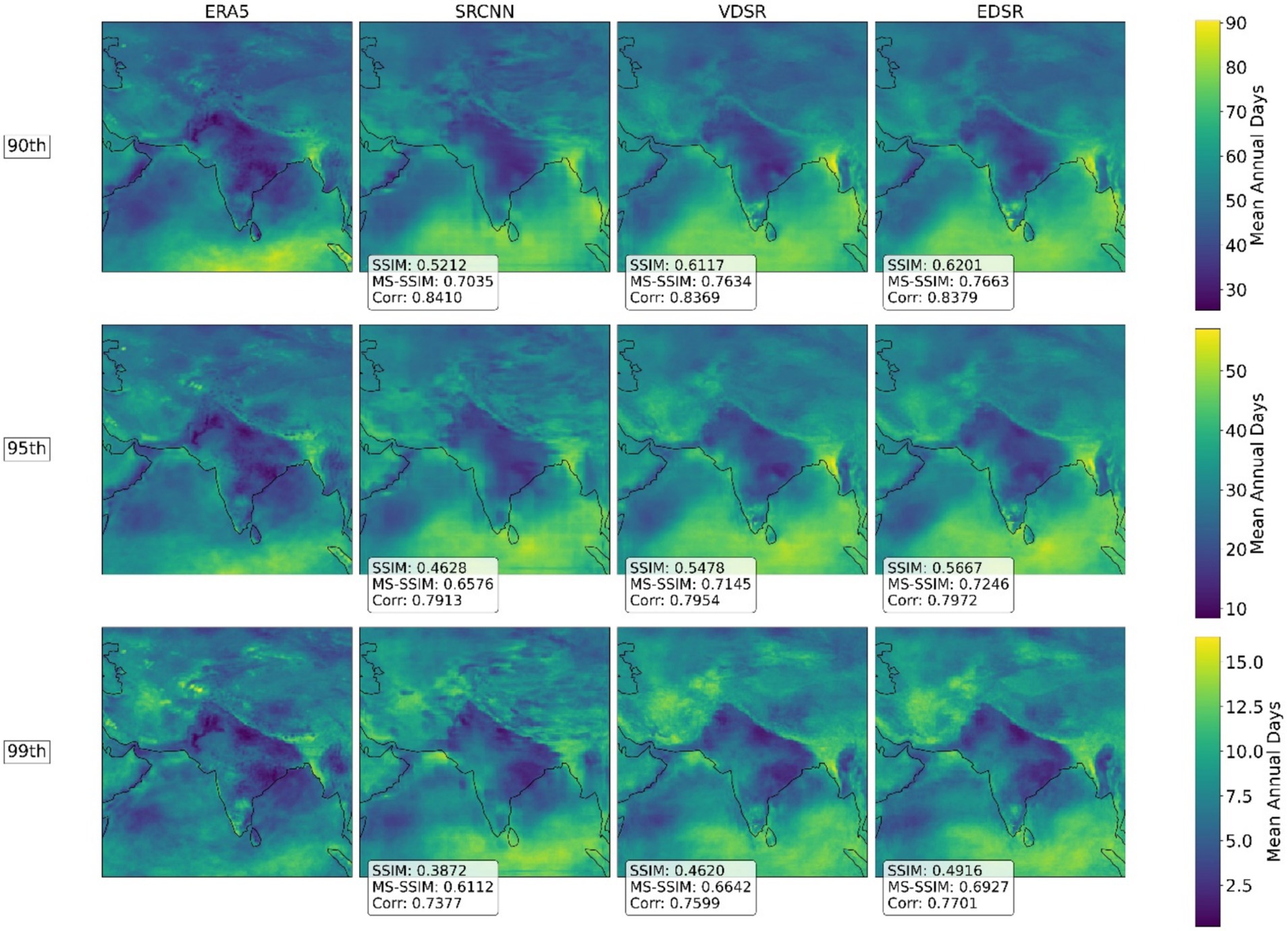
Figure 7. Comparison of mean annual exceedance days and performance metrics (SSIM, MS-SSIM, and pattern correlation) for ERA5 and deep learning models (SRCNN, VDSR, and EDSR) at the 90th, 95th, and 99th percentiles.
For each latitude–longitude grid cell, the 90th, 95th, and 99th percentiles were calculated using 51 years of daily temperature data and they were used as the threshold for plotting the mean annual number of days that the temperature at each grid cell exceeded these percentile thresholds (Klein Tank and Können, 2003; Data, 2009). In Figure 7. EDSR and VDSR consistently outperform the SRCNN across all metrics at all percentile thresholds. Percentile-based extreme event identification provides a more accurate representation across diverse climates, from the high mountains of the Himalayas and the Tibetan Plateau to the arid deserts of the Arabian Peninsula, rather than using a fixed threshold, like 30°C, established by the India Meteorological Department (IMD). Typically, climate data follows a baseline pattern, such as seasonal cycle or long-term trends, which are even somewhat captured by shallow networks. However, the extreme events, such as the exceedance of temperature from the 99th percentile, are best captured by the residual connections. Residual learning separates the predictable baseline from high-frequency anomalies, enabling the model to capture general climate trends and critical extreme events more effectively. The residual temperature maps presented in Figure 8 depict the discrepancies between the predicted temperatures from our three downscaling models (SRCNN, VDSR, and EDSR) and the observed ERA5 temperatures for the hottest day of 2023, which occurred on 22 July, with a mean temperature of 26.15°C for our study area. The analysis of the residual temperature maps indicates that SRCNN exhibits the poorest performance among all the models. SRCNN overestimates temperatures in the Himalayan mountains and Tibetan Plateau by 10–15°C; other models also exhibit this overestimation, albeit to a lesser extent than SRCNN. The overestimation is markedly diminished by utilizing residual learning in the downscaling method.
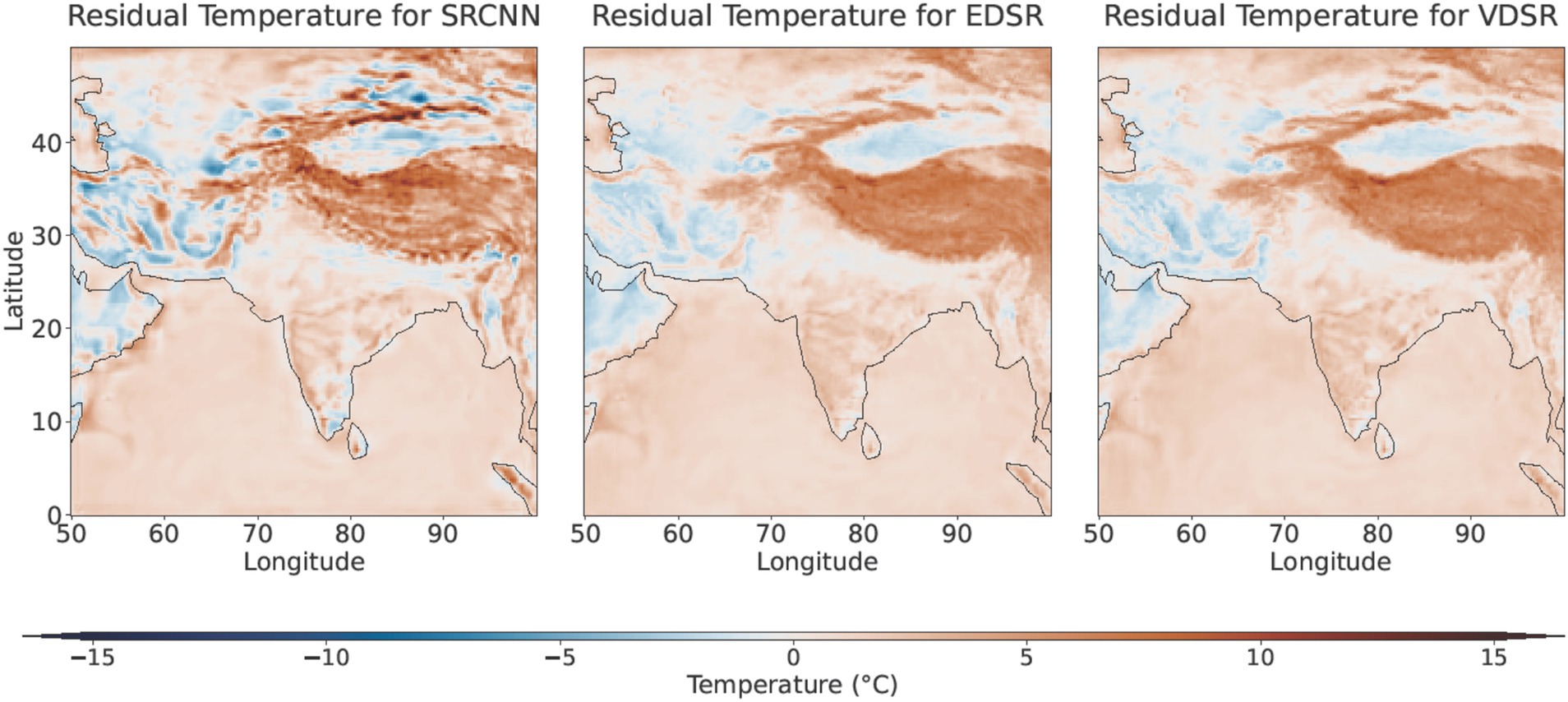
Figure 8. The residual temperature maps for 22 July 2023—the hottest day of that year—are presented for three models: SRCNN, EDSR, and VDSR. These maps illustrate the differences between the predicted and observed temperatures, highlighting each model’s performance in capturing temperature anomalies on that specific day.
In the SRCNN, several regions exhibited negative residuals ranging from 7 to 10°C; however, nearly all these areas disappeared in the residual maps produced by VDSR and EDSR. Similarly, Figure 9 illustrates the residual temperature map for the coldest day of 2023. The average temperature documented on 13 January was 6.89°C. Additionally, SRCNN’s map exhibits numerous locations where temperature estimations are both overestimated and underestimated, with a significant concentration of these locations along the Himalayan Mountain range and the Taklamakan Desert. Conversely, in downscaling methods based on residual learning, it is evident that these irregularities are significantly diminished. The residual learning-based models perform exceptionally well in mainland India, which exhibits relatively minimal topographical variations compared to the Himalayan regions. These models exhibit significantly smaller residuals, indicating more precise temperature predictions. The residual learning method effectively captures the accurate temperature distribution in simpler terrains, such as coastal areas and plains, where discrepancies between observed and predicted temperatures are minimal.
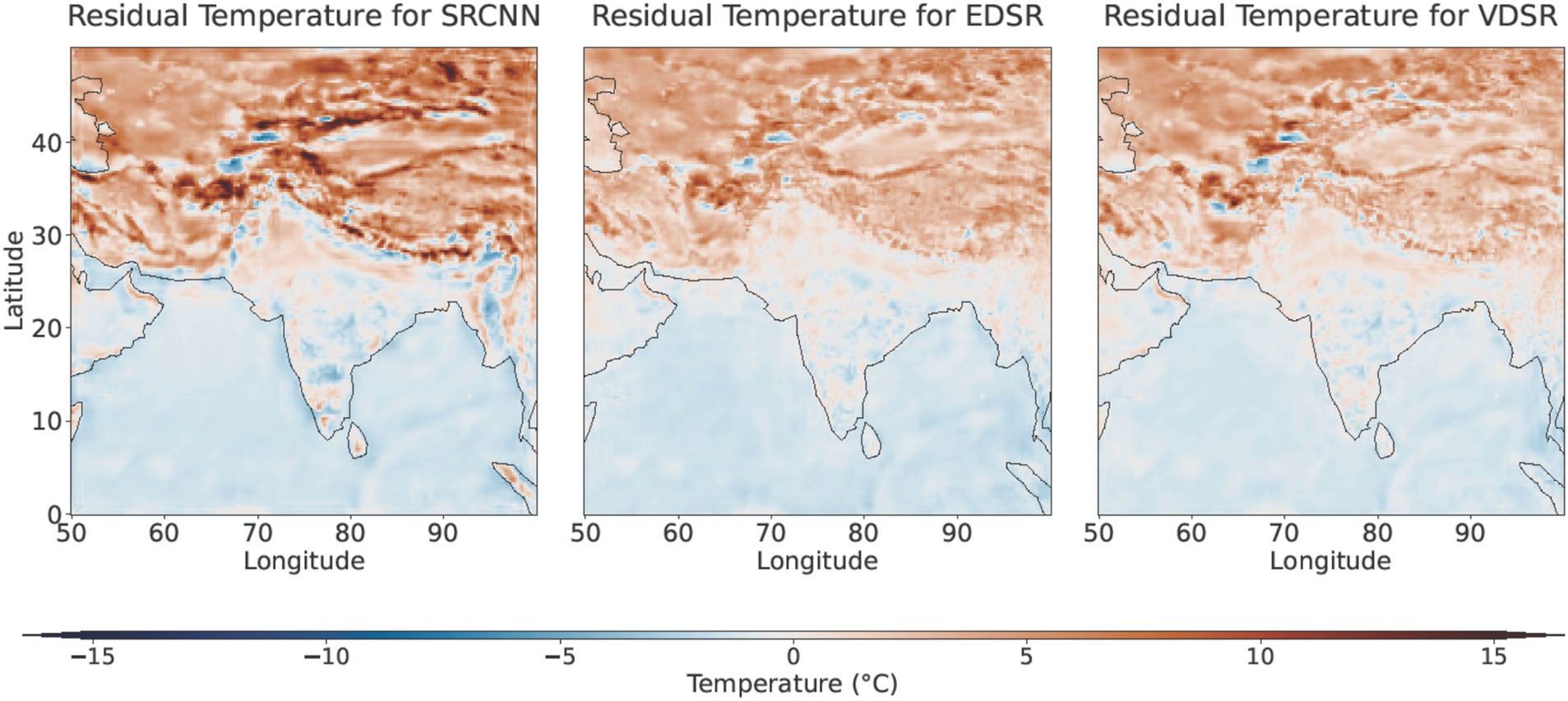
Figure 9. Residual temperature maps for the coldest day of 2023 (10 January), showing the differences between predicted and observed temperatures for the SRCNN, VDSR, and EDSR models.
4.4 Explainable AI techniques
Figure 10 reveals distinct spatial prioritization patterns based on saliency maps for all three downscaling models. The plots tell how each downscaling model architecture focuses during the downscaling performed by it. Here, SRCNN exhibits a narrow attention, concentrating exclusively on the Himalayan and the Tibetan regions. It is neglecting almost every critical location of the Indian subcontinent. The VDSR moderately expands this focus by incorporating adjacent zones beyond the Himalayan belt and Tibet. In contrast, EDSR demonstrates a comprehensive and diverse attention distribution throughout the Indian subcontinent. Apart from the mountainous regions, it also gives importance to the other parts, such as the hydrologically active Western Ghats, arid zones, and coastal belts. This expansive attention profile—enabled by EDSR’s residual learning framework—allows the model to integrate multiscale features across diverse terrains, preserving fine-grained details often lost in coarser architectures. The residual connections likely facilitate this by propagating contextual information through deeper layers, ensuring broader spatial awareness during downscaling. These results highlight that attention diversity is pivotal for capturing India’s geographic heterogeneity, directly translating to superior reconstruction fidelity in high-resolution 2-m temperature mapping.
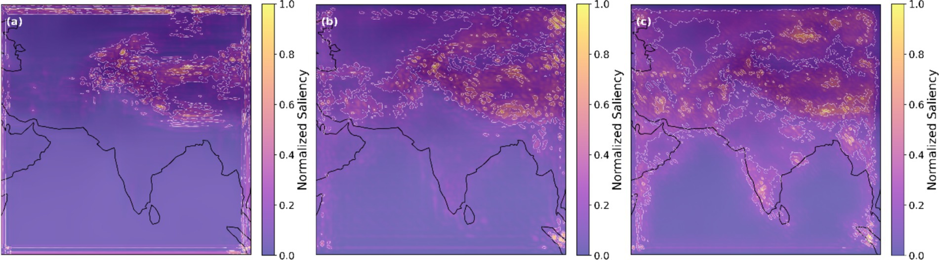
Figure 10. Saliency maps for (a) SRCNN, (b) VDSR, and (c) EDSR.
5 Discussion
5.1 Incompetencies with shallow CNNs in climate downscaling
Recent studies have assessed the efficacy of basic CNNs for downscaling 2-m temperature in comparison to traditional statistical downscaling techniques, revealing minimal enhancement (Baño-Medina et al., 2020; Miao et al., 2019; Pan et al., 2019; Lan et al., 2020; Vandal et al., 2019). Baño-Medina et al. (2020) evaluated CNN methodologies with three convolutional layers, SRCNN, and different configurations for downscaling temperature and precipitation in Europe. The results demonstrated overall enhancement; however, they were not consistently superior to traditional downscaling methods. Sun and Tang (2020) utilized the identical CNN methodology in China; however, their results were inferior to basic Bais Correction and Spatial Downscaling (BCSD) in accurately depicting temporal correlations, particularly concerning precipitation. Vandal et al. (2019) employed a three-convolutional layer SRCNN model to systematically downscale precipitation from a 1° resolution to a 0.125° resolution, applying a scaling ratio of 2 at each iteration, resulting in outcomes slightly better than the BCSD. The fundamental CNN architecture in previous deep learning downscaling consisted of only three convolutional layers, which is relatively shallow and may explain the limited improvement compared to conventional statistical downscaling methods. In contrast, the residual learning-based architecture was derived from an improved super-resolution CNN framework, consisting of more than 15 convolutional layers, which is considerably deeper than the previous simple CNN downscaling architecture (e.g., Baño-Medina et al., 2020; Pan et al., 2019; Vandal et al., 2019). Deep networks can seamlessly incorporate low, mid, and high-level features in an end-to-end multilayer manner. Research demonstrates that network depth is of critical importance (Simonyan and Zisserman, 2014). The findings have facilitated the broad application of extensive deep CNN architectures in multiple domains. We evaluated the benefits of the residual learning architecture by comparing it to the established three-layer convolutional plain architecture (SRCNN) for downscaling, in addition to the VDSR and EDSR architectures. Overall evaluations from metrics such as PSNR and SSIM indicate that VDSR and EDSR consistently surpass SRCNN in performance. For plain downscaling networks like SRCNN, model’s accuracy get saturated at a point and after that it degraded quickly with increase in number of layers that makes the model deeper (Wang and Tian, 2022).
5.2 Efficacy of advanced residual networks for climate data downscaling
Our comparison of three super-resolution models—SRCNN, VDSR, and EDSR—for downscaling temperature data offers valuable insights into the efficacy of various deep learning architectures. This discussion interprets the findings, focusing on the benefits of residual networks and the impact of architectural improvements such as depth and skip connections. The progression from SRCNN to VDSR and EDSR illustrates (Table 1) that increasing model complexity enhances the ability to capture fine details in climate data. This is evidenced by the significant improvements in super-resolution performance achieved through deeper architectures with residual connections, such as VDSR and EDSR, which effectively manage intricate patterns and spatial variations. The performance metrics across SSIM, PSNR, RMSE, and prediction accuracy at various temperature thresholds indicate that the residual networks (VDSR and EDSR) outperform the basic SRCNN model. According to the results of these two metrics shown in Table 2, we can say that residual networks-based models work better for the task of super-resolution, and EDSR is the best model for super-resolution. This superiority is attributed to the enhanced capacity of residual networks to capture complex patterns and fine details in the data. The residual learning framework, particularly in VDSR and EDSR, helps mitigate the degradation problem typically encountered in deeper networks by allowing the models to learn identity mappings, thereby focusing on refining the residuals between the high- and low-resolution data. Efficient training of deeper networks is possible with residual connections. The risk of overfitting and vanishing gradient is also absent, which allows capturing more complex temporal and spatial dependencies. With these skip connections there is more effective backpropagation hence these networks learn complex mappings which are inherent in climate data (Wang et al., 2024). EDSR emerges as the best-performing model in terms of SSIM and PSNR, showcasing its ability to produce high-quality, structurally accurate images. Its architectural refinement, primarily removing unnecessary batch normalization layers and increasing depth, enhances its capacity to reconstruct high-resolution details effectively. The improved performance of EDSR in broader error allowances (2°C and 3°C thresholds) further emphasizes its robustness and generalization capabilities. VDSR, while slightly lagging behind EDSR in structural similarity and image quality, demonstrates the highest precision within the 1°C error threshold. This indicates its proficiency in making precise predictions, which can be crucial for applications requiring high accuracy in localized temperature estimates. The deeper architecture of VDSR, coupled with residual learning, enables it to capture intricate patterns, leading to lower RMSE and MAE values than SRCNN. Its focus on wider activation functions and deeper networks allows it to balance performance and computational efficiency, making it a viable option for practical applications where resources are constrained. The capability of EDSR to identify nuanced local patterns, especially in complex topographies, highlights the advantages of deeper residual networks for climate data downscaling. The plots shown in Figure 6 demonstrate that EDSR and VDSR surpass SRCNN, yielding more precise and detailed temperature representations at higher resolutions. However, with the improved accuracy achieved by these residual connection-based networks, they come with trade-offs, that is, an increase in computational resources. These improvements in the downscaling can also be achieved for other variables such as precipitation and wind speed, few studies have used residual connections in some ways and have achieved better results—to name a few: Sharma and Mitra (2022), Wang and Tian (2022), Wang et al. (2021), Liu et al. (2020), and Wang et al. (2024).
5.3 Residual patterns and model efficiency across climatic zones
Figures 11, 12 illustrate average temperature maps for the validation period (2004–2013) and the testing period (2014–2023). The maps illustrate the residuals (the difference between predicted and actual values) from three distinct downscaling models: SRCNN, VDSR, and EDSR throughout South Asia. SRCNN encounters difficulties in areas with complex topography, such as the Himalayas, likely due to the complexities of temperature predictions influenced by elevation and microclimate factors. This region exhibits notable orange and red streaks, signifying a persistent overestimation of temperature over the 20-year period from 2004 to 2023. EDSR and VDSR demonstrate a reduced presence of orange and red streaks, indicating diminished overestimation in predictions derived from the residual network compared to SRCNN. It also shows that they are managing the high-altitude regions of Tibet and the Himalayan belt more effectively. Significant enhancements are evident in the areas of Iran and Afghanistan, as SRCNN exhibits considerable inconsistency in certain parts of this region. The SRCNN both underestimates and overestimates in various areas of this region, indicating its failure to downscale in arid to semi-arid climates effectively. The challenge of maintaining consistent temperature predictions in arid climates is addressed by the residual learning models VDSR and EDSR. Both models exhibit significantly superior performance in these areas, demonstrating minimal residuals compared to SRCNN. Over the Indian Ocean, all three models perform exceptionally well. Both validation (Figure 11) and testing (Figure 12) show very low residuals across most of the region, likely because of the low temperature variability over the ocean. However, residuals are higher along the coastal boundaries, where land meets sea, especially for SRCNN, while VDSR and EDSR maintain lower errors. This suggests that the advanced residual network architectures (VDSR and EDSR) are more effective at capturing subtle variations in these challenging transition zones, further supporting their superior overall performance in downscaling applications.
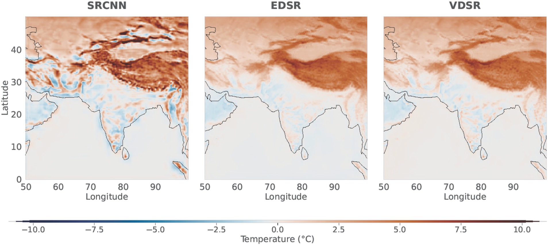
Figure 11. Mean residual temperature maps representing the differences between predicted and observed temperatures for the validation period 2004–2013.
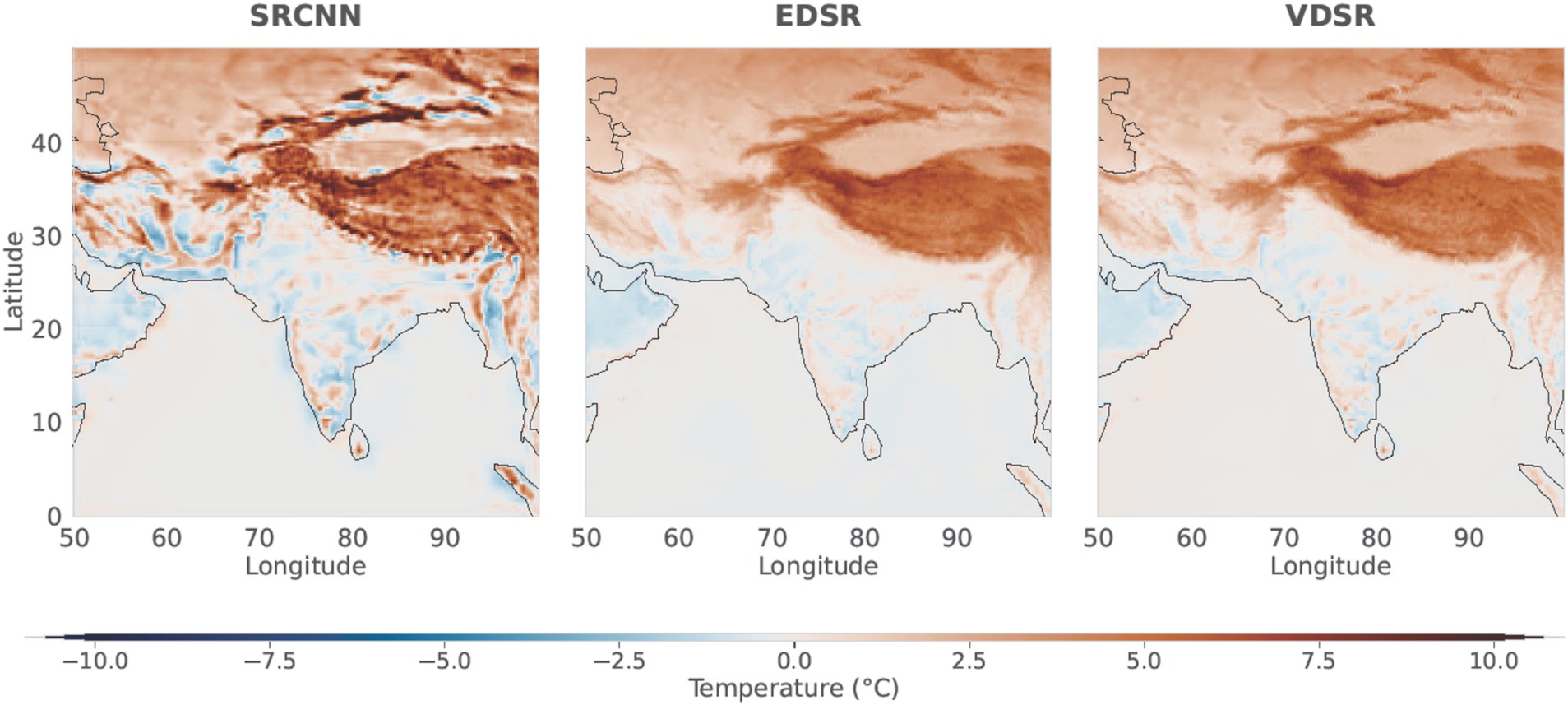
Figure 12. Mean residual temperature for the testing period 2014–2023.
The plots in Figure 13 demonstrate each model’s ability to reduce error. These threshold map plots indicate the percentage of the region where the models’ temperature predictions fall below 1, 2, and 3°C. The plots illustrate the precision of each model, indicating that as the error tolerance rises (from 1 to 3°C), the proportion of areas with model predictions within the acceptable error range also increases. At a threshold of 1°C, all models exhibit subpar performance; however, predictions based on residual learning consistently surpass those of SRCNN. Notably, we observe a substantial enhancement in arid climatic regions of Pakistan, Afghanistan, and Iran. Additionally, certain areas of southern India exhibit improvements in prediction. At 2 and 3°C errors, the hue of blue intensifies, indicating an increasing number of points falling within the threshold from 2014 to 2023. Despite a relaxed error threshold of 3°C, a persistent white region is evident in the Himalayas and the Tibetan Plateau, an extensive high-altitude region encompassing northern India, Nepal, Bhutan, and Western China. The difficulty in accurately predicting temperatures in these regions likely arises from the intricate terrain and severe conditions, where models fail to capture the complex climate variations effectively. Upon increasing the error threshold to 3°C, the white regions diminish slightly in size, yet they remain considerable. The enduring white regions indicate where the models encounter difficulties.
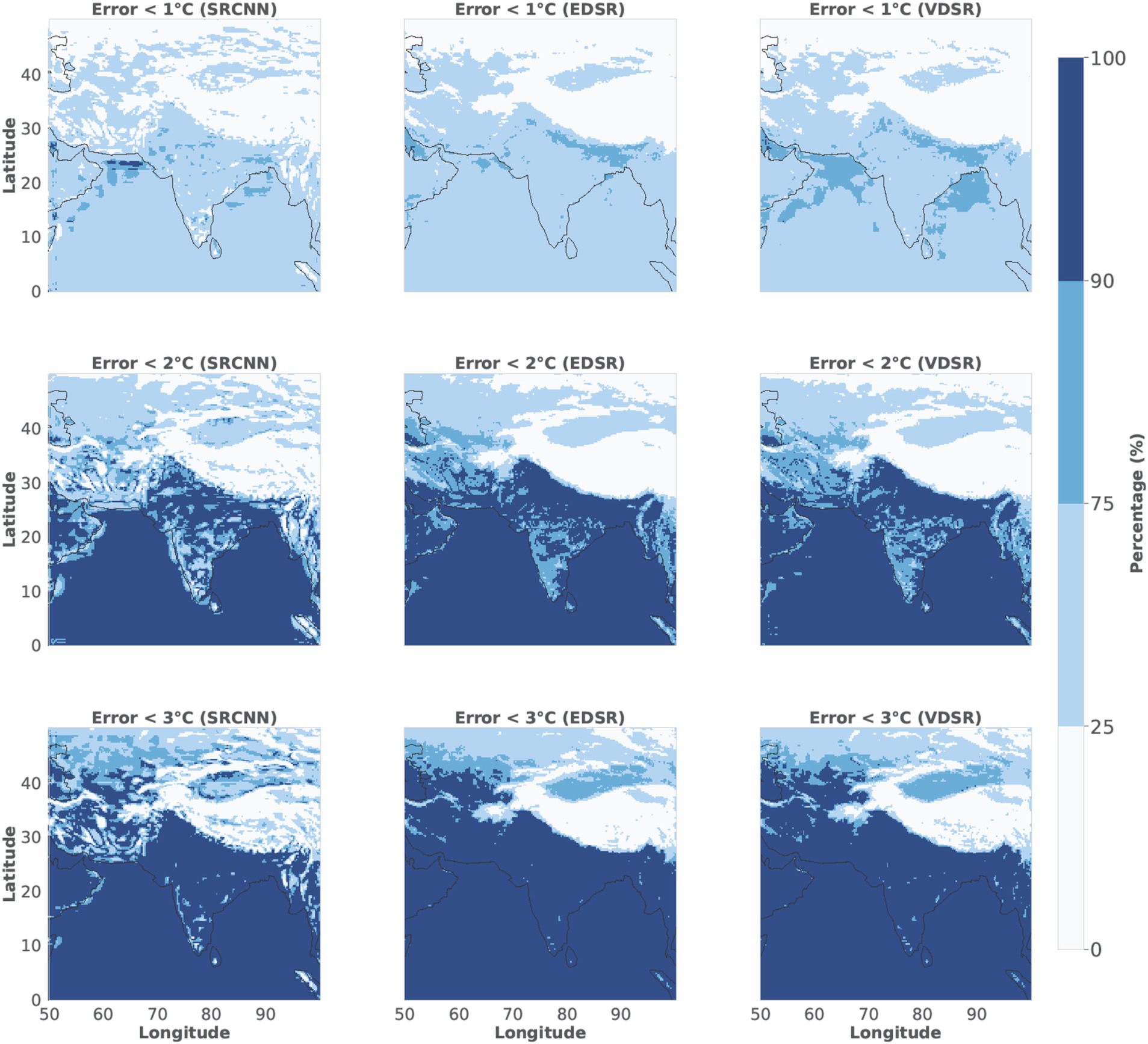
Figure 13. Illustrations of the threshold map plots for each model (SRCNN, VDSR, and EDSR) indicate the percentage of regions where temperature predictions fall within 1, 2, and 3°C thresholds. Each model is shown for the period 2014–2023, with varying error tolerance levels.
5.4 Limitations and potential areas for further research
Despite the promising results, several limitations persist; notably, the deep learning-based downscaling models fail to predict temperature in complex climatic regions, such as high-altitude regions of the Himalayas and the Tibetan Plateau; another region that remains a problem is the arid to semi-arid region of Afghanistan and Iran. These problems must be addressed so that our downscaling results are more comprehensive. One way to do this is by including additional variables; for example, elevation information would improve the downscaling results in the Himalayas and the Tibetan Plateau, or the addition of climatic variables such as precipitation, humidity, and wind speed can improve the predictions in arid to semi-arid climatic zones. Our current study focuses on deterministic downscaling using a deep learning model approach and not the uncertainty quantification, which we recognize is crucial for climate downscaling. In future research, we will extend this work to incorporate probabilistic output methods such as the Monte Carlo dropout and ensemble model approaches. This will help address the uncertainty and further enhance the downscaled outputs. XAI also has its limitations, as shown by a few studies, it was inconsistent with conclusions from different XAI techniques (Rudin et al., 2019). Some inherent issues are related to the nature of XAI (Bommer et al., 2023). XAI results must be interpreted carefully as they tend to oversimplify the decision-making process of the DL-based downscaling models. Recently, a few researchers have started exploring the use of XAI in the field of climate science (Mamalakis et al., 2022). In the future work, we plan to integrate physics-informed constraints and compare critical thermodynamic variables (e.g., lapse rates and energy fluxes) between the downscaled outputs and independent observations to ensure that the results maintain fidelity with established atmospheric dynamics. We plan to explore physics-informed neural networks to incorporate atmospheric dynamics and thermodynamic constraints into our downscaling framework.
6 Conclusion
The study examines three super-resolution models (SRCNN, VDSR, and EDSR) for downscaling temperature data ranging approximately from 250 km to 25 km spatial resolution. It focuses on the benefits of residual networks and architectural improvements such as depth and skip connections. The results conclusively demonstrate that residual networks, particularly VDSR and EDSR, significantly outperform the baseline SRCNN model in terms of SSIM, PSNR, RMSE, MAE, and predictive accuracy. As shown by VDSR and EDSR, increasing the network depth makes it easier for the model to figure out complex structural features from the data. This makes it easier to see how temperatures change in places with complicated terrain, such as the Himalayas, the Tibetan Plateau, and Afghanistan’s semi-arid areas. With an SSIM of 0.9629 and a PSNR of 33.88 dB, EDSR has the best overall performance, showing that it can reconstruct images very well. However, VDSR also does much better, with an SSIM of 0.9729 and a PSNR of 32.92 dB, especially for assessing localized temperature. This approach of incorporating residual connections effectively identified local extreme events (Figure 7) and demonstrated significant potential for precise downscaling in the absence of local-scale data. In addition, adding skip connections greatly improves the performance and training efficiency of these residual networks by reducing the vanishing gradient problem. This makes it easier to train deeper architectures. The study shows that both VDSR and EDSR are better than SRCNN across all error ranges (1, 2, and 3°C) based on temperature thresholds, with EDSR doing better across wider thresholds and VDSR doing better within the 1°C error margin. In agriculture, water resource management, and urban planning, where precise temperature data is essential, enhancements in prediction accuracy in these areas are vital. Even though the models have some benefits, none of them can consistently make predictions within 3°C in places such as the Tibetan Plateau, where temperature patterns change quickly and make it hard to make accurate predictions. This limitation shows the importance of including extra elevation data in the downscaling process to make the model more accurate in rough terrain. Adding additional data, such as humidity or rainfall, may also make the model work better in dry areas. The results show that residual-based deep learning models could help make climate models more accurate, especially in places with different landscapes and weather conditions. By making better temperature predictions, these models are useful tools for fields such as agriculture, urban planning, and water resource management that need accurate temperature predictions. In the future, researchers might investigate applying residual networks to other climate variables and regions to see how well they work on a larger scale and in more challenging conditions. This would help us understand climate impacts and how to reduce them better.
Data availability statement
Data related to this article is publicly available from ERA5 (https://cds.climate.copernicus.eu/datasets/reanalysis-era5-single-levels?tab=overview).
Author contributions
SJh: Conceptualization, Data curation, Formal analysis, Investigation, Methodology, Software, Validation, Visualization, Writing – original draft, Writing – review & editing. VG: Conceptualization, Methodology, Project administration, Resources, Supervision, Validation, Writing – review & editing. PS: Writing – review & editing. AM: Writing – review & editing. SJo: Writing – review & editing.
Funding
The author(s) declare that financial support was received for the research and/or publication of this article. This research was supported by the Department of Space, Government of India, under the Research Sponsored (RESPOND) program of the Indian Space Research Organisation (ISRO) [grant number: DS-2B-13012(2)/17/2025-Sec.2].
Conflict of interest
The authors declare that the research was conducted in the absence of any commercial or financial relationships that could be construed as a potential conflict of interest.
Generative AI statement
The authors declare that Generative AI was used in the creation of this manuscript. The author(s) utilized ChatGPT ((Natural-language processing was assisted by ChatGPT, a large-language model developed by OpenAI.) and QuillBot (QuillBot, proprietary software provided by QuillBot, Inc. (https://quillbot.com).) to improve the manuscript’s readability and language during its preparation. After using these tools, the author(s) evaluated and revised the content as necessary and assume full responsibility for the published article’s content.
Publisher’s note
All claims expressed in this article are solely those of the authors and do not necessarily represent those of their affiliated organizations, or those of the publisher, the editors and the reviewers. Any product that may be evaluated in this article, or claim that may be made by its manufacturer, is not guaranteed or endorsed by the publisher.
References
Allen, J. T. (2018). Climate change and severe thunderstorms. In H. Storchvon (Ed.) Oxford research encyclopdia of climate science, Oxford University Press, New York.
Asrar, G., and Dozier, J. (1994). EOS Science Strategy for the Earth Observing System. Woodbury, New York: American Institute of Physics Press.
Balmaceda-Huarte, R., Baño-Medina, J., Olmo, M. E., and Bettolli, M. L. (2024). On the use of convolutional neural networks for downscaling daily temperatures over southern South America in a climate change scenario. Clim. Dyn. 62, 383–397.
Baño-Medina, J., Manzanas, R., and Gutiérrez, J. M. (2020). Configuration and inter-comparison of deep learning neural models for statistical downscaling. Geosci. Model Dev. 13, 2109–2124. doi: 10.5194/gmd-13-2109-2020
Baño-Medina, J., Manzanas, R., and Gutiérrez, J. M. (2021). On the suitability of deep convolutional neural networks for continental-wide downscaling of climate change projections. Clim. Dyn. 57, 2941–2951. doi: 10.1007/s00382-021-05847-0
Barbhuiya, S., Manekar, A., and Ramadas, M. (2024). Performance evaluation of ML techniques in hydrologic studies: comparing streamflow simulated by SWAT, GR4J, and state-of-the-art ML-based models. J. Earth Syst. Sci. 133:136. doi: 10.1007/s12040-024-02340-0
Bellard, C., Bertelsmeier, C., Leadley, P., Thuiller, W., and Courchamp, F. (2012). Impacts of climate change on the future of biodiversity. Ecol. Lett. 15, 365–377. doi: 10.1111/j.1461-0248.2011.01736.x
Bilal, S. B., and Gupta, V. (2024). Deciphering the spatial fingerprint of drought propagation through precipitation, vegetation and groundwater. Int. J. Climatol. 44, 4443–4461. doi: 10.1002/joc.8590
Bommer, P., Kretschmer, M., Hedstroem, A., Bareeva, D., and Hoehne, M. M. C. (2023). Evaluation of explainable AI solutions in climate science. In EGU General Assembly Conference Abstracts (pp. EGU-12528).
Christensen, J. H., Hewitson, B., Busuioc, A., Chen, A., Gao, X., Held, I., et al. (2007). “Regional climate projections” in Climate Change 2007: the physical science basis. Contribution of Working Group I to the Fourth Assessment Report of the Intergovernmental Panel on Climate Change. eds. S. Solomon, D. Qin, M. Manning, Z. Chen, M. Marquis, and K. B. Averyt (Cambridge: Cambridge University Press).
Crameri, F. (2018). Geodynamic diagnostics, scientific visualisation and StagLab 3.0. Geosci. Model Dev. 11, 2541–2562. doi: 10.5194/gmd-11-2541-2018
Data, C. (2009). Guidelines on analysis of extremes in a changing climate in support of informed decisions for adaptation. Geneva: World Meteorological Organization.
Dee, D. P., Uppala, S. M., Simmons, A. J., Berrisford, P., Poli, P., Kobayashi, S., et al. (2011). The ERA-interim reanalysis: configuration and performance of the data assimilation system. Q. J. R. Meteorol. Soc. 137, 553–597. doi: 10.1002/qj.828
Fox-Kemper, B. (2021). “Ocean, cryosphere and sea level change” in Climate Change 2021: The Physical Science Basis. Contribution of Working Group I to the Sixth Assessment Report of the Intergovernmental Panel on Climate Change. eds. V. P. Masson-Delmotte, A. Zhai, S. L. Pirani, C. Connors, and S. Péan (Cambridge: Cambridge University Press).
Frame, D. J., Rosier, S. M., Noy, I., Harrington, L. J., Carey-Smith, T., Sparrow, S. N., et al. (2020). Climate change attribution and the economic costs of ex-treme weather events: a study on damages from extreme rainfall and drought. Clim. Chang. 162, 781–797. doi: 10.1007/s10584-020-02729-y
Giorgi, F. (2006). Climate change hot-spots. Geophys. Res. Lett. 33:25734. doi: 10.1029/2006GL025734
González‐Abad, J., Baño‐Medina, J., and Gutiérrez, J. M. (2023). Using explainability to inform statistical downscaling based on deep learning beyond standard validation approaches. J. Adv. Model. Earth Syst. 15:e2023MS003641.
Goodfellow, I., Pouget-Abadie, J., Mirza, M., Xu, B., Warde-Farley, D., Ozair, S., et al. (2020). Generative adversarial networks. Commun. ACM 63, 139–144. doi: 10.1145/3422622
Gosling, S. N., and Arnell, N. W. (2016). A global assessment of the impact of climate change on water scarcity. Clim. Chang. 134, 371–385. doi: 10.1007/s10584-013-0853-x
Guo, Y., Liu, Y., Oerlemans, A., Lao, S., Wu, S., and Lew, M. S. (2016). Deep learning for visual understanding: a review. Neurocomputing 187, 27–48. doi: 10.1016/j.neucom.2015.09.116
Gupta, V., and Jain, M. K. (2020). Impact of ENSO, global warming, and land surface elevation on extreme precipitation in India. J. Hydrol. Eng. 25:05019032. doi: 10.1061/(ASCE)HE.1943-5584.0001872
Gupta, V., Syed, B., Pathania, A., Raaj, S., Nanda, A., Awasthi, S., et al. (2024). Hydrometeorological analysis of July-2023 floods in Himachal Pradesh, India. Nat. Hazards 120, 1–26. doi: 10.1007/s11069-024-06520-5
Hansen, J., Sato, M., Ruedy, R., Lo, K., Lea, D. W., and Medina-Elizade, M. (2006). Global temperature change. Proc. Natl. Acad. Sci. 103, 14288–14293. doi: 10.1073/pnas.0606291103
He, K., Zhang, X., Ren, S., and Sun, J. (2016). Deep residual learning for image recognition. In Proceedings of the IEEE conference on computer vision and pattern recognition IEEE: Las Vegas. (pp. 770–778).
Held, I. M., Guo, H., Adcroft, A., Dunne, J. P., Horowitz, L. W., Krasting, J., et al. (2019). Structure and performance of GFDL's CM4. 0 climate model. J. Adv. Model. Earth Syst. 11, 3691–3727. doi: 10.1029/2019MS001829
Hersbach, H., Bell, B., Berrisford, P., Hirahara, S., Horányi, A., Muñoz-Sabater, J., et al. (2020). The ERA5 global reanalysis. Q. J. R. Meteorol. Soc. 146, 1999–2049. doi: 10.1002/qj.3803
Hewitson, B. C., and Crane, R. G. (1996). Climate downscaling: techniques and application. Clim. Res. 7, 85–95. doi: 10.3354/cr007085
Hughes, T. P., Kerry, J. T., Álvarez-Noriega, M., Álvarez-Romero, J. G., Anderson, K. D., Baird, A. H., et al. (2017). Global warming and recurrent mass bleaching of corals. Nature 543, 373–377. doi: 10.1038/nature21707
Huynh-Thu, Q., and Ghanbari, M. (2008). Scope of validity of PSNR in image/video quality assessment. Electron. Lett. 44, 800–801. doi: 10.1049/el:20080522
IPCC (2021). Climate Change 2021: The physical science basis. Working Group I Contribution to the IPCC Sixth Assessment Report. Cambridge: Cambridge University Press.
Justice, C. O., Townshend, J. R. G., Vermote, E. F., Masuoka, E., Wolfe, R. E., Saleous, N., et al. (2002). An overview of MODIS land data pro-cessing and product status. Remote Sens. Environ. 83, 3–15. doi: 10.1016/S0034-4257(02)00084-6
Kalnay, E. (1996). The NCEP/NCAR 40-year reanalysis project. Bull. Am. Meteorol. Soc. 77, 437–471. doi: 10.1175/1520-0477(1996)077<0437:TNYRP>2.0.CO;2
Kim, J., Lee, J. K., and Lee, K. M. (2016). Accurate image super-resolution using very deep convolutional networks. In Proceedings of the IEEE conference on computer vision and pattern recognition IEEE: Las Vegas, NV, (pp. 1646–1654).
Klein Tank, A. M. G., and Können, G. P. (2003). Trends in indices of daily temperature and precipitation extremes in Europe, 1946–99. J. Clim. 16, 3665–3680. doi: 10.1175/1520-0442(2003)016<3665:TIIODT>2.0.CO;2
Lan, R., Sun, L., Liu, Z., Lu, H., Su, Z., Pang, C., et al. (2020). Cascading and enhanced residual networks for accurate single-image super-resolution. IEEE Trans. Cyber. 51, 115–125. doi: 10.1109/TCYB.2019.2952710
LeCun, Y., Bengio, Y., and Hinton, G. (2015). Deep learning. Nature 521, 436–444. doi: 10.1038/nature14539
Lim, B., Son, S., Kim, H., Nah, S., and Mu Lee, K. (2017). Enhanced deep residual networks for single image super-resolution. In Proceedings of the IEEE conference on computer vision and pattern recognition workshops. IEEE: Honolulu, HI (pp. 136–144).
Liu, Y., Ganguly, A. R., and Dy, J. (2020). Climate downscaling using YNet: a deep convolutional network with skip connections and fusion. In Proceedings of the 26th ACM SIGKDD international conference on Knowledge Discovery & Data Mining Association for Computing Machinery, New York (pp. 3145–3153).
Lobell, D. B., Schlenker, W., and Costa-Roberts, J. (2011). Climate trends and global crop production since 1980. Science 333, 616–620. doi: 10.1126/science.1204531
Mamalakis, A., Barnes, E. A., and Ebert-Uphoff, I. (2022). Investigating the fidelity of explainable artificial intelligence methods for applications of convolutional neural networks in geoscience. Artif. Intell. Earth Syst. 1:e220012.
Maraun, D. (2013). Bias correction, quantile mapping, and downscaling: revisiting the inflation issue. J. Clim. 26, 2137–2143. doi: 10.1175/JCLI-D-12-00821.1
McMichael, A. J., Woodruff, R. E., and Hales, S. (2006). Climate change and human health: present and future risks. Lancet 367, 859–869. doi: 10.1016/S0140-6736(06)68079-3
Miao, Q., Pan, B., Wang, H., Hsu, K., and Sorooshian, S. (2019). Improving monsoon precipitation prediction using combined convolutional and long short term memory neural network. Water 11:977. doi: 10.3390/w11050977
Nicholls, R. J., and Cazenave, A. (2010). Sea-level rise and its impact on coastal zones. Science 328, 1517–1520. doi: 10.1126/science.1185782
Pan, B., Hsu, K., AghaKouchak, A., and Sorooshian, S. (2019). Improving precipitation estimation using convolutional neural network. Water Resour. Res. 55, 2301–2321. doi: 10.1029/2018WR024090
Pathania, A., and Gupta, V. (2024). Beyond the extremes: Interpretable insights based on Attention framework (No. EGU24-14818). Vienna, Austria: EGU General Assembly.
Pecl, G. T., Araújo, M. B., Bell, J. D., Blanchard, J., Bonebrake, T. C., Chen, I. C., et al. (2017). Biodiversity redistribution under climate change: Impacts on ecosystems and human well-being. Science, 355:eaai9214.
Pendergrass, A. G., and Knutti, R. (2018). The uneven nature of daily precipitation and its change. Geophys. Res. Lett. 45, 11–980. doi: 10.1029/2018GL080298
Raaj, S., Gupta, V., Singh, V., and Shukla, D. P. (2024). A novel framework for peak flow estimation in the himalayan river basin by integrating SWAT model with machine learning based approach. Earth Sci. Inf. 17, 211–226. doi: 10.1007/s12145-023-01163-9
Rampal, N., Gibson, P. B., Sood, A., Stuart, S., Fauchereau, N. C., Brandolino, C., et al. (2022a). High-resolution downscaling with interpretable deep learning: rainfall extremes over New Zealand. Weather Clim. Extr. 38:100525. doi: 10.1016/j.wace.2022.100525
Rampal, N., Shand, T., Wooler, A., and Rautenbach, C. (2022b). Interpretable deep learning applied to rip current detection and localization. Remote Sens. 14:6048. doi: 10.3390/rs14236048
Reichstein, M., Camps-Valls, G., Stevens, B., Jung, M., Denzler, J., Carvalhais, N., et al. (2019). Deep learning and process understanding for data-driven earth system science. Nature 566, 195–204. doi: 10.1038/s41586-019-0912-1
Rienecker, M. M., Suarez, M. J., Gelaro, R., Todling, R., Bacmeister, J., Liu, E., et al. (2011). MERRA: NASA’s modern-era retrospective analysis for research and applications. J. Clim. 24, 3624–3648. doi: 10.1175/JCLI-D-11-00015.1
Rosenzweig, C., Elliott, J., Deryng, D., Ruane, A. C., Müller, C., Arneth, A., et al. (2014). Assessing agricultural risks of climate change in the 21st century in a global gridded crop model intercomparison. Proc. Natl. Acad. Sci. 111, 3268–3273. doi: 10.1073/pnas.1222463110
Rudin, C. (2019). Stop explaining black box machine learning models for high stakes decisions and use interpretable models instead. Nat. Mach. Intell. 1, 206–215.
Saha, S., Moorthi, S., Pan, H. L., Wu, X., Wang, J., Nadiga, S., et al. (2010). The NCEP climate forecast system reanalysis. Bull. Am. Meteorol. Soc. 91, 1015–1058. doi: 10.1175/2010BAMS3001.1
Samset, B. H., Zhou, C., Fuglestvedt, J. S., Lund, M. T., Marotzke, J., and Zelinka, M. D. (2023). Steady global surface warming from 1973 to 2022 but increased warming rate after 1990. Commun. Earth Environ. 4:400. doi: 10.1038/s43247-023-01061-4
Schär, C., Vidale, P. L., Lüthi, D., Frei, C., Häberli, C., Liniger, M. A., et al. (2004). The role of increasing temperature variability in European summer heatwaves. Nature 427, 332–336. doi: 10.1038/nature02300
Scott, T., Masselink, G., O'Hare, T., Saulter, A., Poate, T., Russell, P., et al. (2016). The extreme 2013/2014 winter storms: beach recovery along the southwest coast of England. Mar. Geol. 382, 224–241. doi: 10.1016/j.margeo.2016.10.011
Seneviratne, S., Nicholls, N., Easterling, D., Goodess, C., Kanae, S., Kossin, J., et al. (2012). “Changes in climate extremes and their impacts on the natural physical environment” in Managing the risks of extreme events and disasters to advance climate change adaptation. eds. C. B. Field, V. Barros, T. F. Stocker, and Q. Dahe (Cambridge: Cambridge University Press).
Sharma, S. C. M., and Mitra, A. (2022). ResDeepD: a residual super-resolution network for deep downscaling of daily precipitation over India. Environ. Data Sci. 1:e19. doi: 10.1017/eds.2022.23
Shen, C. (2018). A transdisciplinary review of deep learning research and its relevance for water resources scientists. Water Resour. Res. 54, 8558–8593. doi: 10.1029/2018WR022643
Simonyan, K., and Zisserman, A. (2014). Very deep convolutional networks for large-scale image recognition. arXiv preprint arXiv:1409.1556.
Stirling, I., and Derocher, A. E. (2012). Effects of climate warming on polar bears: a review of the evidence. Glob. Chang. Biol. 18, 2694–2706. doi: 10.1111/j.1365-2486.2012.02753.x
Sun, A. Y., and Tang, G. (2020). Downscaling satellite and reanalysis precipitation products using attention-based deep convolutional neural nets. Front. Water 2:536743. doi: 10.3389/frwa.2020.536743
Urban, M. C. (2015). Accelerating extinction risk from climate change. Science 348, 571–573. doi: 10.1126/science.aaa4984
Vandal, T., Kodra, E., and Ganguly, A. R. (2019). Intercomparison of machine learning methods for statistical downscaling: the case of daily and extreme precipitation. Theor. Appl. Climatol. 137, 557–570. doi: 10.1007/s00704-018-2613-3
Wang, Z., Bovik, A. C., Sheikh, H. R., and Simoncelli, E. P. (2004). Image quality assessment: from error visibility to structural similarity. IEEE Trans. Image Process. 13, 600–612. doi: 10.1109/TIP.2003.819861
Wang, Y., Leung, L. R., McGREGOR, J. L., Lee, D. K., Wang, W. C., Ding, Y., et al. (2004). Regional climate modeling: progress, challenges, and prospects. J. Meteorol. Soc. Jpn. 82, 1599–1628. doi: 10.2151/jmsj.82.1599
Wang, L., Li, Q., Peng, X., and Lv, Q. (2024). A temporal downscaling model for gridded geophysical data with enhanced residual U-net. Remote Sens. 16:442. doi: 10.3390/rs16030442
Wang, Z., Simoncelli, E. P., and Bovik, A. C. (2003). Multiscale structural similarity for image quality assessment. In The Thrity-seventh Asilomar conference on signals, systems & computers, 2003 (1398–1402). IEEE: Pacific Grove, CA.
Wang, F., and Tian, D. (2022). On deep learning-based bias correction and downscaling of multiple climate models simulations. Clim. Dyn. 59, 3451–3468. doi: 10.1007/s00382-022-06277-2
Wang, F., Tian, D., Lowe, L., Kalin, L., and Lehrter, J. (2021). Deep learning for daily precipitation and temperature downscaling. Water Resour. Res. 57:e2020WR029308. doi: 10.1029/2020WR029308
Watts, N., Adger, W. N., Agnolucci, P., Blackstock, J., Byass, P., Cai, W., et al. (2015). Health and climate change: policy responses to protect public health. Lancet 386, 1861–1914. doi: 10.1016/S0140-6736(15)60854-6
Wheeler, T., and Von Braun, J. (2013). Climate change impacts on global food security. Science 341, 508–513. doi: 10.1126/science.1239402
Wilby, R. L., and Dawson, C. W. (2013). The statistical downscaling model: insights from one decade of application. Int. J. Climatol. 33, 1707–1719. doi: 10.1002/joc.3544
Wilby, R. L., and Wigley, T. M. (1997). Downscaling general circulation model output: a review of methods and limitations. Prog. Phys. Geogr. 21, 530–548. doi: 10.1177/030913339702100403
Keywords: downscaling, deep learning, temperature, residual networks, ERA5, climate change, explainable AI
Citation: Jha SK, Gupta V, Sharma PJ, Mishra A and Joshi S (2025) Deep learning super-resolution for temperature data downscaling: a comprehensive study using residual networks. Front. Clim. 7:1572428. doi: 10.3389/fclim.2025.1572428
Edited by:
Vikram Kumar, Planning and Development, Govt. of Bihar, IndiaReviewed by:
Detelina Ivanova, Climformatics Inc., United StatesAbhishek Banerjee, Chinese Academy of Sciences (CAS), China
Copyright © 2025 Jha, Gupta, Sharma, Mishra and Joshi. This is an open-access article distributed under the terms of the Creative Commons Attribution License (CC BY). The use, distribution or reproduction in other forums is permitted, provided the original author(s) and the copyright owner(s) are credited and that the original publication in this journal is cited, in accordance with accepted academic practice. No use, distribution or reproduction is permitted which does not comply with these terms.
*Correspondence: Vivek Gupta, dml2ZWtndXB0YUBpaXRtYW5kaS5hYy5pbg==