A review on principles, performance and complexity of linear estimation and detection techniques for MIMO systems

The advent of the fifth generation (5G) of mobile networks has introduced several new use cases that are pushing mobile networks in environments that are typically supported by wired technologies. The initial discussions around the sixth generation (6G) of mobile networks signalizes that different approaches are needed to address all contrasting requirements, where multiple-input multiple-output (MIMO) technique stands as a key technology for most future wireless systems. In this review, we present an introduction on classical linear estimators and coherent detectors along with an innovative and accurate complexity formulation within a common framework, allowing a fair comparison and providing an initial guideline for researchers that are looking for a general view of the main techniques available for spatial multiplexing (SM)-MIMO detection and estimation.

1 Introduction

Since the first generation (1G) of mobile communication in the 1980s until today, the field of digital communication has tremendously evolved both in capacity and reliability (Giordani et al., 2020). The emerging fifth generation (5G) is driving mobile communication systems towards an unprecedented evolution in terms of flexibility, data rate and latency, enabling wireless networks to support applications that are typically backed by wired technologies. The scenarios for the sixth generation (6G) are even harder to achieve considering the foreseen increase in flexibility, while supporting conflicting requirements for several applications in different verticals, besides higher data rates, higher coverage, higher frequency bands and extreme low latency. It is clear that future mobile networks cannot rely on a single radio access network to fulfill all these requirements. Different approaches are needed to address all requirements, but multiple-input multiple-output (MIMO) schemes represent a key technology for most future wireless systems. For example, in the agribusiness scenario, high data rates are necessary to transmit multi-spectral videos in infrared, ultraviolet and visible light in real time from drone to the cloud. In industry 4.0, very low latency is necessary for controlling robots and synchronizing autonomous actions with humans on the plant floor. MIMO can provide the necessary bandwidth, reducing the frame duration and increasing the robustness for data with a very short life span. Communication systems employing MIMO techniques present significant advantages when compared with traditional SISO architectures, i.e., mitigating fading effects by creating spatial diversity or exploiting channel scattering to achieve higher data rates by spatial multiplexing means. MIMO systems with detection schemes that can harvest diversity and multiplexing gains are able to improve the throughput, increase coverage and reduce the outage probability at the same time. Although the mentioned advantages are appealing features in the future mobile communication context, they are accompanied by demanding drawbacks such as uncorrelated transmission channels requirement, in order to avoid weak conditioned channel matrices, high signaling coordination on MIMO channel estimation, considering each individual transmitting antenna and higher complexity for the network nodes. The challenges imposed by the mobile communication channels require complex processes on the receiver side to recover the information with a desired quality of service (QoS). Among these processes, the estimation and detection algorithms tailored for mobile communications deserve special attention, since the interest on these techniques is growing constantly with the adoption of new schemes, such as MIMO, reconfigurable intelligent surfaces (RIS) (Tapio et al., 2021) and new waveforms (Zhang et al., 2017).

In the digital communications context, the estimation process is associated with choosing a hypothesis from an uncountable infinite set of hypotheses, according to some predefined criteria. One interesting example in communication systems is the channel estimation, where an estimate of the channel impulse response or the channel frequency response must be obtained on the receiver side with minimal mean-squared error (MSE). On the other hand, the detection procedure relates to making a decision from a countably finite set of hypotheses following, again, some established criterion. Another interesting example in the digital communication system is the discrete data detection. In this case, the detector must decide in favor of one of the M possible data symbols from a discrete sample space (or constellation) using the maximum likelihood or the minimum distance criteria (Gallager, 2008). The detectors and estimators analyzed in this paper are used to recover data in the downlink of mobile networks, where the base station (BS) and the user equipment (UE) employ orthogonal frequency division multiplexing (OFDM) with multiple transmit and receive antennas for space multiplexing. The channel is assumed to be frequency-selective and time-variant, with coherence time larger than the symbol block length and coherence bandwidth larger than one subcarrier.

Since these topics are widely studied, the number of different techniques available in the literature can be overwhelming. Hence, this paper aims for presenting an introduction on two critical tasks of mobile communication physical layer (PHY), which are: a) the linear estimation algorithms, suitable for channel state information (CSI) estimation and equalization and; b) detection and non-linear estimators schemes, in order to surpass the limitations of linear estimators in certain applications, i.e., spatial multiplexing (SM)-MIMO (Foschini, 1996). The analysis of beamforming MIMO and non-coherent detectors are beyond the scope of this intro work and can be addressed in (Ahmed et al., 2018; Mahmoud and El-Mahdy, 2021) for the interested reader. Other studies are also available in the literature as follows.

An extensive survey on detection algorithms related to massive MIMO can be found in (Albreem et al., 2019), where well-known linear detectors, including linear equalizers and suitable iterative methods as alternatives to avoid matrix inversion, are characterized according to its performance and complexity profiles. This reference also chronologically lists pertinent publications on MIMO subject. Similarly, in (Albreem et al., 2021a), low complexity linear detectors employing different numerical solutions for the large matrix inversion problem are evaluated, comparing its respective estimated computational cost and resource utilization in a system level deployment.

Still related to this topic, a recent overview on precoding techniques for massive MIMO is conducted (Albreem et al., 2021b). The idea behind precoding is to simplify the detection task on the receiver terminal, transferring its complexity to the transmission side, at the BS, which is in charge of precoding the transmitted information, employing suitable and eventually heavy digital pre-processing. This work also lists features, advantages, challenges and research opportunities related to massive MIMO. Moreover, it discusses and summarizes different precoding algorithms such as linear and non-linear precoders, RIS based precoder and machine learning deep neural network precoding. It concludes that, although linear precoders suffer from performance deterioration under certain scenarios, they still play a crucial role in the transmitter design due to their relative simplicity. This conclusion reinforces the importance of linear estimation concepts discussed here.

In (Jang et al., 2021; Pereira de Figueiredo, 2022), machine learning is pointed out as an important enabling technology for applications such as MIMO, massive MIMO and beamspace MIMO in the millimeter wave. It is notable that machine learning is gathering special attention from the academic community thanks to its potential to replace statistical driven solvers by generalist and adaptive learning-based techniques. Machine learning based MIMO detectors can even outperform the classic approaches when the channel statistical behavior does not match the model considered in the design of the model-driven detectors. Crucial tasks as channel estimation and detection (Ye et al., 2018), resource management (Hussain et al., 2020) and other optimization problems (Dahrouj et al., 2021) are being revisited under the machine learning perspective and, undoubtedly, will play an important role in 6G (Kaur et al., 2021; Sarkar and Debnath, 2021).

An accessible overview encompassing the state-of-the-art solutions to the detection problem is available in (Larsson, 2009). Prominent linear equalizers and detectors are investigated in (Kobayashi et al., 2014), presenting bit error rate (BER) performance analysis and computational complexity comparison under the assumption of different channel correlation scenarios.

In (Jalden and Ottersten, 2005), the sphere detector (SD) is examined, presenting the respective complexity in terms of the number of visited nodes, culminating in the definition of lower and upper bounds for the computational cost given the channel matrix dimension, constellation size and signal-to-noise ratio (SNR).

In this review article, regarding estimators and equalizers, we concentrate in the linear minimum mean squared error (LMMSE) estimator and its low cost iterative variances (Sayed, 2003; Proakis, 2007) as feasible alternatives to address the large matrix inversion problem. Moreover, the component-wise conditionally unbiased (CWCU)-LMMSE (Lang and Huemer, 2015) is considered as an appropriate equalization method featured by an additional weighting process leading to a constrained unbiased estimation. We also present detailed derivations for these estimators and its respective MSE, allowing the reader to investigate the estimation error performance along the Bayesian Cramer-Rao bound (BCRB) as a an absolute reference. Besides this analysis, computational complexity is formulated and further evaluated, seeking to identify which techniques present reasonable performance and affordable computational cost.

Regarding the detector, we focus on the renowned and relevant detection methods for the spatial multiplexing multiple-input multiple-output (SM-MIMO) applications, encompassing the Maximum Likelihood Detector (MLD), the minimum mean squared error (MMSE)- ordering successive interference cancellation (OSIC) (Hampton, 2013), the SD (Hassibi and Vikalo, 2005) and the iterative MMSE- Parallel Interference Cancellation (PIC) detector (Bensaad et al., 2013), presenting a compiled reviewing about these techniques together with each algorithm description. Furthermore, respective computational cost is derived, allowing one to conduct a complexity comparison alongside a performance analysis through a Monte Carlo BER simulation.

One of the main contributions of this tutorial work relies on.

• gathering and compiling the principles of classical estimators and detectors, in a uniform and accessible way, supported by detailed description of the procedures of each analyzed technique;

• performing a complexity comparison among the techniques in terms of float-point operations (FLOPs) under a common framework, allowing a fairly analysis and providing an interesting reference for researchers starting in this field.

In order to achieve these goals, the remaining of this manuscript is structured as follows: Section 2 presents a simplified model to linearly describe a generic and orthogonal digital communication PHY that will be used as a reference along this paper. Section 3 brings the background on complexity analysis of algorithms employed in estimation and detection problems. In Sections 4 and Sections 5, in this order, we present the main techniques for linear estimation and detection, their derivations, and estimated complexity. Section 6 presents numerical examples and performance analysis of the techniques described in Sections 4 and Sections 5, but tailored to specific applications on low order SM-MIMO, such as equalization and detection. Finally, Section 7 presents the conclusions by highlighting the main findings and results achieved in this paper.

Notation: Matrices and vectors are written in boldface uppercase and lowercase as X and x, respectively. A random variable observation is represented as a sub-indexed lowercase x_i. The notation $\mathsf{E}\{\cdot \}$ is the expected value of a given random entity. The exponent (⋅)^H is the transpose and conjugate (Hermitian) operator. The mean and the covariance of a given random vector, e.g. x, are defined as ${\mathit{\mu }}_{\mathbf{x}}=\mathsf{E}\{\mathbf{x}\}$ and ${\mathbf{C}}_{\mathbf{x}\mathbf{x}}=\mathsf{E}\{\mathbf{x}{\mathbf{x}}^{\mathrm{H}}\}-\mathsf{E}\{\mathbf{x}\}\mathsf{E}{\{\mathbf{x}\}}^{\mathrm{H}},$ respectively. The operator diag (⋅) gives the diagonal of a square matrix or, when the argument is a vector, it returns a square matrix whose diagonal is populated with the vector elements. The symbol ∇_α,βf(x) represents the differentiation of the function f(x) with respect to α and β. The Frobenius norm of a generic matrix A is defined by ‖A‖² ≜∑_i,j∣A_ij∣², with A_ij being the elements of matrix A. The set of real and complex numbers are denoted by ${\mathbb{R}}^{m\times n}$ and ${\mathbb{C}}^{m\times n}$, respectively, where m and n are the dimension size of the numerical structure.

2 System model for the digital communication PHY

This section introduces the concept of an orthogonal multicarrier digital communication PHY as a linear model, which is employed in following sections of this paper.

In a broad sense, a digital communication PHY is responsible for: a) adapting the digital information to a waveform that is transmitted to one or more receivers through a communication channel, and; b) for retrieving the information on the receiver side from the distorted and noisy version of the transmitted signal. Both transmitter and receiver are designed based on the communication channel characteristics as noise and fading statistics, average scattering pattern, coherence time, coherence bandwidth and the impairments introduced by the transmitter’s and receiver’s RF front-end, among others. Specifically for a modern mobile communication system, the PHY must deal with double-dispersive MIMO channels, where each path between one transmitting and one receiving antenna is modeled as a time-variant and frequency-selective impulse response. We consider a scheme employing n transmitting antennas and m receiving antennas as a generalization of the mobile communication system, as it embraces more simplified arrangements, e.g., the usual soft-input soft-output (SISO) when m = n = 1. It is worth to mention that, assuming a SM-MIMO case, when m = n ≥ 2, inter-antenna interference (IAI) takes place once each receiving antenna might collect signals from more than one transmitting antennas. In this case, the detection method should be carefully chosen to take the trade-off between performance and complexity into account. Figure 1 illustrates a simplified wireless communication system assuming this scenario.At the transmitter side, the Bit Encoding block receives the data bit sequences and protects them by applying randomization, forward error correction (FEC) (Ryan and Lin, 2009) and interleaving, aiming to increase the system robustness against the adverse effects of the mobile channel. The resulting coded bits are then fed to the Waveform Modulator block, where different techniques may be used, e.g., symbol modulation and multicarrier techniques, leading to specific waveforms tailored for mobile MIMO channels. The channel block introduces time and frequency fading and it combines the transmitted signals at each receiving antenna, besides adding the additive white Gaussian noise (AWGN). On the receiver side, the Waveform Demodulation block is responsible for performing the time and frequency synchronization, waveform demodulation, antenna decoupling and data symbol estimation, while the Bit Decoding block is responsible for correcting the bit errors that might be introduced by the channel. In SISO iterative detection, the Bit Decoding performs soft demapping in order to obtain soft coded bit sequences, in the form of Log-Likelihood Ratios (LLRs), carrying a sort of confidence measurement about the bit sequence. The LLRs are fed backwards to Waveform Demodulation block as a-priori information, subscripted $\widehat{b}$ in Figure 1, leading to a more refined symbol estimation at each iteration. After an appropriate number of iterations, the bit information is decided from decoded LLRs. In non-iterative detection, the Bit Decoding block directly decodes the bit sequences once. The recovered binary sequence is finally delivered for the data sink (user application).

FIGURE 1

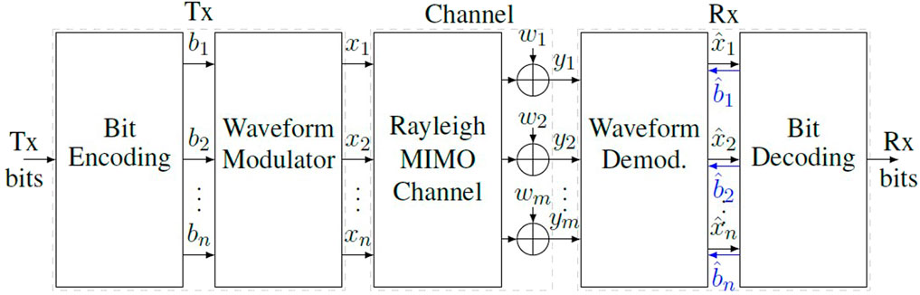
FIGURE 1. Simplified block diagram of a generic and communication system.

It is worth to clarify that, despite of its importance in the communication research field, the availability of studies involving channel coding techniques are wide and easily found in literature, thus, beyond the scope of this work. Instead, this work relies on available algorithms in (Glavieux and Vaton, 2007; Ryan and Lin, 2009), such as Convolutional Codes (CCs) and A-Posteriori Probability (APP) decoding.

Next, we describe the matricial notation for the orthogonal multicarrier MIMO, since this scheme is one of the most popular solution for the air interface in mobile communication systems.

2.1 Orthogonal multicarrier MIMO PHY

Consider the system from Figure 1, where n × m antennas may be employed, resulting in n × m paths between the transmitter and receiver. The channel impulse response (CIR) between the jth transmitting antenna and the ith receiving antenna with L taps is represented by ${\tilde{\mathbf{h}}}_{i,j}\in {\mathbb{C}}^{L\times 1}$.

Assuming that an uncoded and non-precoded OFDM is employed as multi-carrier modulation scheme to transmit n parallel streams of N_s Quadrature Amplitude Modulation (QAM) symbols, mapped into K_on active subcarriers from a total of K. Let ${\bar{\mathbf{x}}}_j\in {\mathbb{C}}^{K\times 1}$ be the data vector in frequency domain transmitted by the jth transmitting antenna with j = 1, 2, …, n and K_on ≤ K. The transmitted samples is obtained performing an inverse discrete Fourier transform (DFT), leading to

${\mathit{\chi }}_j={\mathbf{F}}_K^{\mathrm{H}}{\bar{\mathbf{x}}}_j.(1)$

where ${\mathbf{F}}_K\in {\mathbb{C}}^{K\times K}$ is the unitary Fourier matrix. In order to protect the transmit samples ${\mathit{\chi }}_j\in {\mathbb{C}}^{K\times 1}$ against the intersymbol interference (ISI) introduced by a dispersing channel, a cyclic prefix (CP), consisting in the last N_cp ≥ L samples of (1), is appended to its beginning, leading to ${\tilde{\mathit{\chi }}}_j\in {\mathbb{C}}^{N_{\text{t}}\times 1}$ where N_t = K + N_cp. The transmission is performed concatenating the sample blocks into a sample based sequence ${\tilde{\chi }}_j(t)$.

At the receiver side, the received signal from the ith antenna at instant t can be represented as

${\tilde{\gamma }}_i\left(t\right)=\sum _{j=1}^n\sum _{\ell =0}^{L-1}{\tilde{\mathbf{h}}}_{ij}\left(\ell \right){\tilde{x}}_j\left(t-\ell \right)+{\omega }_i\left(t\right),(2)$

where i = 1…m and ${\omega }_i(t)\sim \mathcal{C}\mathcal{N}(0,{\sigma }_{\omega }^2)$ is the AWGN at the ith receiver antenna.

Assuming perfect time and frequency synchronization, the demodulated signal from the ith receive antenna is ${\bar{\mathbf{y}}}_i\in {\mathbb{C}}^{K\times 1}$ given by

${\bar{\mathbf{y}}}_i={\mathbf{F}}_K{\mathit{\gamma }}_i,(3)$

where ${\mathit{\gamma }}_i\in {\mathbb{C}}^{K\times 1}$ is the received symbol without the CP and given by

${\mathit{\gamma }}_i=\sum _{j=1}^n{\mathring{\mathbf{H}}}_{i,j}{\mathit{\chi }}_j+{\mathit{\omega }}_i.(4)$

In (4), ${\mathring{\mathbf{H}}}_{i,j}\in {\mathbb{C}}^{K\times K}$ is a circular convolution matrix obtained from the channel impulse response between the jth transmit and ith receive antennas and ${\mathit{\omega }}_i\in {\mathbb{C}}^{K\times 1}$ is the AWGN vector.

Introducing 1) and 4) into 3) yields to

$\begin{array}{ll}\hfill {\mathit{\gamma }}_i& ={\mathbf{F}}_K\left(\sum _{j=1}^n{\mathring{\mathbf{H}}}_{i,j}{\mathbf{F}}_K^{\mathrm{H}}{\bar{\mathbf{x}}}_j+{\mathit{\omega }}_i\right)\hfill \\ \hfill & =\sum _{j=1}^n\underset{{\bar{\mathbf{H}}}_{i,j}}{\underbrace{{\mathbf{F}}_K{\mathring{\mathbf{H}}}_{i,j}{\mathbf{F}}_K^{\mathrm{H}}}}{\bar{\mathbf{x}}}_j+\underset{{\bar{\mathbf{w}}}_i}{\underbrace{{\mathbf{F}}_K{\mathit{\omega }}_i}}\hfill \\ \hfill & =\sum _{j=1}^n{\bar{\mathbf{H}}}_{i,j}{\bar{\mathbf{x}}}_j+{\bar{\mathbf{w}}}_i,\hfill \end{array}(5)$

where ${\bar{\mathbf{H}}}_{i,j}\in {\mathbb{C}}^{K\times K}$ is a diagonal matrix whose elements are the channel frequency response (CFR) between the jth transmit and ith receive antennas and ${\bar{\mathbf{w}}}_i\in {\mathbb{C}}^{K\times 1}$ is the noise in the frequency domain at the ith receive antenna.

From (5), the received signal for the kth subcarrier at the ith receive antenna is

${\bar{y}}_i\left[k\right]=\sum _{j=1}^n{\bar{H}}_{i,j}\left[k\right]{\bar{x}}_j\left[k\right]+{\bar{w}}_i\left[k\right],(6)$

where k = 1…K_on is the subcarrier index and ${\bar{H}}_{i,j}[k]\sim \mathcal{C}\mathcal{N}(\mathrm{0,1})$ is the kth diagonal element from matrix ${\bar{\mathbf{H}}}_{i,j}$, representing a Rayleigh fading channel applied over the kth QAM symbol ${\bar{x}}_j[k]$. Equation 6 allows us to define the received signal at subcarrier k for all m receiving antennas through a matrix structure considering all m × n antennas as

$\underset{\mathbf{y}\left[k\right]}{\underbrace{\left[\begin{array}{c}\hfill {\bar{y}}_1\left[k\right]\hfill \\ \hfill ⋮\hfill \\ \hfill {\bar{y}}_m\left[k\right]\hfill \end{array}\right]}}=\underset{\mathbf{H}\left[k\right]}{\underbrace{\left[\begin{array}{ccc}\hfill {\bar{H}}_{\mathrm{1,1}}\left[k\right]\hfill & \hfill \dots \hfill & \hfill {\bar{H}}_{1,n}\left[k\right]\hfill \\ \hfill ⋮\hfill & \hfill \ddots \hfill & \hfill ⋮\hfill \\ \hfill {\bar{H}}_{m,1}\left[k\right]\hfill & \hfill \dots \hfill & \hfill {\bar{H}}_{m,n}\left[k\right]\hfill \end{array}\right]}}\underset{\mathbf{x}\left[k\right]}{\underbrace{\left[\begin{array}{c}\hfill {\bar{x}}_1\left[k\right]\hfill \\ \hfill ⋮\hfill \\ \hfill {\bar{x}}_n\left[k\right]\hfill \end{array}\right]}}+\underset{\mathbf{w}\left[k\right]}{\underbrace{\left[\begin{array}{c}\hfill {\bar{w}}_1\left[k\right]\hfill \\ \hfill ⋮\hfill \\ \hfill {\bar{w}}_m\left[k\right]\hfill \end{array}\right]}}$

$\mathbf{y}\left[k\right]=\mathbf{H}\left[k\right]\mathbf{x}\left[k\right]+\mathbf{w}\left[k\right](7)$

where $\mathbf{y}[k]\in {\mathbb{C}}^{m\times 1}$ is the received signal for all m receiving antennas at the kth subcarrier, $\mathbf{H}\in {\mathbb{C}}^{m\times n}$ is a flat fading channel matrix between each transmitting and receiving antennas for the kth subcarrier, $\mathbf{x}\in {\mathbb{C}}^{n\times 1}$ represents the data symbols transmitted by the kth subcarrier and $\mathbf{w}[k]\in {\mathbb{C}}^{m\times 1}$ is the noise in the kth subcarrier.

Indeed, 7) can be seen as a system factorization, where the orthogonal multicarrier detection problem splits into K_on subsystems with dimension m × n, m ≥ n. In general, for linear estimators employing matrix inversion, the expected complexity order is K_onm³. It is easy to note that, for high order MIMO applications, where dozens or even hundreds of antennas are used, not only solving the entire system requires prohibitive computational cost but also other challenging aspects arise, e.g., high signaling coordination on MIMO channel estimation, considering each transmitting antenna. It is worth to mention that, for systems exploring diversity gain and employing a sufficiently high number of receiving antennas, an especial situation named channel hardening takes place, where the resulting fading channel behaves as deterministic (Gunnarsson et al., 2020). In this sense, a simple linear detector, e.g., the zero-forcing (ZF) detector, approaches the MLD performance while granting a significant simplification in the system implementation.

From now on, suppressing the subcarrier index in (7), for notation simplicity, yields to a linear model representation of the orthogonal multicarrier MIMO PHY, for a given subcarrier, that is widely used in next sections.

2.2 Linear model

Taking into account that the coding and decoding blocks can be seen as independent and separated functions, the linear model that represents the communication chain of the orthogonal system is given by

$\mathbf{y}=\mathbf{H}\mathbf{x}+\mathbf{w},(8)$

where $\mathbf{y}\in {\mathbb{C}}^{m\times 1}$ is an observable random vector, $\mathbf{H}\in {\mathbb{C}}^{m\times n}$ is a linear transformation matrix and $\mathbf{x}\in {\mathbb{C}}^{n\times 1}$ is the non-observable vector, which an estimate is desired amid the presence of the noise vector $\mathbf{w}\in {\mathbb{C}}^{m\times 1}$. In (8), we omitted the corresponding resource and antenna indexes for simplicity of notation.

According to Section 2.1, the proposed model consists in a CP protected orthogonal multicarrier scheme resulting in a equivalent block-fading channel from subcarrier perspective, where each element of H is a flat fading scaling factor associated with each m × n path between all transmit and receiving antennas. The probability density function (PDF) of the random elements of H and w are assumed to be complex Gaussian.

For the linear model in (8), and also assuming that x and y are independent and identically distributed (iid), the cross covariance and the covariance matrices can be described in terms of the independent random variable (RV) as

${\mathbf{C}}_{\mathbf{x}\mathbf{y}}={\mathbf{C}}_{\mathbf{x}\mathbf{x}}{\mathbf{H}}^{\mathrm{H}}(9)$

and

${\mathbf{C}}_{\mathbf{y}\mathbf{y}}=\mathbf{H}{\mathbf{C}}_{\mathbf{x}\mathbf{x}}{\mathbf{H}}^{\mathrm{H}}+{\mathbf{C}}_{\mathbf{w}\mathbf{w}}.(10)$

These matrices are, in general, part of the linear estimation solution and are also present in the associated error covariance matrix of the estimator, which is a common parameter for performance analysis.

3 Definitions on complexity evaluation

Before describing the linear estimation and detection techniques, we present a comprehensive review on the algorithms complexity analysis in order to allow a comparison among techniques.

Table 1 summarizes the amount of FLOPs demanded on common matrix algebra (Hunger, 2007) and the implicit Householder QR factorization (HQR) (Trefethen and Bau, 1997). In this context, $\mathit{\varphi }\in {\mathbb{C}}^{m\times 1}$, $\mathbf{\Theta }\in {\mathbb{C}}^{n\times m}$ and $\mathbf{\Phi }\in {\mathbb{C}}^{m\times p}$ are arbitrary matrices, while $\mathbf{\Omega }\in {\mathbb{C}}^{m\times m}$ is a diagonal matrix and $\mathbf{\Lambda }\in {\mathbb{C}}^{m\times m}$ is a positive definite matrix. For the HQR, we consider $\mathbf{\Gamma }\in {\mathbb{C}}^{m\times n}$ with m ≥ n. The FLOP account for the complex float-point operations (CFLOPs) in (Hunger, 2007) considers that a complex summation consists of only 2 FLOPs (2 real summations), a complex multiplication requires 6 FLOPs (4 real multiplications and 2 real summations), a complex square takes 3 FLOPs (2 real multiplications and 1 real summation), a complex square root (Mopuri and Acharyya, 2017) demands 10 FLOPs (2 real multiplications, 2 real divisions, 3 real summations and 3 real square roots) and a complex division takes 11 FLOPs (6 real multiplications, 2 real divisions and 3 real summations).

TABLE 1

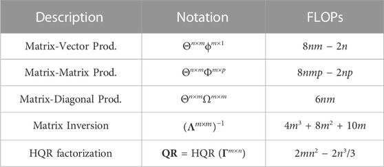
TABLE 1. Common matrix algebra computational complexity.

Moreover, Table 2 presents some useful finite sum identities (Rosen, 2010), which were widespread applied on the complexity formulation for the investigated techniques.

TABLE 2

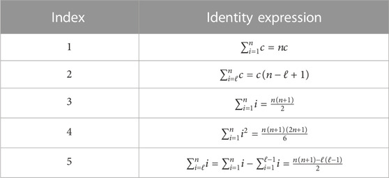
TABLE 2. Useful finite sum identities.

4 Linear estimation techniques

In this subsection, we describe the most relevant techniques on linear estimation that are commonly used in digital communications systems, such as synchronization, channel estimation, and equalization.

4.1 Linear minimum mean squared error estimator

The LMMSE is a simple implementation of the classic MMSE estimator that presents low complexity and sub-optimal performance once it is constrained to be linear. The LMMSE estimator (Huemer et al., 2017; Albreem et al., 2021a) for a random vector $\widehat{\mathbf{x}}$ is

${\widehat{\mathbf{x}}}_{\text{l}}={\mathbf{A}}_{\text{l}}\mathbf{y}+{\mathbf{b}}_{\text{l}},(11)$

where A_l and b_l are, respectively, a coefficient matrix and an offset vector that minimizes the MSE for the linear estimation of x. Sub-index l is used as an identification for the LMMSE estimator. The MSE matrix stores the covariance among the desired random vector and its estimation as

${\mathbf{E}}_{\text{l}}=\mathsf{E}\{\left(\mathbf{x}-{\widehat{\mathbf{x}}}_{\text{l}}\right){\left(\mathbf{x}-{\widehat{\mathbf{x}}}_{\text{l}}\right)}^{\mathrm{H}}\},(12)$

where ${\mathbf{E}}_{\text{l}}\in {\mathbb{C}}^{n\times n}$.

The parameters A_l and b_l, s.t. ${\mathbf{A}}_{\text{l}}\in {\mathbb{C}}^{n\times m}$ and ${\mathbf{b}}_{\text{l}}\in {\mathbb{C}}^{n\times 1}$, can be obtained introducing (11) into the optimization problem

$\underset{{\widehat{\mathbf{x}}}_{\text{l}}}{\mathrm{argmin}}\left({\mathbf{E}}_{\text{l}}\right)={\nabla }_{{\mathbf{A}}_{\text{l}},{\mathbf{b}}_{\text{l}}}{\mathbf{E}}_{\text{l}}\left(\widehat{\mathbf{x}}\right)=0,(13)$

which is detailed in Supplementary Appendix SA, yielding to

${\mathbf{A}}_{\text{l}}={\mathbf{C}}_{\mathbf{x}\mathbf{x}}{\mathbf{H}}^{\mathrm{H}}{\left(\mathbf{H}{\mathbf{C}}_{\mathbf{x}\mathbf{x}}{\mathbf{H}}^{\mathrm{H}}+{\mathbf{C}}_{\mathbf{w}\mathbf{w}}\right)}^{-1}(14)$

and

${\mathbf{b}}_{\text{l}}={\mathit{\mu }}_{\mathbf{x}}-{\mathbf{A}}_{\text{l}}\mathbf{H}{\mathit{\mu }}_{\mathbf{x}}.(15)$

Notice that for a zero mean parameter μ_x, (15) reduces to a null vector. Introducing (14) and (15) in (11) results in

${\widehat{\mathbf{x}}}_{\text{l}}={\mathbf{C}}_{\mathbf{x}\mathbf{x}}{\mathbf{H}}^{\mathrm{H}}{\left(\mathbf{H}{\mathbf{C}}_{\mathbf{x}\mathbf{x}}{\mathbf{H}}^{\mathrm{H}}+{\mathbf{C}}_{\mathbf{w}\mathbf{w}}\right)}^{-1}\left(\mathbf{y}-\mathbf{H}{\mathit{\mu }}_{\mathbf{x}}\right)+{\mathit{\mu }}_{\mathbf{x}}.(16)$

Applying the expectation operator on (16), allows us to verify that the LMMSE estimator is globally unbiased, as $\mathsf{E}\{{\widehat{\mathbf{x}}}_{\text{l}}\}=\mathsf{E}\{\mathbf{x}\}$, where the attribute global indicates that the unbiasedness condition is made on the whole parameter vector x.

The associated computational complexity of (16), in terms of FLOPs, is

${\mathcal{O}}_{\text{l}}=4m^3+16m^{2}n+8m^2+20mn+10m.(17)$

It is worth to mention that, for the specific case when n = m and H is diagonal, the operations in (16) involves only diagonal matrices, reducing the overall complexity to O_l (47n).

The error covariance matrix of the LMMSE estimator is given by

${\mathbf{E}}_{\text{l}}={\mathbf{C}}_{\mathbf{x}\mathbf{x}}-{\mathbf{C}}_{\mathbf{x}\mathbf{x}}{\mathbf{H}}^{\mathrm{H}}{\left(\mathbf{H}{\mathbf{C}}_{\mathbf{x}\mathbf{x}}{\mathbf{H}}^{\mathrm{H}}+{\mathbf{C}}_{\mathbf{w}\mathbf{w}}\right)}^{-1}\mathbf{H}{\mathbf{C}}_{\mathbf{x}\mathbf{x}},(18)$

whose diagonal represents the estimation error variance on $\widehat{\mathbf{x}}$.

4.2 Steepest-descent estimator

The steepest-descent (STPD) is an iterative procedure that can be applied to LMMSE and other estimators non-subject only to MMSE performance criteria. In particular, applying the STPD procedure to the LMMSE allows to reduce its overall complexity, once no matrix inversion is necessary. As a result, the STPD scheme can achieve the same MSE performance as the LMMSE. Consider the STPD linear estimator for (8) as

${\widehat{\mathbf{x}}}_{\text{s}}={\mathbf{A}}_{\text{s}}\mathbf{y}+{\mathbf{b}}_{\text{s}},(19)$

where A_s and b_s are, respectively, the final coefficient matrix and an offset vector that recursively converges to the MMSE criteria for the linear estimation of x. The sub-index s denotes the STPD linear estimator. The parameter ${\mathbf{A}}_{\text{s}}\in {\mathbb{C}}^{n\times m}$ can be approximated in a interactive fashion by

$\begin{array}{ll}\hfill {\mathbf{A}}_{{\text{s}}_t}& ={\mathbf{A}}_{{\text{s}}_{t-1}}+\delta \left[{\mathbf{C}}_{\mathbf{x}\mathbf{x}}{\mathbf{H}}^{\mathrm{H}}\right.\hfill \\ \hfill & \left.-{\mathbf{A}}_{{\text{s}}_{t-1}}\left(\mathbf{H}{\mathbf{C}}_{\mathbf{x}\mathbf{x}}{\mathbf{H}}^{\mathrm{H}}+{\mathbf{C}}_{\mathbf{w}\mathbf{w}}\right)\right]\hfill \end{array}(20)$

where t is an iteration index and δ is the step-size parameter which defines the behavior of the recursive algorithm. This is a crucial parameter and should be chosen carefully to guarantee a reasonable trade-off between convergence speed and stability (Sayed, 2003). The parameter ${\mathbf{b}}_{\text{s}}\in {\mathbb{C}}^{n\times 1}$ is given by

${\mathbf{b}}_{{\text{s}}_t}={\mathit{\mu }}_x-{\mathbf{A}}_{{\text{s}}_t}\mathbf{H}{\mathit{\mu }}_{\mathbf{x}},(21)$

which allows to express (19) at iteration t as

${\widehat{\mathbf{x}}}_{{\text{s}}_t}={\mathbf{A}}_{{\text{s}}_t}\left({\mathbf{y}}_t-\mathbf{H}{\mathit{\mu }}_{\mathbf{x}}\right)+{\mathit{\mu }}_{\mathbf{x}},(22)$

and finally, the instantaneous MSE ${\mathbf{E}}_{{\text{s}}_t}$ is given by

$\begin{array}{ll}\hfill {\mathbf{E}}_{{\text{s}}_t}& ={\mathbf{C}}_{\mathbf{x}\mathbf{x}}-{\mathbf{C}}_{\mathbf{x}\mathbf{x}}{\mathbf{H}}^{\mathrm{H}}{\mathbf{A}}_{{\text{s}}_t}^{\mathrm{H}}-{\mathbf{A}}_{{\text{s}}_t}\mathbf{H}{\mathbf{C}}_{\mathbf{x}\mathbf{x}}\hfill \\ \hfill & +{\mathbf{A}}_{{\text{s}}_t}\mathbf{H}{\mathbf{C}}_{\mathbf{x}\mathbf{x}}{\mathbf{H}}^{\mathrm{H}}{\mathbf{A}}_{{\text{s}}_t}^{\mathrm{H}}+{\mathbf{A}}_{{\text{s}}_t}{\mathbf{C}}_{\mathbf{w}\mathbf{w}}{\mathbf{A}}_{{\text{s}}_t}^{\mathrm{H}}.\hfill \end{array}(23)$

As ${\mathbf{A}}_{{\text{s}}_t}$ converges to the optimal solution given by (14), (23) approaches the final MSE E_s, which is equivalent to (18). Supplementary Appendix SB describes the procedure to obtain these results. It is worth to notice that the complexity to compute (19) is reduced once (20) requires no matrix inversion, although a certain amount of iterations must be considered in order to achieve convergence. Furthermore, as in the LMMSE, the prior knowledge of the signal statistic information is necessary to compute (20) and (21).

The complexity of computing (22), in terms of FLOPs, is

${\mathcal{O}}_{\text{s}}=16m^{2}n+20mn.(24)$

Notice that O_s refers to the computational effort per iteration. For the diagonal case, when n = m and H is diagonal, the complexity per iteration reduces to O_s(42n). In the next subsection, a popular algorithm based on STPD is presented as an option to further reduce the complexity and does not require previous knowledge on the exact signal statistics.

4.3 Least mean squares estimator

The least mean squares (LMS) is a widely employed adaptive algorithm solution involving unconstrained optimization problems in linear estimation. It is based on stochastic-gradient method that is obtained from steepest-descent implementation with a suitable approximation (Sayed, 2003). This approach dismiss the need to know the exact signal statistics and also performs its role through an iterative learning and tracking mechanism.

Retrieving from (9), (10) and (20), the LMS recursion can be rewritten, replacing those statistic parameters by its instantaneous approximations, leading to

${\mathbf{A}}_{{\text{lms}}_t}={\mathbf{A}}_{{\text{lms}}_{t-1}}+\delta \left[{\tilde{\mathbf{C}}}_{x_t{y}_t}-{\mathbf{A}}_{{\text{s}}_{t-1}}{\tilde{\mathbf{C}}}_{y_t{y}_t}\right],(25)$

where

${\tilde{\mathbf{C}}}_{{\mathbf{x}}_t{\mathbf{y}}_t}={\mathbf{x}}_t{\mathbf{y}}_t^{\mathrm{H}}(26)$

and

${\tilde{\mathbf{C}}}_{{\mathbf{y}}_t{\mathbf{y}}_t}={\mathbf{y}}_t{\mathbf{y}}_t^{\mathrm{H}}.(27)$

Typically, the mean of the observable RVs are not known a priori and, in order to calculate b_lms, it is necessary to employ some estimation method, as the local-mean estimator (LME) (Lin and Unbehauen, 1991), then estimate the mean information. It is also worth to highlight that, although it is not necessary to know exact values of C_xy, C_yy, μ_x and μ_y, it is mandatory to grant access to x_t and y_t while processing the recursion. In practical applications, such as channel estimation and equalization, this requirement can be addressed employing a training sequence, also known as pilot symbol, whenever the estimation procedure demands an update (Sayed, 2003; Guimarães, 2010). Thus, the LMS parameters can be defined as

${\mathbf{A}}_{{\text{lms}}_t}={\mathbf{A}}_{{\text{lms}}_{t-1}}+\delta \left({\mathbf{x}}_t{\mathbf{y}}_t^{\mathrm{H}}-{\mathbf{A}}_{{\text{lms}}_{t-1}}{\mathbf{y}}_t{\mathbf{y}}_t^{\mathrm{H}}\right)(28)$

and

${\mathbf{b}}_{{\text{lms}}_t}={\tilde{\mathit{\mu }}}_{{\mathbf{x}}_t}-{\mathbf{A}}_{{\text{lms}}_t}{\tilde{\mathit{\mu }}}_{{\mathbf{y}}_t},(29)$

where ${\tilde{\mathit{\mu }}}_{\mathbf{y}}$ is locally estimated using a recursive moving average structure as the leaky integrator (Prandoni and Vetterli, 2008) while ${\tilde{\mathit{\mu }}}_{\mathbf{x}}$ can also be estimated in the same way or, in case of employing a known sequence, it can be previously defined. Considering the local-mean estimation approach, these parameters can be obtained through the following recursions.

${\tilde{\mathit{\mu }}}_{{\mathbf{y}}_t}=\zeta {\tilde{\mathit{\mu }}}_{{\mathbf{y}}_{t-1}}+\left(1-\zeta \right){\mathbf{y}}_t(30)$

${\tilde{\mathit{\mu }}}_{{\mathbf{x}}_t}=\zeta {\tilde{\mathit{\mu }}}_{{\mathbf{x}}_{t-1}}+\left(1-\zeta \right){\mathbf{x}}_t(31)$

where ζ = (M_w − 1)/M_w is the real valued parameter that depends on the moving average window of length M_w. Finally, the LMS estimator is given by

${\widehat{\mathbf{x}}}_{{\text{lms}}_t}={\mathbf{A}}_{{\text{lms}}_t}\left({\mathbf{y}}_t-{\tilde{\mathit{\mu }}}_{y_t}\right)+{\tilde{\mathit{\mu }}}_{{\mathbf{x}}_t}.(32)$

The instantaneous estimation error is obtained directly from x_t and ${\widehat{\mathbf{x}}}_{{\text{lms}}_t}$ samples, which can be evaluated as

${\tilde{\mathbf{E}}}_{{\text{lms}}_t}=\left({\mathbf{x}}_t-{\widehat{\mathbf{x}}}_{{\text{lms}}_t}\right){\left({\mathbf{x}}_t-{\widehat{\mathbf{x}}}_{{\text{lms}}_t}\right)}^{\mathrm{H}},(33)$

and, as the algorithm converges, its magnitude decays.

Analyzing (28), while approaching the convergence state, the update term also decays and, under some conditions, i.e., the choice of a stable-convergent update coefficient, the final coefficient matrix is approximately given by

${\mathbf{A}}_{\text{lms}}={\mathbf{x}}_t{\mathbf{y}}_t^{\mathrm{H}}{\left({\mathbf{y}}_t{\mathbf{y}}_t^{\mathrm{H}}\right)}^{-1}.(34)$

By replacing (34) into (32) and taking the expectation of (33), we can obtain the expected MSE matrix of the LMS algorithm as

${\mathbf{E}}_{\text{lms}}={\mathbf{C}}_{\mathbf{x}\mathbf{x}}-{\mathbf{C}}_{\mathbf{x}\mathbf{x}}{\mathbf{H}}^{\mathrm{H}}{\left(\mathbf{H}{\mathbf{C}}_{\mathbf{x}\mathbf{x}}{\mathbf{H}}^{\mathrm{H}}+{\mathbf{C}}_{\mathbf{w}\mathbf{w}}\right)}^{-1}\mathbf{H}{\mathbf{C}}_{\mathbf{x}\mathbf{x}}.(35)$

Eq. 35 is equivalent to the LMMSE MSE matrix from (18), which is, in practical applications, a lower bound for the LMS MSE performance.

The complexity to compute (32) for each LMS iteration is

${\mathcal{O}}_{\text{lms}}=8m^{2}n+6m^2+18mn+8m+6n,(36)$

which already includes the estimator update task, incorporating the computational cost from (28) and (29). As these equations depend only on the instantaneous observations of the vectors x_t and y_t, even when the transformation matrix H is diagonal, this condition does not reduces the complexity, once the instantaneous approximations ${\tilde{\mathbf{C}}}_{{\mathbf{x}}_t{\mathbf{y}}_t}$ and ${\tilde{\mathbf{C}}}_{{\mathbf{y}}_t{\mathbf{y}}_t}$ are evaluated through the outer products in (26) and (27).

4.4 Component-wise conditionally unbiased LMMSE estimator

The CWCU-LMMSE is a constrained linear and conditionally unbiased version of MMSE estimator, where the conditional expectation of each estimated component ${\widehat{\mathbf{x}}}_{{\text{c}}_i}$ is individually forced to be equivalent to its associated indirect observable RV ${\mathbf{x}}_{c_i}$ (Huemer et al., 2017). The CWCU-LMMSE performs unbiased estimation although it can not outperform the LMMSE estimator in a MSE criteria, since it seeks to minimize the MSE under additional constraints. We assume the already defined vectors x and y as proper and jointly complex Gaussian random variables, where proper means that the real and imaginary parts are uncorrelated with equal variances. The sub-index c is used to designate the CWCU-LMMSE estimator, which can be defined as

${\widehat{\mathbf{x}}}_{\text{c}}={\mathbf{A}}_{\text{c}}\mathbf{y}+{\mathbf{b}}_{\text{c}},(37)$

where A_c and b_c are, respectively, the coefficient matrix and the offset vector that minimizes the MSE with the additional constraint $\mathsf{E}\{{\widehat{\mathbf{x}}}_{{\text{c}}_i}\mid {\mathbf{x}}_{{\text{c}}_i}\}={\mathbf{x}}_{{\text{c}}_i}$. The solution for this unbiased linear estimator, for complex proper Gaussian x_c, with mutually independent elements, is described in detail at Supplementary Appendix SC and it is given by

${\mathbf{A}}_{\text{c}}=\mathbf{D}{\mathbf{A}}_{\text{l}},(38)$

and

${\mathbf{b}}_{\text{c}}={\mathit{\mu }}_{\mathbf{x}}-{\mathbf{A}}_{\text{c}}\mathbf{H}{\mathit{\mu }}_{\mathbf{x}},(39)$

where A_l is the coefficient matrix of the LMMSE estimator and

${\mathbf{D}}_{i,i}=\frac{{\sigma }_{{\mathbf{x}}_{{\text{c}}_i}}^2}{{\mathbf{C}}_{{\mathbf{x}}_i\mathbf{x}}{\mathbf{H}}^{\mathrm{H}}{\left(\mathbf{H}{\mathbf{C}}_{\mathbf{x}\mathbf{x}}{\mathbf{H}}^{\mathrm{H}}+{\mathbf{C}}_{\mathbf{w}\mathbf{w}}\right)}^{-1}\mathbf{H}{\mathbf{C}}_{{\mathbf{x}\mathbf{x}}_i}}(40)$

are the real valued elements of the weighting diagonal matrix $\mathbf{D}\in {\mathbb{R}}^{n\times n}$, which, for x with mutually independent elements, can also be expressed as

$\mathbf{D}={\mathbf{C}}_{\mathbf{x}\mathbf{x}}\left[{\mathbf{C}}_{\mathbf{x}\mathbf{x}}{\mathbf{H}}^{\mathrm{H}}{\left(\mathbf{H}{\mathbf{C}}_{\mathbf{x}\mathbf{x}}{\mathbf{H}}^{\mathrm{H}}+{\mathbf{C}}_{\mathbf{w}\mathbf{w}}\right)}^{-1}\right.{\left.\mathbf{H}{\mathbf{C}}_{\mathbf{x}\mathbf{x}}\right]}^{-1}.(41)$

The diagonal matrix D can also be obtained performing $\mathbf{D}={\mathbf{C}}_{\mathbf{x}\mathbf{x}}\text{diag}{\left(\text{diag}\left({\mathbf{A}}_{\text{l}}\mathbf{H}{\mathbf{C}}_{\mathbf{x}\mathbf{x}}\right)\right)}^{-1}$. Considering the reduced complexity on computing the diagonal matrix inversion and also that A_l and the resultant matrix multiplication HC_xx are already available, the required computational effort on obtaining D is

${\mathcal{O}}_D=8n^{2}m+4n^2+17n.(42)$

Applying (38), (39) and (41) in (37) allows us to represent the CWCU-LMMSE estimator as

${\widehat{\mathbf{x}}}_{\text{c}}=\mathbf{D}{\mathbf{A}}_{\text{l}}\left(\mathbf{y}-\mathbf{H}{\mathit{\mu }}_{\mathbf{x}}\right)+{\mathit{\mu }}_{\mathbf{x}},(43)$

whose computational complexity in terms of FLOPs can be obtained from (17), taking into account the weighting diagonal matrix D, yielding to

$\begin{array}{ll}\hfill {\mathcal{O}}_{\text{c}}& =4m^3+16m^{2}n+8n^{2}m+8m^2\hfill \\ \hfill & +4n^2+26nm+10m+12n.\hfill \end{array}(44)$

For the case when n = m and H is diagonal, the complexity decreases to O_c(82n). The error co-variance matrix of the CWCU-LMMSE estimator is described in Supplementary Appendix SC and it is given by

${\mathbf{E}}_{\text{c}}={\left[{\mathbf{H}}^{\mathrm{H}}{\left(\mathbf{H}{\mathbf{C}}_{\mathbf{x}\mathbf{x}}{\mathbf{H}}^{\mathrm{H}}+{\mathbf{C}}_{\mathbf{w}\mathbf{w}}\right)}^{-1}\mathbf{H}\right]}^{-1}-{\mathbf{C}}_{\mathbf{x}\mathbf{x}}.(45)$

4.5 Maximum a-posteriori estimator

The maximum a-posteriori (MAP) estimator is an useful approach to incorporate prior information into the data estimation problem. The MAP estimator is based on posterior probability maximization and it is close related to MAP hypothesis testing (Yates and Goodman, 2005). Although the MAP estimator could, in some cases, result in optimum estimates, like the MSE, it can be cumbersome (or even prohibited) to determine the exactly posterior probability function. In general, the MAP estimate of the RV X given the observation Y = y is

${\widehat{\mathbf{x}}}_{\text{map}}=\underset{\mathbf{x}}{\text{argmax}}{f}_{\mathbf{X}\mid \mathbf{Y}}\left(\mathbf{x}\mid \mathbf{y}\right),(46)$

where f_X∣Y (x∣y) is the conditional distribution function of X given Y = y.

Retrieving the definition of the complex Gaussian random vectors x and y from Section 2.2, which are connected through the linear model in (8), its conditional PDF is given by the bi-variate complex Gaussian distribution (Andersen et al., 1995) as

$\begin{array}{ll}\hfill f_{\mathbf{X}\mid \mathbf{Y}}\left(\mathbf{x}\mid \mathbf{y}\right)& ={\pi }^{-1}\text{det}{\left(\mathbf{\Sigma }\right)}^{-1}\hfill \\ \hfill & \times \text{exp}\left[-{\left(\mathbf{x}-\tilde{\mathit{\mu }}\right)}^{\mathrm{H}}{\mathbf{\Sigma }}^{-1}\left(\mathbf{x}-\tilde{\mathit{\mu }}\right)\right]\hfill \end{array}(47)$

where det (⋅) is the determinant operator,

$\mathbf{\Sigma }={\mathbf{C}}_{\mathbf{x}\mathbf{x}}-{\mathbf{C}}_{\mathbf{x}\mathbf{y}}{\mathbf{C}}_{\mathbf{y}\mathbf{y}}^{-1}{\mathbf{C}}_{\mathbf{y}\mathbf{x}}(48)$

and

$\tilde{\mathit{\mu }}={\mathit{\mu }}_{\mathbf{x}}+{\mathbf{C}}_{\mathbf{x}\mathbf{y}}{\mathbf{C}}_{\mathbf{y}\mathbf{y}}^{-1}\left(\mathbf{y}-{\mathit{\mu }}_{\mathbf{y}}\right).(49)$

Analyzing (47), it is clear that its maximum probability occurs when its exponent is null, hence, when $\mathbf{x}=\tilde{\mathit{\mu }}$. This condition yields to

${\widehat{\mathbf{x}}}_{\text{map}}={\mathit{\mu }}_{\mathbf{x}}+{\mathbf{C}}_{\mathbf{x}\mathbf{y}}{\mathbf{C}}_{\mathbf{y}\mathbf{y}}^{-1}\left(\mathbf{y}-{\mathit{\mu }}_{\mathbf{y}}\right).(50)$

Finally, replacing 9) and (10) in (50) leads to

${\widehat{\mathbf{x}}}_{\text{map}}={\mathit{\mu }}_{\mathbf{x}}+{\mathbf{C}}_{\mathbf{x}\mathbf{x}}{\mathbf{H}}^{\mathrm{H}}{\left(\mathbf{H}{\mathbf{C}}_{\mathbf{x}\mathbf{x}}{\mathbf{H}}^{\mathrm{H}}+{\mathbf{C}}_{\mathbf{w}\mathbf{w}}\right)}^{-1}\left(\mathbf{y}-\mathbf{H}{\mathit{\mu }}_{\mathbf{x}}\right),(51)$

which, in this specific case, resolves to the LMMSE estimator in (16). Hence, its computational complexity is equivalent to (17),

${\mathcal{O}}_{\text{map}}=4m^3+16m^{2}n+8m^2+20mn+10m,(52)$

while the error covariance matrix corresponds to (18) and is given by

$\begin{array}{llll}\hfill {\mathbf{E}}_{\text{map}}& ={\mathbf{C}}_{\mathbf{x}\mathbf{x}}-{\mathbf{C}}_{\mathbf{x}\mathbf{x}}{\mathbf{H}}^{\mathrm{H}}{\left(\mathbf{H}{\mathbf{C}}_{\mathbf{x}\mathbf{x}}{\mathbf{H}}^{\mathrm{H}}+{\mathbf{C}}_{\mathbf{w}\mathbf{w}}\right)}^{-1}\hfill & \hfill & \mathbf{H}{\mathbf{C}}_{\mathbf{x}\mathbf{x}}.\hfill \end{array}(53)$

4.6 Bayesian Cramér-Rao bound on estimators

The BCRB defines a physical lower bound for MSE performance, which is helpful to classify whether a given estimator attains the BCRB criteria.

Since all our information is embodied in the observed data and, eventually, in our prior knowledge about the unknown parameter, the estimation accuracy depends directly on its PDFs (Kay, 1993).

The BCRB is defined as a lower bound for the MSE matrix and it is related to the inverse of the Bayesian Fisher information matrix (BFIM) I_B (Trees and Bell, 2007), which means that

${\mathbf{E}}_{\text{BCRB}}\ge {\mathbf{I}}_{\text{B}}^{-1},(54)$

where the matrix inequality means that ${\mathbf{E}}_{\text{BCRB}}-{\mathbf{I}}_{\text{B}}^{-1}$ is a non-negative definite matrix. The elements of I_B, whose row and column indexes are given by the subscripts p and q, respectively, are obtained by

$\begin{array}{ll}\hfill {\left[{\mathbf{I}}_{\text{B}}\right]}_{p,q}& =-\mathsf{E}\left\{\frac{{\partial }^2\ln f_{\mathbf{Y}\mid \mathbf{X}}\left(\mathbf{y}\mid \mathbf{x}\right)}{\partial {\mathbf{x}}_p\partial {\mathbf{x}}_q}\right\}\hfill \\ \hfill & -\mathsf{E}\left\{\frac{{\partial }^2\ln f_{\mathbf{x}}\left(\mathbf{x}\right)}{\partial {\mathbf{x}}_p\partial {\mathbf{x}}_q}\right\}.\hfill \end{array}(55)$

From the linear model in (8), replacing the corresponding PDFs

$\begin{array}{ll}\hfill f_{\mathbf{Y}\mid \mathbf{X}}\left(\mathbf{y}\mid \mathbf{x}\right)& ={\pi }^{-1}\text{det}{\left({\mathbf{C}}_{\mathbf{w}\mathbf{w}}\right)}^{-1}\hfill \\ \hfill & \times \text{exp}\left[-{\left(\mathbf{y}-\mathbf{H}\mathbf{x}\right)}^{\mathrm{H}}{\mathbf{C}}_{\mathbf{w}\mathbf{w}}^{-1}\left(\mathbf{y}-\mathbf{H}\mathbf{x}\right)\right]\hfill \end{array}(56)$

and

$\begin{array}{ll}\hfill f_{\mathbf{x}}\left(\mathbf{x}\right)& ={\pi }^{-1}\text{det}{\left({\mathbf{C}}_{\mathbf{x}\mathbf{x}}\right)}^{-1}\hfill \\ \hfill & \times \text{exp}\left[-{\left(\mathbf{x}-{\mathit{\mu }}_{\mathbf{x}}\right)}^{\mathrm{H}}{\mathbf{C}}_{\mathbf{x}\mathbf{x}}^{-1}\left(\mathbf{x}-{\mathit{\mu }}_{\mathbf{x}}\right)\right]\hfill \end{array}(57)$

in (55), allows to define the BCRB as

${\mathbf{E}}_{\text{BCRB}}={\left({\mathbf{C}}_{\mathbf{x}\mathbf{x}}^{-1}+{\mathbf{H}}^{\mathrm{H}}{\mathbf{C}}_{\mathbf{w}\mathbf{w}}^{-1}\mathbf{H}\right)}^{-1}.(58)$

5 Detection techniques

In this section we present the MLD as a reference for the performance and complexity analysis once, considering the use of multiple antennas on transmitting and receiving simultaneous streams, is able to achieve optimal performance, minimizing the BER although showing an unfeasible complexity depending on system parameters. As a countermeasure for the prohibitive computational cost, we also review two known detection techniques, one sub-optimal and one close optimal, both with affordable complexity.

5.1 Maximum likelihood detector

As presented in Section 2, the detection task at the receiver is basically a decision process applied on the received signal in order to recover the transmitted message.

Retrieving the system model presented in (8), with m ≥ n, we admit now that x holds a sequence of discrete symbols from an alphabet $\mathcal{D}\in {\mathbb{C}}^{M\times 1}$, with M distinct members. Under the common assumption that all code words from $\mathcal{D}$ are equiprobable and, in the case where w is AWGN, the maximum likelihood (ML) detector criterion yields to the minimization of the Euclidean distance (ED) (Bai and Choi, 2014), given by

${\widehat{\mathbf{x}}}_{\text{ML}}=\underset{{\tilde{\mathbf{x}}}_k\in {\mathcal{D}}^n,k=1,\dots ,M^n}{\mathrm{argmin}}\Vert \mathbf{y}-\mathbf{H}{\tilde{\mathbf{x}}}_k{\Vert }^2,(59)$

where ${\tilde{\mathbf{x}}}_k\in {\mathbb{C}}^{n\times 1}$ is the kth column vector from the set ${\mathcal{D}}^n\in {\mathbb{C}}^{n\times M^n}$, which contains all possible cross combinations of the elements in $\mathcal{D}$, taken n at a time. In general, finding the optimal solution requires an exhaustive search over all Mⁿ hypothesis (Albreem et al., 2020), yielding to a n-exponential complexity order problem. Each hypothesis contains n symbols and the MLD can be seen as a lattice structure consisting of nMⁿ nodes. The Algorithm 1 summarizes the MLD procedure whose complexity is mainly dictated by the squared ED computation of each hypothesis at line 3 and the comparison at line 5.

Algorithm 1. ML Detector.

Result: ${\widehat{\mathbf{x}}}_{\text{ML}}$

1: ρ² = ∞

2: for k ← 1 to Mⁿ do

3: $d_k^2={\sum }_{i=1}^m|y_i-{\bar{\mathbf{H}}}_i{\tilde{\mathbf{x}}}_k{|}^2$

4: if $d_k^2<{\rho }^2$ then

5: ${\rho }^2=d_k^2$

6: ${\widehat{\mathbf{x}}}_{\text{ML}}={\tilde{\mathbf{x}}}_k$

7: end if

8: end for

In the Algorithm 1, ${\bar{\mathbf{H}}}_i$ is the ith row of the matrix H and $d_k^2$ is the squared ED of the kth hypothesis. The required computational effort on MLD, in terms of FLOPs, is

${\mathcal{O}}_{\text{ML}}=M^n\left(8mn+3m+2\right).(60)$

Supposing an alphabet with 16 distinct elements and n = 8, the MLD needs a total of 4.29 × 10⁹ hypothesis tests in order to detect ${\widehat{\mathbf{x}}}_{\text{ml}}$. Although optimal, in certain applications the MLD requires a prohibited computational effort (Albreem et al., 2020). In following sub-sections, we present reduced complexity alternatives for the MLD at the expense of sub-optimal performance.

5.2 MMSE with ordering successive interference cancellation detector

The MMSE-OSIC is a non-linear estimator that attempts to improve interference cancellation in applications such as SM-MIMO, i.e., Bell Laboratories layer space-time (BLAST) variances (Hampton, 2013).

This method basically starts organizing the rows of the received sequence y and the full-rank channel matrix H in ascending order of SNR. Afterwards, starting from the last row, which holds the symbol with higher SNR, decides by the most likely transmitted information at layer ℓ through ML detection. The estimated symbol from layer ℓ = n is then used, together with CSI, to remove its interference in the foregone layer ℓ = n − 1, prior to ML detection. This procedure is repeated until all layers ℓ = n − 1, …, 1 have been processed. Finally, original ordering is reestablished undoing the initial sort operation. The idea to organize the received sequence according to SNR is to avoid error propagation, possibility that might occur in case we start the successive interference cancellation (SIC) algorithm with an arbitrary low SNR signal (Golden et al., 1999).

The ordained received vector and CSI can be obtained performing

${\mathbf{y}}_{\text{o}}=\mathbf{P}\mathbf{y}(61)$

and

${\mathbf{H}}_{\text{o}}=\mathbf{P}\mathbf{H},(62)$

where P is a m × m binary permutation matrix, built based on SNR estimation for each y element. It has exactly one entry of 1 in each row and each column, with 0s elsewhere. For example, sorting a vector in ascending order according to a given estimated SNR sequence, e.g., (Zhang et al., 2017; Giordani et al., 2020; Tapio et al., 2021), would require a left multiplication by $\mathbf{P}=\left(\begin{array}{ccc}0& 1& 0\\ 0& 0& 1\\ 1& 0& 0\end{array}\right)$. Underneath the common assumption that the constellation alphabet $\mathcal{D}$ is zero mean with normalized energy and w is AWGN, the estimated SNR at the ith receiver antenna after equalization is

${\widehat{\mathit{\gamma }}}_i={\left({\sigma }^2\Vert {\mathbf{A}}_i{\Vert }^2\right)}^{-1},(63)$

where A_i is the ith row of a linear equalization matrix, e.g., the LMMSE equalizer from (14).

Hereafter, the SIC at layer ℓ is accomplished by interference cancellation and equalization through

$\begin{array}{ll}\hfill {\bar{\mathbf{x}}}_{\text{o}}& ={\bar{\mathbf{H}}}_{{\text{o}}_j}^{\mathrm{H}}{\left({\bar{\mathbf{H}}}_{{\text{o}}_j}{\bar{\mathbf{H}}}_{{\text{o}}_j}^{\mathrm{H}}+{\mathbf{C}}_{\mathbf{w}\mathbf{w}}\right)}^{-1}\hfill \\ \hfill & \times \left({\mathbf{y}}_{\text{o}}-\sum _{\ell +1}^n{\widehat{x}}_{{\text{osic}}_{\ell +1}}{\bar{\mathbf{H}}}_{{\text{o}}_{\ell +1}}\right),\hfill \end{array}(64)$

followed by ML detection

${\widehat{x}}_{{\text{osic}}_{\ell }}=\underset{{\tilde{x}}_k\in \mathcal{D}\text{,\hspace{0.17em}}k=1,\dots ,M}{\mathrm{argmin}}\mid {\bar{x}}_{{\text{o}}_{\ell }}-{\tilde{x}}_k{\mid }^2.(65)$

In (64), ${\bar{\mathbf{x}}}_{\text{o}}$ is the ordained received vector y_o right after interference cancellation from upper layers, followed by equalization considering ${\bar{\mathbf{H}}}_{{\text{o}}_j}$, which is the jth columns of H_o for j = [1, …, ℓ]. The interference removal occurs on lower layers only, when ℓ < n, employing already detected symbols ${\widehat{x}}_{{\text{osic}}_{\ell +1}}$ and ${\bar{\mathbf{H}}}_{{\text{o}}_{\ell +1}}$, which is the ℓ + 1 column of H_o.

In (65), the sub-indexed term ${\widehat{x}}_{{\text{osic}}_{\ell }}$ is the ML detection result for layer ℓ, where ${\tilde{x}}_k$ is the kth symbol constellation from the set $\mathcal{D}$ with dimension M × 1. It is worth to mention that ${\widehat{\mathbf{x}}}_{\text{osic}}$ is already correctly ordered. Algorithm 2 is proposed for MMSE-OSIC implementation.

Algorithm 2. MMSE-OSIC.

Result: ${\widehat{\mathbf{x}}}_{\text{osic}}$

1: y_o = Py

2: H_o = PH

3: for ℓ ← n to 1 do

4: j = [1, …, ℓ]

5: ${\bar{\mathbf{x}}}_{\text{o}}={\bar{\mathbf{H}}}_{{\text{o}}_j}^{\mathrm{H}}{({\bar{\mathbf{H}}}_{{\text{o}}_j}{\bar{\mathbf{H}}}_{{\text{o}}_j}^{\mathrm{H}}+{\mathbf{C}}_{\mathbf{w}\mathbf{w}})}^{-1}({\mathbf{y}}_{\text{o}}-{\sum }_{\ell +1}^n{\widehat{x}}_{{\text{osic}}_{\ell +1}}{\bar{\mathbf{H}}}_{{\text{o}}_{\ell +1}})$

6: ${\widehat{x}}_{{\text{osic}}_{\ell }={\mathrm{arg\; min}}_{{\tilde{x}}_k\in \mathcal{D}}}\mid {\bar{x}}_{{\text{o}}_{\ell }}-{\tilde{x}}_k{\mid }^2$

7: end for

Analysing Algorithm 2 and applying the summation identity ${\sum }_{\ell =1}^n\ell =n(n+1)/2$ for the variable matrix size computations along all n − layer iterations, the estimated complexity for the MMSE-OSIC is given by

$\begin{array}{ll}\hfill {\mathcal{O}}_{\text{osic}}& =4m^{3}n+2m^2{n}^2+8m^{2}n+4m{n}^2\hfill \\ \hfill & +2m^2+6mn+10M-n^2-n.\hfill \end{array}(66)$

5.3 Sphere detector

The SD (Fincke and Pohst, 1985) is an algorithm to address the non-deterministic polynomial-time (NP) hard integer least squares (ILS) problem and achieve optimal MLD performance with an average polynomial complexity (Hassibi and Vikalo, 2005).

The principle of SD is to reduce the exhaustive search procedure over all possible code words carried out by the MLD. This is accomplished restricting the search only on hypothesis where the distance from one possible code word are within a predefined radius of a high-dimensional sphere, where each hypothesis can be seen as a path with sequentially interconnected points in a finite tree structure. Whenever a path segment reaches a cumulative distance that exceeds the sphere radius, this segment and all subsequent points are discarded, yielding to a variable complexity reduction (Larsson, 2009).

In this way, depending only on the radius parameter ρ, a trade off between performance and complexity can be trimmed. If ρ is chosen sufficiently high and kept constant, all paths might be checked and the SD behaves like the MLD. If ρ is too small, this can result in non-eligible paths. In this situation, the procedure can be repeated with an increased radius. A practical approach is to initialize ρ = ∞ or based on a code word given by a low complexity technique (Dehghani Soltani et al., 2014), e.g., the ZF or MMSE detectors (Proakis, 2007) and update the radius whenever a better hypothesis is found during the search procedure.

We start introducing the HQR factorization (Koudougnon et al., 2011) expressed as QR = HQR(H) for the full-rank channel matrix H and admitting m ≥ n, where Q ∈ C^m×m is an orthonormal matrix s.t. Q^HQ = I_m and R ∈ C^m×n is an upper-triangular matrix. Left multiplying the received vector from (8) by Q^H yields to

$\tilde{\mathbf{y}}={\mathbf{Q}}^{\mathrm{H}}\left(\mathbf{Q}\mathbf{R}\mathbf{x}+\mathbf{w}\right)=\mathbf{R}\mathbf{x}+\tilde{\mathbf{w}}.(67)$

Since Q is orthonormal, the noise distribution of $\tilde{\mathbf{w}}$ is still AWGN and the detection problem is equivalent to (59), including ${\tilde{\mathbf{x}}}_k$ definition. Thus, the SD problem can be represented by

${\widehat{\mathbf{x}}}_{\text{SD}}=\underset{{\tilde{\mathbf{x}}}_k\in {\mathcal{D}}^n,k=1,\dots ,M^n}{\mathrm{argmin}}\Vert \tilde{\mathbf{y}}-\mathbf{R}{\tilde{\mathbf{x}}}_k{\Vert }^2,(68)$

which can be addressed through a point-sequence search algorithm (Agrell et al., 2002). This structure resembles a spanning tree, with a root node located at the top layer ℓ = n, spanning to M nodes in the immediately next layer ℓ = n − 1. In this way, each node from an upper layer connects to M nodes in subsequent beneath layer. Each layer connection or path section is defined here as a segment. A series of segments connecting a root node to one of the Mⁿ nodes at the final layer ℓ = 1 forms one distinct path among Mⁿ possibilities. The total amount of nodes, η_SD, in a given spanning tree structure has a close relation with the SD complexity and can be obtained as

${\eta }_{\text{SD}}=\sum _{\ell =1}^n{M}^{\ell }.(69)$

The SD executes a top-down search along the tree while compute the squared node distance $d_{\ell }^2$ at layer ℓ under analysis given by

$d_{\ell }^2={\left|{\tilde{y}}_{\ell }-\sum _{i=\ell }^n{r}_{\ell ,i}{\tilde{x}}_i\right|}^2,(70)$

where ℓ = n, n − 1, …, 1 is the layer index and ${\tilde{x}}_i$ is one of the M distinct constellation symbols chosen from the set $\mathcal{D}$. The scalar r_ℓ,i is an element of matrix R and ${\tilde{y}}_{\ell }$ is the ℓth element of vector $\tilde{\mathbf{y}}$. When d (ℓ,s)² > ρ², subsequent layers are pruned, leading the algorithm to move on next segment direction or beginning a new path search. It is worth to mention that, in order to avoid the square root in (70), this comparison can be evaluated on the squared distances.

Algorithm 3 describes the SD mechanism to find ${\widehat{\mathbf{x}}}_{\text{sd}}$ employing a recursive function SD(ℓ) along the tree search task. For simplicity, the algorithm initializes the parameter ρ² = ∞. The variable s = 1, …, M is the segment or constellation symbol index for each node hypothesis test. It is also assumed that, when necessary, some parameters are global accessible inside the algorithm environment.

Algorithm 3. Sphere Detector.

Result: ${\widehat{\mathbf{x}}}_{\text{SD}}$

1: QR = HQR(H)

2: $\tilde{\mathbf{y}}={\mathbf{Q}}^{\mathrm{H}}\mathbf{y}$

3: ρ² = ∞

4: ℓ = n

5: function SD(ℓ)

6: for s ← 1 to M do

7: ${\tilde{x}}_{\ell }={\mathcal{D}}_s$

8: $d_{\ell }^2={\left|{\tilde{y}}_{\ell }-{\sum }_{i=\ell }^n{r}_{\ell ,i}{\tilde{x}}_i\right|}^2$

9: if $({\sum }_{i=\ell }^n{d}_i^2<{\rho }^2)$ then

10: if (ℓ == 1) then

11: ${\widehat{\mathbf{x}}}_{\text{SD}}=[{\tilde{\mathbf{x}}}_n,{\tilde{\mathbf{x}}}_{n-1},\dots ,{\tilde{\mathbf{x}}}_1]$

12: ${\rho }^2={\sum }_{i=1}^n{d}_i^2$

13: else

14: SD (ℓ − 1)

15: end if

16: end if

17: end for

18: end function

The task of finding an exact expression for the complexity of the SD is not trivial once it depends not only on the transmission channel matrix dimension but also on the sphere radius, which is, in turn, a function of the SNR. Indeed, the SD FLOPs account is a random variable with expected polynomial complexity although, in the worst case scenario, it can reach exponential complexity (Hassibi and Vikalo, 2005). Considering the worst case, where all nodes of every segment are visited, the resulting complexity is given by

${\mathcal{O}}_{\text{SD}}=O_{\text{HQR}}+O_{\tilde{\mathbf{y}}}+M^n\sum _{\ell =1}^n{O}_{\text{node}}\left(\ell \right),(71)$

where O_HQR is the complexity of the HQR factorization at line 1 of the Algorithm 3, given by Table 1, and the term $O_{\tilde{\mathbf{y}}}$ is the matrix-vector product in line 2 of the Algorithm 3. The last term in (71) represents the complexity of the recursive function SD(ℓ) with Mⁿ representing the total amount of segments in the spanning tree search that multiplies the summation over all layers, which represents a fully segment containing n nodes, connecting the uppermost layer down to layer one. Finally, O_node is the complexity of one node inspection at layer ℓ, given by

${\mathcal{O}}_{\text{node}}\left(\ell \right)=\sum _{i=\ell }^{N_{\text{T}}}8\left(N_{\text{T}}-i\right)+11.(72)$

With the aid of the identities given in Table 2, an upper bound for the SD algorithm complexity is obtained as

$\begin{array}{ll}\hfill {\mathcal{O}}_{\text{SD}}& =\frac{2n^2\left(3m-n\right)}{3}+2m\left(4m-1\right)\hfill \\ \hfill & +\frac{M^n\left(3n^3+13n^2+10n\right)}{2},\hfill \end{array}(73)$

where the last term on (73) is the predominant computational cost associated with the recursive SD(ℓ) function.

In a first glance, the worst case scenario for the SD algorithm exhibits higher complexity when compared with the MLD. This happens due the fact that every visited node requires the computation of the squared partial distances $d_{\ell }^2$. However, as the SD is able to reduce its complexity to a polynomial degree, thanks to its segment pruning behavior based on partial distances, in practice, the SD complexity is smaller than the MLD complexity, specially at high SNR. On the other hand, the MLD will always exhibits an exponential complexity, since all hypotheses are always evaluated.

There are also some slight variants of the SD algorithm that seeks to achieve a reduced (Arfaoui et al., 2016) or even fixed complexity (Larsson, 2009) at the cost of sub-optimal performance. In (Burg et al., 2005), some suitable approximations and simplifications are admitted, leading to implementations with affordable complexities.

5.4 Iterative MMSE-PIC detector

This method relies on two concepts, parallel interference cancellation and SISO channel decoding (Studer et al., 2011), exchanging refined information between these two domains in a iterative form. Differently from SIC, where data symbols are individually detected removing the interference caused by already decided symbols, the PIC estimates all data elements sharing the same radio resource jointly. The PIC performs a detection on the jth element x_j of x assuming that all its other elements, denoted by ${\mathbf{x}}_j$, are interfering terms. Rewriting 8) as

$\mathbf{y}={\bar{\mathbf{H}}}_j{x}_j+{\mathbf{H}}_j{\mathbf{x}}_j+\mathbf{w},(74)$

where ${\bar{\mathbf{H}}}_j$ is the jth column of H while ${\mathbf{H}}_j$ is H removing the jth column. Then, the PIC yields the signal ${\tilde{\mathbf{y}}}_j$ given by

$\begin{array}{ll}\hfill {\tilde{\mathbf{y}}}_j& =\mathbf{y}-{\mathbf{H}}_j{\mathit{\mu }}_{{\mathbf{x}}_j}\hfill \\ \hfill & ={\bar{\mathbf{H}}}_j{x}_j+\underset{{\tilde{\mathbf{w}}}_j}{\underbrace{{\mathbf{H}}_j\left({\mathbf{x}}_j-{\mathit{\mu }}_{{\mathbf{x}}_j}\right)+\mathbf{w}}},\hfill \end{array}(75)$

with ${\mathit{\mu }}_{{\mathbf{x}}_j}$ denoting μ_x removing the jth element, ${\tilde{\mathbf{w}}}_j$ models the noise-plus-interference, with variance HC_xxH^H + σ²I. Based on (75), all j = 1…n systems can be solved in parallel, employing independent linear estimation processes, whose, in general, require m × m matrix inversions for each x_j, normally yielding to cubic complexity order. In (Matthe et al., 2016), the authors demonstrate that this process is equivalent to a single linear estimation exploring a-priori knowledge on x.

Figure 2 illustrates the block diagram for the proposed iterative SISO MMSE-PIC detector. Its entry point considers, under the assumption of perfect synchronization and channel state information at the receiver (CSIR), the demodulated signal vector y, the equivalent MIMO CFR and the corresponding AWGN variance ${\sigma }_{\mathbf{w}}^2$. The expectation and variance of x are estimated with the help of a linear estimation function, in this case, we consider the CWCU-LMMSE estimator, and the available a-priori information ${\mathit{\mu }}_{\mathbf{x}}^{\text{a}}$ and ${\mathbf{C}}_{\mathbf{x}\mathbf{x}}^{\text{a}}$. Initially, when no a-priori information is available, these parameters are initialized as a null vector and an identity matrix, respectively. Next, the resulting posterior estimates, ${\mathit{\mu }}_{\mathbf{x}}^{\text{p}}$ and ${\mathbf{C}}_{\mathbf{x}\mathbf{x}}^{\text{p}}$, respectively obtained employing (43) and (45), are used by the soft demapping function ${\mathcal{M}}_{\text{soft}}^{-1}$ to obtain individual bit probability estimation for each data symbol, constrained by the constellation set $\mathcal{D}$. Assuming uncorrelated noise and dismissing the necessity of previous knowledge about the bit sequence, the approximated LLRs, for a given subcarrier, are efficient obtained with negligible impact on the overall detection performance (Studer et al., 2011; Matthé et al., 2018) by

$\begin{array}{ll}\hfill {\mathit{\lambda }}_{{\text{i}}_{j,b}}^{\text{p}}& =\frac{1}{\text{diag}{\left({\mathbf{C}}_{\mathbf{x}\mathbf{x}}^{\text{p}}\right)}_j}\left(\text{min}{\left|{\left({\mathit{\mu }}_{\mathbf{x}}^{\text{p}}\right)}_j-{\mathcal{D}}_b^{\left(0\right)}\right|}^2\right.\hfill \\ \hfill & \left.-\text{min}{\left|{\left({\mathit{\mu }}_{\mathbf{x}}^{\text{p}}\right)}_j-{\mathcal{D}}_b^{\left(1\right)}\right|}^2\right)\hfill \end{array}(76)$

where ${\mathit{\lambda }}_{\text{i}}^{\text{p}}\in {\mathbb{R}}^{\mu n\times 1}$ is the intrinsic LLR vector, j = 1…n, b = 0…μ − 1, with μ being the number of bits per symbol, ${\mathcal{D}}_b^{(0)}$ and ${\mathcal{D}}_b^{(1)}$ being the subsets of constellation symbols whose bth bit is 0 or 1, respectively. It is worth to mention that diverse LLRs sequences may be required when considering SM-MIMO systems employing frame structures that carry out integer multiples of a codeword, simultaneously transmitted by n antennas in multiple block symbols per frame. Thus, after properly gathering and organizing each codeword, soft decoding is performed in every iteration of PIC procedure. In case of random bit interleaving had been considered in the transmitter side, a de-interleaving function must be done prior to channel decoding. Afterwards, the same random bit interleaver operation is performed over extrinsic LLRs before soft mapping. The interleaving is an efficient option in order to improve the correction capacity. If the noise coming into channel decoding is highly correlated, then the convolutional decoder, commonly designed with a short constraint length, is more likely to make a decoding error than if the noise was independent. Since channel decoders are affected by burst errors, the interleaver spreads these errors out, allowing the decoders to operate with relative independent noise from bit to bit (Gallager, 2008).

FIGURE 2

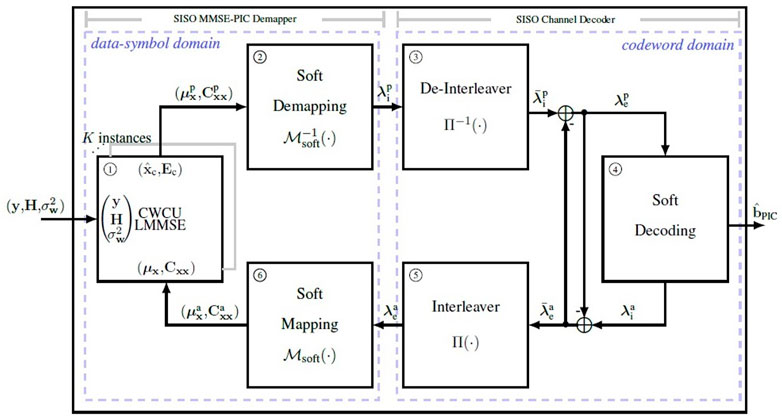
FIGURE 2. Block diagram of the Iterative MMSE-PIC detector.

The soft channel decoding is responsible for recovering the transmitted bit information from demapper estimates, obeying the code constraints. Usually, soft decoding applies algorithms able to exactly compute or approximate the APP of the information bits or, more generally, a reliability measure about each information bit. Hence, soft decoding results decoded LLRs, required in order to output re-encoded LLRs ${\mathit{\lambda }}_{\text{i}}^{\text{a}}$ for a next iteration or by taking a final hard bit decision ${\widehat{\mathbf{b}}}_{\text{PIC}}$. To improve the correctness of its decisions, both demapper and decoding have to be fed with information which does not originate from itself (Colavolpe et al., 2001), corresponding to the so called extrinsic LLRs λ_e. Without loss of generality, we assume convolutional codes as channel coding technique, which is sufficient to analyze the PIC concept. Therefore, Soft output Viterbi Algorithm (SOVA) (Hagenauer and Hoeher, 1989) is also considered hereinafter.

The extrinsic information gained during codeword domain processing, denoted by ${\mathit{\lambda }}_{\text{e}}^{\text{a}}$, is soft modulated according to (Studer et al., 2011). Let define the bth bit of the sth constellation symbol by b_s,b ∈ {0, 1} with probabilities $\mathcal{P}[{\mathbf{b}}_{s,b}=1]={[1+\exp ({\mathit{\lambda }}_{\text{e}}^{\text{a}})]}^{-1}$ and $\mathcal{P}[{\mathbf{b}}_{s,b}=0]=1-\mathcal{P}[{\mathbf{b}}_{s,b}=1]$. Then, mean and variance of the a-priory constellation symbols are updated performing

${\left({\mathit{\mu }}_{\mathbf{x}}^{\text{a}}\right)}_s=\sum _{x\in \mathcal{D}}\prod _b\mathcal{P}\left[{\mathbf{b}}_{s,b}={\mathcal{M}}^{-1}\left(x\right)\right]x(77)$

and

$\begin{array}{ll}\hfill \text{diag}{\left({\mathbf{C}}_{\mathbf{x}\mathbf{x}}^{\text{a}}\right)}_s& =\sum _{x\in \mathcal{D}}\prod _b\mathcal{P}\left[{\mathbf{b}}_{s,b}={\mathcal{M}}^{-1}\left(x\right)\right]\hfill \\ \hfill & \times \Vert x-{\left({\mathit{\mu }}_{\mathbf{x}}^{\text{a}}\right)}_s{\Vert }^2,\hfill \end{array}(78)$

This encloses the iterative MMSE-PIC loop, allowing to start a new iteration considering the a-priory information gained from soft decoding. Along successive iterations, both demapper and decoder procedures self benefit from exchanged refined information between each other. Algorithm 4 summarizes the required tasks for each iteration.

Algorithm 4. Iterative MMSE-PIC Detector.

Result: ${\widehat{\mathbf{b}}}_{\text{PIC}}$

1: for all k subcarriers do % K parallel instances, suppressed indexes

2: $({\mathit{\mu }}_{\mathbf{x}}^{\text{p}},{\mathbf{C}}_{\mathbf{x}\mathbf{x}}^{\text{p}})=\text{CWCU}-\text{LMMSE}\left[(\mathbf{y}=\mathbf{H}\mathbf{x}+\mathbf{w}),\mathcal{C}\mathcal{N}({\mathit{\mu }}_{\mathbf{x}}^{\text{a}},{\mathbf{C}}_{\mathbf{x}\mathbf{x}}^{\text{a}}),\mathcal{C}\mathcal{N}(\mathbf{0},{\sigma }_{\mathbf{w}}^2\mathbf{I})\right]$ % (43) and (45)

3: end for

4: ${\mathit{\lambda }}_{\text{i}}^{\text{p}}={\mathcal{M}}_{\text{soft}}^{-1}({\mathit{\mu }}_{\mathbf{x}}^{\text{p}},{\mathbf{C}}_{\mathbf{x}\mathbf{x}}^{\text{p}})$ % Soft Demapping according to (76)

5: ${\bar{\mathit{\lambda }}}_{\text{i}}^{\text{p}}={\mathrm{\Pi }}^{-1}({\mathit{\lambda }}_{\text{i}}^{\text{p}})$

6: ${\mathit{\lambda }}_{\text{e}}^{\text{p}}={\bar{\mathit{\lambda }}}_{\text{i}}^{\text{p}}-{\mathit{\lambda }}_{\text{e}}^{\text{a}}$

7: $({\mathit{\lambda }}_{\text{i}}^{\text{a}},{\mathbf{b}}_{\text{PIC}})=\text{SOVA}({\mathit{\lambda }}_{\text{e}}^{\text{p}})$ % Soft Decoding (Hagenauer and Hoeher, 1989)

8: ${\bar{\mathit{\lambda }}}_{\text{e}}^{\text{a}}={\mathit{\lambda }}_{\text{i}}^{\text{a}}-{\mathit{\lambda }}_{\text{e}}^{\text{p}}$

9: ${\mathit{\lambda }}_{\text{e}}^{\text{a}}=\mathrm{\Pi }({\bar{\mathit{\lambda }}}_{\text{e}}^{\text{a}})$

10: $({\mathit{\mu }}_{\mathbf{x}}^{\text{a}},{\mathbf{C}}_{\mathbf{x}\mathbf{x}}^{\text{a}})={\mathcal{M}}_{\text{soft}}({\mathit{\lambda }}_{\text{e}}^{\text{a}})$ % Soft Mapping according to (77) and (78)

With respect to computational effort comparison, it is reasonable to consider the estimation processes at line 2, detaining the majority complexity executing Algorithm 4. Since demapping and decoding are, in general, common tasks in every digital communication system, it is sufficient to express the MMSE-PIC detector complexity per iteration by

${\mathcal{O}}_{\text{PIC}}\approx K{\mathcal{O}}_{\text{c}},(79)$

The estimation stage employs up to K parallel instances of the CWCU-LMMSE estimator to solve each m × n linear systems, corresponding to the number of active subcarriers. Retrieving (44), the complexity order of Algorithm 4 is mainly dictated by a cubic behavior on the employed MIMO dimension. In order to further reduce the computational cost involved in MMSE-PIC detection, approximated estimators that avoid costly matrix inversion can be considered (Matthé et al., 2018; Zhang and Kim, 2019; Park, 2022).

5.5 Genie-aided detector

The MLD energy efficiency is commonly taken as reference for performance analysis involving alternative detectors. According to Section 5.1, the computational effort required to evaluate the ML detection is, in general, unfeasible, depending on system order, even for simulation purpose. In order to overpass this demanding condition, we can consider employing an hypothetical Genie-Aided Detector (GAD).

The GAD access additional transmission side information carried to the detector through a non-dispersive and unitary gain parallel channel, representing the genie (Eriksson et al., 1995). In the receiver side, upon decision of the transmitted data, the ED ϱ_R between the detected information $\widehat{\mathbf{x}}$ and the received signal y is compared with the ED ϱ_T of the transmitted data x and y. If ϱ_R < ϱ_T, an optimal MLD would also detect the wrong data sequence, leading to a frame error. On the contrary, when ϱ_R ≥ ϱ_T, it is assumed that the MLD would have found the correct data sequence and the detector under analysis not, accumulating a frame error. This procedure overestimates the MLD performance yielding to a lower bound on ML detection (Matthé et al., 2018). The validity of this bound is a direct consequence of the fact that any composite hypothesis test cannot perform better than the corresponding perfect measurement test (Anastasopoulos, 2003). Algorithm 5 is used to evaluate the MLD frame error rate (FER) lower bound employing a GAD.

Algorithm 5. Genie-Aided Detector.

Initialize:

1: total_frames = 0;

2: frame_error = 0;

For each iteration results: FER_ML

3: total_frames = total_frames + 1;

4: ${\varrho }_{\text{R}}^2=\Vert \mathbf{y}-\mathbf{H}\widehat{\mathbf{x}}{\Vert }^2$

5: ${\varrho }_{\text{T}}^2=\Vert \mathbf{y}-\mathbf{H}\mathbf{x}{\Vert }^2$

6: if ${\varrho }_{\text{R}}^2<{\varrho }_{\text{T}}^2$ then

7: frame_error = frame_error + 1;

8: ${\text{FER}}_{\text{ML}}=\frac{\text{frame\_error}}{\text{total\_frames}}$

9: end if

The GAD description encloses this section and finally allows to evaluate the aforementioned concepts, involving the estimation and detection techniques.

6 Simulation results

In order to demonstrate the properties of the investigated estimators and detectors, we propose three numerical examples. The first one seeks to evaluate and compare the resulting MSE on the estimation of four different RVs, each one considering a specific scenario, chosen to allow an easy visualization of its characteristic biasedness. The second example focus on the uncoded and non-iterative detection task considering a hypothetical SM-MIMO system, where a Monte Carlo simulation is conducted for the BER performance evaluation. The complexity comparison is performed, in both examples, analyzing the involved computational effort as a function of its respective cost sensitive parameters. The third example evaluates the iterative MMSE-PIC and compare its FER performance w.r.t. an overestimated and hypothetical SISO MLD with the help of a GAD.

6.1 Numerical example of linear estimation

Consider a linear system as in (8) with m = 4 and n = 4, where each element of the observable random vector y is $y_i={\sum }_{j=1}^n{H}_{i,j}{x}_j+w_i$ for i = 1, …, m.

The elements of H, x and w are mutually independent, where $w_i\sim \mathcal{C}\mathcal{N}(0,{\sigma }_{w_i}^2)$ for ${\mathit{\sigma }}_{\mathbf{w}}^2=[0.01,0.01,0.05,0.05]$, H_i,j are the elements of H and x_j is a discrete uniform RV from the set $\{e^{\text{j}(2j-1)\pi /4}+{\mu }_{x_j}\}$, with ${\mu }_{x_j}=2e^{\text{j}(2j-1)\pi /4}$ and variance ${\sigma }_{x_j}^2=1$. Here, x_j was defined in order to position each RV on different quadrants of a complex plane to facilitate its visual identification. Moreover, the linear estimation applied to a finite set of discrete RV allows to analyze the biasedness aspect of the different estimators. The co-variance of the random vectors x and w are C_xx = I_n and ${\mathbf{C}}_{\mathbf{w}\mathbf{w}}=\text{diag}({\mathit{\sigma }}_{\mathbf{w}}^2)$, respectively.

The proposed transformation matrix H = diag ([1, 0.5, 1, 0.5]) was built in order to allow the investigation of the MSE in some specific cases, varying from unitary transform coefficient and lower noise energy to low scaling factor with high noise energy. Table 3 outlines the proposed cases of study.

TABLE 3

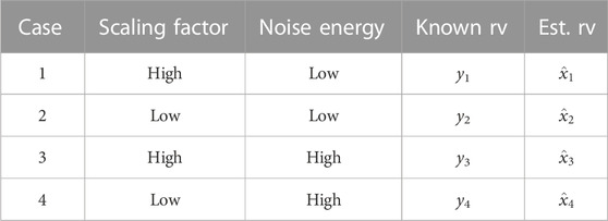
TABLE 3. Proposed cases for the performance analysis.

Figures 3–5 shown the intensity charts of the relative frequencies for each estimates in the complex plane. High incidence values are marked in red, while low occurrence values are plotted in blue. The × markers indicate possible values assumed by the discrete RVs x_j.In the top right quadrant, we have the intensity color plot for the RV x₁, corresponding to the proposed case 1 from Table 3 and, in counterclockwise direction, the remaining quadrants illustrate the resulting estimation of x₂, x₃ and x₄, respectively, related to cases 2, 3 and 4, in this order. The plot from Figure 3 reproduces the results for the LMMSE estimator and are equivalently obtained when employing STPD or MAP estimators. Figure 4 and Figure 5 show the relative frequencies obtained by the LMS estimation and the CWCU-LMMSE estimator, respectively.

FIGURE 3

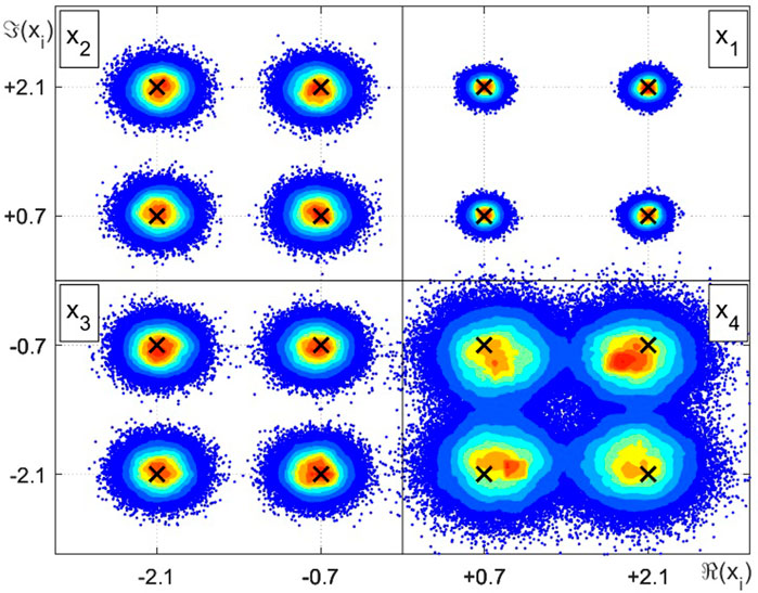
FIGURE 3. Intensity chart for the complex random variables estimation example employing LMMSE, STPD or MAP.

FIGURE 4

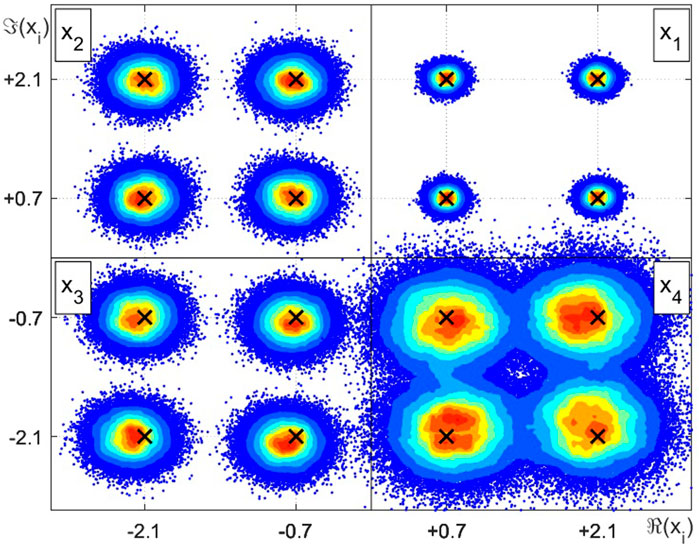
FIGURE 4. Intensity chart for the complex random variables estimation example employing LMS.

FIGURE 5

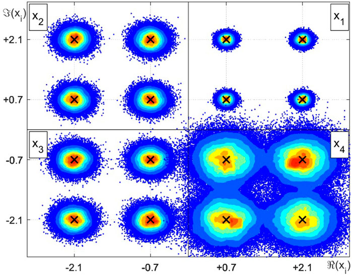
FIGURE 5. Intensity chart for the complex random variables estimation example employing CWCU LMMSE.

For the case 1, where the scaling factor equals one and the SNR is high, all estimators perform equally in terms of the MSE. This result is also observed for cases 2 (low scaling factor and high SNR) and case 3 (high scaling factor and low SNR). For case 4, with low scaling factor and low SNR, the MSE increases in relation to the other cases. In this situation, one can observe that the LMMSE, STPD and MAP estimators, whose restriction relies only on the linearity constraint, achieve the smallest MSE. The exception is the LMS estimator, which shows an poorer performance, mainly because of its built-in approximations. The CWCU-LMMSE estimator cannot outperform the LMMSE estimator in a MSE sense since it has additional constraints. However, the CWCU-LMMSE estimator features its inherent conditional unbiased property, which is evidenced in study case 4, whose result can be visualized at Figure 5. The CWCU-LMMSE has its estimates centered around the true RV events, since this estimator holds the established constraints. In contrast, the LMMSE based estimators introduce a small bias towards the prior mean, ${\mu }_{x_j}$ in order to avoid noise enhancement and attains the MMSE.

Table 4 summarizes the most relevant results for the performance analysis of the estimators considered in this review. Columns 2, 3 and 4 from Table 4 present the diagonal components of the coefficient matrix A, the elements of the offset vector b and the diagonal elements of the resulting MSE matrix E, respectively. Each element corresponds, from left to right, to the proposed cases 1 to 4, in this order. The last column shows the required computational cost in FLOPs on estimating $\widehat{\mathbf{x}}$ for each method, considering all involved operations, from the computation of A and b to $\widehat{\mathbf{x}}$ itself. It is worth to highlight that, since H is a square diagonal matrix, the overall matrix algebra complexity is reduced, except for the LMS algorithm, where, as stated in Section 4.3, it does not take advantage from a diagonal transformation matrix. Furthermore, the presented complexities for the STPD and the LMS algorithms relate to only one iteration. Although, in this specific example, the LMS algorithm exhibits to be the most costly procedure, when considering non-diagonal transformation matrices, this algorithm requires no more FLOPs than the other presented methods.

TABLE 4

TABLE 4. Linear estimation result summary.

Figure 6 illustrates the convergence behavior for the iterative STPD and LMS methods in terms of the instantaneous squared error estimation and, as expected, it decays along successive iterations. In this example, the error decreases rapidly in the first iterations, and few more are necessary to reach a stable convergence state.Figure 7 represents the amount of FLOPs as a function of the dimensions of the m × n non-diagonal transformation matrix. The STPD and the LMS iterative methods are the less costly algorithms, since no matrix inversion is involved and their complexity accounts only the amount of FLOPs per iteration. However, in practical applications, these algorithms requires no more than few iterations to converge, as exemplified by Figure 6. The LMMSE and the MAP estimators are equivalent and show intermediary complexity, while the CWCU-LMMSE is the most complex algorithm because it employs an additional weighting operation.

FIGURE 6

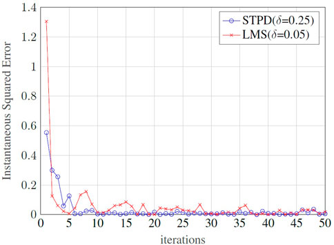
FIGURE 6. STPD and LMS convergence behavior for the proposed example.

FIGURE 7

FIGURE 7. FLOP counting for the presented linear estimators.

In Figure 8, one can visualize the MSE of the linear estimators against the BCRB. Parameter α is the noise energy and parameter β is the transformation matrix gain, where C_ww = αI_n and H = βI_n, for n = 4. The LMMSE and the MAP estimators attain the BCRB and are considered optimal in a Bayesian sense. The iterative STPD and LMS methods are, at least in theory, lower bounded by the LMMSE performance once they depend on further convergence aspects of the algorithms. As expected, the CWCU-LMMSE does not attain the BCRB and it shows low performance in terms of MSE, especially in cases with intense noise enhancement (high α and low β).

FIGURE 8

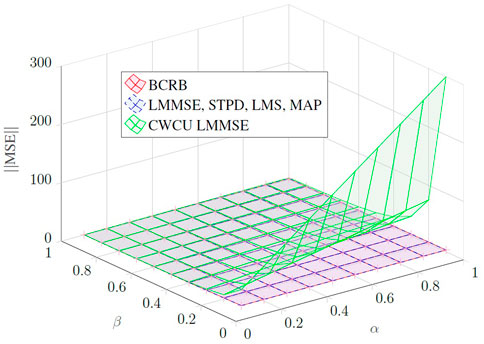
FIGURE 8. MSE versus BCRB for the investigated linear estimators.

6.2 Numerical example of non-iterative and uncoded detection in a digital communication system

In this subsection, an n × m SM-MIMO digital communication system based on the model presented in Section 2 is considered. We adopted n = m = 4 antennas for both the transmitter and receiver, such that n different data streams are transmitted simultaneously. Furthermore, no channel coding neither iterative detection are used, these are the reasons why we excluded the MMSE-PIC from this analysis. The system uses a 16-QAM to map bits into symbols, which are transmitted through a time-varying and frequency selective channel employing an orthogonal multicarrier scheme, i.e., CP protected OFDM. Assuming a symbol length with K = 64 samples, a CP with N_CP = 16 samples, which is larger than the maximum channel delay profile. In this case, the channel coherence bandwidth is wider than the bandwidth of a subcarrier and the channel frequency response can be considered to be a flat Rayleigh channel per subcarrier. We also assume perfect symbol time and carrier frequency synchronization and that the CSIR is available. The simulation parameters are given in Table 5.

TABLE 5

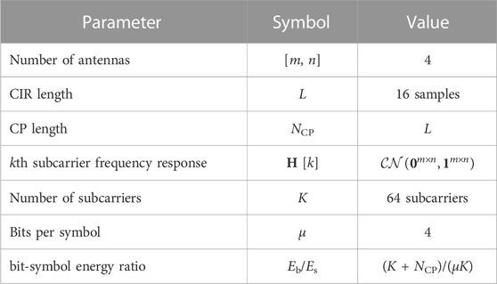
TABLE 5. Parameters for the non-iterative and uncoded system simulation.

Figure 9 illustrates some selected energy efficiency Monte Carlo simulation results. It relates the BER versus the E_b/N₀ ratio for the main presented estimation and detection techniques. The so called MMSE process performs a LMMSE equalization over the received and demodulated symbols, which can be applied in this case, since the system model is linear. The denominated CWCU-LMMSE further employs a diagonal weighting on the LMMSE equalization matrix, as demonstrated in Section 4. Then, right after equalization, ML detection is used to find the most probable transmitted sequence. According to (63), an equalization matrix is required to estimate the SNR in the MMSE-OSIC described in Algorithm 2. In this example, we used the aforementioned equalization matrices, the LMMSE and its weighted CWCU-LMMSE version. Besides these detectors, we present the results for the SD, described by Algorithm 3 The MLD, described by Algorithm 1, has also been implemented as a benchmark for the techniques considered in this paper.

FIGURE 9

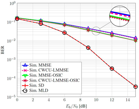
FIGURE 9. Monte Carlo simulation of an uncoded 16-QAM employing a 4 × 4 SM-MIMO-OFDM in time-varying and frequency selective channel.

The detectors exploiting the diagonal weighting, namely CWCU-LMMSE and CWCU-LMMSE-OSIC, show a slight improvement in the BER performance when compared with the corresponding MMSE and MMSE-OSIC, in this order. This small improvement is a result of a better fitting of the CWCU-LMMSE equalized signal on the constellation grid prior to detection. This characteristic holds for the Rayleigh flat-fading channel, where the symbols after CWCU LMMSE equalization remains unbiased, while the symbols equalized by the LMMSE tends to introduce a small bias towards the expected value of the discrete RV set, which, for a symmetric equiprobable QAM constellation, is zero. On the other hand, for AWGN channel, both equalizers performs equally in terms of BER (Lang and Huemer, 2015). The SD achieves a performance that is equivalent to the one observed for the MLD and over-performing all previous detectors.

In Figure 10, we analyze the SD complexity for the proposed example in terms of the average number of visited nodes at each layer. We notice that this parameters is not so dependent on the SNR as the average amount of visited nodes slight decays with the E_b/N₀. Furthermore, bottom layers are more commonly visited once the tree search structure exponentially expands towards the underneath layers. From the average number of visited nodes and (72), we obtain the average complexity in FLOPs. This is an important parameter once it allows to compare the upper bound of the SD complexity, given by (73), its average computational cost, and the MLD complexity given by (60). This behavior can be seen graphically in Figure 11, that brings the complexity growth, in log scale, of the presented detection methods, in terms of FLOPs counting as a function of the constellation size M, while assuming n = m. Among the presented detectors, the MMSE-OSIC has the lowest and restrained computational cost once that (66) follows a cubic expansion rate with the number of receive antennas. This behavior can be extended for the iterative MMSE-PIC considering the linear dependency on the number of iterations. We can also infer, as described in (73) and (60), an exponential growth in the worst case scenario for the SD and for the MLD, respectively. The average complexity of SD for the proposed example is also pointed in the graph, which confirms that, in average, the SD achieves the MLD performance at an smaller complexity (approximately 4 O_osic in this example), although it can still reach exponential computational cost.

FIGURE 10

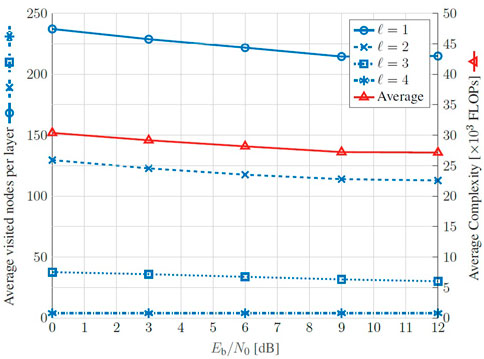
FIGURE 10. SD complexity analysis for the simulated parameters.

FIGURE 11

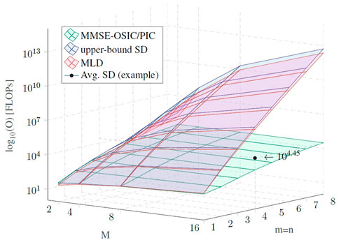
FIGURE 11. FLOP complexity comparison for the main evaluated detection methods.

It is easy to see that both SD and MLD algorithms, although optimal in terms of BER performance compared with the OSIC approach, exhibits prohibitive complexity when the modulation order or the number of antennas increases, which is the case of high order communication systems, such as massive MIMO (Albreem et al., 2019). In these cases, different solutions, in general some slight variances of the presented methods, as those already cited in Section 1, or even new proposals that might emerge from that, should also be considered.

6.3 Numerical example of iterative detection in a digital communication system

This example focus on the iterative MMSE-PIC detector, described in Section 5.4, employing a convolutional code aiming error correction capability. In order to provide an optimal reference for energy efficient comparison, we consider the GAD to emulate a SISO MLD, resulting in a hypothetical FER lower bound. We also present the results for the non-iterative detectors MMSE-OSIC and SD, both employing intra-frame interleaving, hard demapping and hard channel decoding. The simulation employs the same parameters used in the uncoded example with supplementary information given by Table 6.

TABLE 6

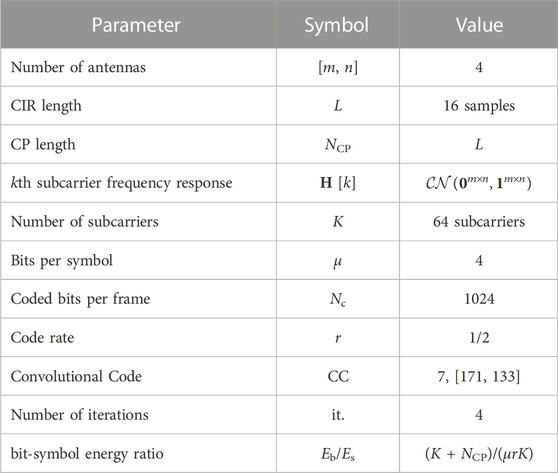
TABLE 6. Supplementary parameters for the iterative detection simulation.

Figure 12 illustrates the BER behavior for the same channel coding parameters, accenting the difference between non-iterative hard detectors and an iterative soft approach. The MMSE-OSIC poorly performs as a result of error propagation and single iteration execution. The conventional SD, although able to close achieves the ML criteria, are also still far away from the iterative MMSE-PIC once its detection is based only on the constellation constraint. It is worth to mention the availability of SISO-SD in literature (Studer and Bölcskei, 2010; Witte et al., 2010) that approaches the optimal performance in SM-MIMO applications. In this work, we replace this intricate detector by the so called genie detection.

FIGURE 12

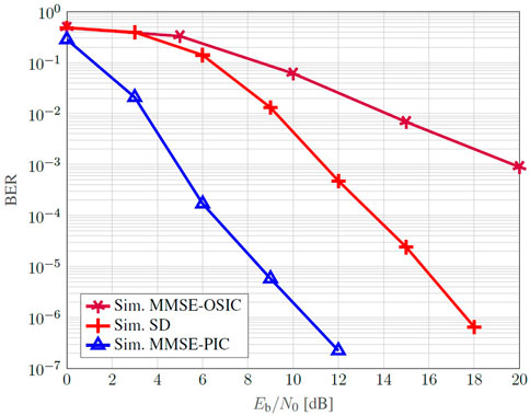
FIGURE 12. BER Monte Carlo simulation of a coded 16-QAM employing a 4 × 4 SM-MIMO-OFDM in time-varying and frequency selective channel.

In Figure 13, we analyze the FER performance w.r.t. a reference lower bound given by the GAD, based on the detected codeword from the MMSE-PIC. Whenever a bit error is detected in a codeword, the simulation accounts for a frame error. Once again, both non-iterative MMSE-OSIC and SD are positioned on the right of the iterative MMSE-PIC, this last one exhibiting a close to optimal result. This demonstrates that, among all detectors analyzed, the MMSE-PIC shows a prominent performance not only in terms of energy efficiency but also in complexity meaning, comparable to the cubic order of the MMSE-OSIC.

FIGURE 13

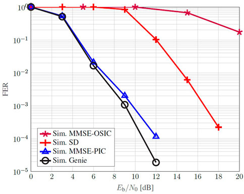
FIGURE 13. FER Monte Carlo simulation of a coded 16-QAM employing a 4 × 4 SM-MIMO-OFDM in time-varying and frequency selective channel.

7 Conclusion

In this review, linear estimators based on the classical LMMSE was discussed, including its intricate derivations, generally omitted even in textbooks. These detailed descriptions might be helpful on proposing new estimators or low complexity approximations. Regarding on complexity, a substantiated computing method is employed, based on FLOP counting for diverse involved operations, which can be a useful tool on the evaluation and comparison of different procedures. Moreover, the proposition of a BCRB permits to use an absolute reference for the MSE analysis. Although the CWCU-LMMSE MSE diverges from the BCRB in cases with potential for noise enhancement, this result does not reflect in the BER, being attributed to its unbiasedness characteristic, yielding to a better constellation grid fitting prior to detection. Note that, in similar situations, the LMMSE would also require a re-scaling in order to fit the constellation grid. In the case of the CWCU-LMMSE, this process is inherent.

With respect to detectors, those visited in this work were described through easy implementable algorithms and analysed in terms of its energy efficiency and computing cost. Although both MLD and SD achieves optimal performance, its intrinsic exponential complexity implies harsh restrictions on practical MIMO applications, s.t. small constellation sizes and few simultaneous data streams, limited by the number of transmit and receive antennas. Although the MMSE-OSIC presents affordable complexity, its performance is far from optimal. In contrast, the iterative MMSE-PIC associates expressive results, being able to closely achieves optimal performance with a computational cost comparable to the MMSE-OSIC. The iterative MMSE-PIC poses as a feasible alternative to SM-MIMO, even for massive MIMO applications, especially considering recent researches that seeks to reduce the complexity on the system solution problem, employing suitable approximations to the matrix inversion (Park, 2022).

In summary, in order to achieve the challenging and contrasting requirements of future mobile communication, different radio access techniques, among them the SM-MIMO scheme, will be a fundamental tool. In this sense, the presented tutorial contributes with a common framework that allows a fair comparison among the settled studied solutions and provides an initial guideline for researchers that are looking for a general view of the main techniques available for SM-MIMO detection and estimation.

Future works on these topics might also embrace the use of iterative estimators, specially some mixture of the STPD or the LMS with the CWCU-LMMSE weighting diagonal, in order to attain unbiasedness and avoid costly matrix inversion while keeping a channel tracking mechanism, jointly with parallel interference cancellation methods applied on non-orthogonal waveforms in SM-MIMO applications, with potential to harvest diversity while achieving multiplexing gain at the same time. Moreover, artificial intelligence is a prominent alternative to replace the statistical-based solvers discussed here by more generalist algorithms.

Author contributions

DG carried out the background research, manuscript development and simulation analysis. LM conceived the study, participated in its design, coordination and helped to write the manuscript. TP helped with the writing of the manuscript and also reviewing it. All authors read and approved the final manuscript.

Funding

This work was partially supported by the Brazil 6G project funded by RNP/MCTIC Grant No. 01245.010604/2020-14, by the SAMURAI project funded by FAPESP Grant No. 20/05127-2 and by CNPq Grand No. 303282/2021-5.

Conflict of interest

The authors declare that the research was conducted in the absence of any commercial or financial relationships that could be construed as a potential conflict of interest.

Publisher’s note

All claims expressed in this article are solely those of the authors and do not necessarily represent those of their affiliated organizations, or those of the publisher, the editors and the reviewers. Any product that may be evaluated in this article, or claim that may be made by its manufacturer, is not guaranteed or endorsed by the publisher.

Supplementary material

The Supplementary Material for this article can be found online at: https://www.frontiersin.org/articles/10.3389/frcmn.2023.968370/full#supplementary-material

References

Agrell, E., Eriksson, T., Vardy, A., and Zeger, K. (2002). Closest point search in lattices. IEEE Trans. Inf. Theory 48, 2201–2214. doi:10.1109/TIT.2002.800499

CrossRef Full Text | Google Scholar

Ahmed, I., Khammari, H., Shahid, A., Musa, A., Kim, K. S., De Poorter, E., et al. (2018). A survey on hybrid beamforming techniques in 5g: Architecture and system model perspectives. IEEE Commun. Surv. Tutorials 20, 3060–3097. doi:10.1109/COMST.2018.2843719

CrossRef Full Text | Google Scholar

Albreem, M. A., Juntti, M., and Shahabuddin, S. (2019). Massive MIMO detection techniques: A survey. IEEE Commun. Surv. Tutorials 21, 3109–3132. doi:10.1109/COMST.2019.2935810

CrossRef Full Text | Google Scholar

Albreem, M. A., Alsharif, M. H., and Kim, S. (2020). A low complexity near-optimal iterative linear detector for massive MIMO in realistic radio channels of 5G communication systems. Entropy 22, 388. doi:10.3390/e22040388

PubMed Abstract | CrossRef Full Text | Google Scholar

Albreem, M. A., Salah, W., Kumar, A., Alsharif, M. H., Rambe, A. H., Jusoh, M., et al. (2021). Low complexity linear detectors for massive MIMO: A comparative study. IEEE Access 9, 45740–45753. doi:10.1109/ACCESS.2021.3065923

CrossRef Full Text | Google Scholar

Albreem, M. A., Habbash, A. H. A., Abu-Hudrouss, A. M., and Ikki, S. S. (2021). Overview of precoding techniques for massive MIMO. IEEE Access 9, 60764–60801. doi:10.1109/ACCESS.2021.3073325

CrossRef Full Text | Google Scholar

Anastasopoulos, A. (2003). Sequence error probability lower bounds for joint detection and estimation. IEEE Trans. Commun. 51, 347–351. doi:10.1109/TCOMM.2003.809718

CrossRef Full Text | Google Scholar

Andersen, H. H., Højbjerre, M., Sørensen, D., and Eriksen, P. S. (1995). The multivariate complex normal distribution. New York, NY: Springer.

Google Scholar

Arfaoui, M. A., Ltaief, H., Rezki, Z., Alouini, M. S., and Keyes, D. (2016). Efficient sphere detector algorithm for massive MIMO using GPU hardware accelerator. Procedia Comput. Sci. 80, 21696–21808. doi:10.1016/j.procs.2016.05.377

CrossRef Full Text | Google Scholar

Bai, L., and Choi, J. (2014). Low complexity MIMO detection. New York, United States: Springer Publishing Company. Incorporated.

Google Scholar

Bensaad, A., Bensaad, Z., Soudini, B., and Beloufa, A. (2013). SISO MMSE-PIC detector in MIMO-OFDM systems. Int. J. Mod. Eng. Res. 3 (5), 2840–2847.

Google Scholar

Burg, A., Borgmann, M., Wenk, M., Zellweger, M., Fichtner, W., and Bolcskei, H. (2005). VLSI implementation of MIMO detection using the sphere decoding algorithm. IEEE J. Solid-State Circ. 40, 1566–1577. doi:10.1109/JSSC.2005.847505

CrossRef Full Text | Google Scholar

Colavolpe, G., Ferrari, G., and Raheli, R. (2001). Extrinsic information in iterative decoding: A unified view. IEEE Trans. Commun. 49, 2088–2094. doi:10.1109/26.974255

CrossRef Full Text | Google Scholar

Dahrouj, H., Alghamdi, R., Alwazani, H., Bahanshal, S., Ahmad, A. A., Faisal, A., et al. (2021). An overview of machine learning-based techniques for solving optimization problems in communications and signal processing. IEEE Access 9, 74908–74938. doi:10.1109/ACCESS.2021.3079639

CrossRef Full Text | Google Scholar

Dehghani Soltani, M., Alimadadi, M., and Amindavar, H. (2014). “A hybrid method to reduce the complexity of k-best sphere decoding algorithm,” in 2014 22nd Iranian Conference on Electrical Engineering (ICEE), 1765–1770. doi:10.1109/IranianCEE.2014.6999824

CrossRef Full Text | Google Scholar

Eriksson, H., Odling, P., Koski, T., and Borjesson, P. (1995). “A genie-aided detector with a probabilistic description of the side information,” in Proceedings of 1995 IEEE International Symposium on Information Theory, 332. doi:10.1109/ISIT.1995.550319

CrossRef Full Text | Google Scholar

Fincke, U., and Pohst, M. (1985). Improved methods for calculating vectors of short length in a lattice. Math. Comput. 44, 463–471. doi:10.2307/2007966

CrossRef Full Text | Google Scholar

Foschini, G. J. (1996). Layered space-time architecture for wireless communication in a fading environment when using multi-element antennas. Bell Labs Tech. J. 1, 41–59. doi:10.1002/bltj.2015

CrossRef Full Text | Google Scholar

Gallager, R. G. (2008). Principles of digital communication. Cambdridge, MA: Cambridge University Press. doi:10.1017/CBO9780511813498

CrossRef Full Text | Google Scholar

Giordani, M., Polese, M., Mezzavilla, M., Rangan, S., and Zorzi, M. (2020). Toward 6g networks: Use cases and technologies. IEEE Commun. Mag. 58, 55–61. doi:10.1109/MCOM.001.1900411

CrossRef Full Text | Google Scholar

Glavieux, A., and Vaton, S. (2007). Convolutional codes. Paris, France: John Wiley & Sons, 129–196. doi:10.1002/9780470612422.ch3

CrossRef Full Text | Google Scholar

Golden, G., Foschini, C., Valenzuela, R., and Wolniansky, P. (1999). Detection algorithm and initial laboratory results using V-BLAST space-time communication architecture. Electron. Lett. 35 (2), 14–16. doi:10.1049/el:19990058

CrossRef Full Text | Google Scholar

Guimarães, D. A. (2010). Digital transmission: A simulation-aided introduction with VisSim/comm. Heidelberg, Germany: Springer-Verlag Berlin Heidelberg. doi:10.1007/978-3-642-01359-1

CrossRef Full Text | Google Scholar

Gunnarsson, S., Flordelis, J., Van Der Perre, L., and Tufvesson, F. (2020). channel hardening in massive MIMO: Model parameters and experimental assessment. IEEE Open J. Commun. Soc. 1, 501–512. doi:10.1109/OJCOMS.2020.2987704

CrossRef Full Text | Google Scholar

Hagenauer, J., and Hoeher, P. (1989). “A Viterbi algorithm with soft-decision outputs and its applications,” in 1989 IEEE Global Telecommunications Conference and Exhibition ’Communications Technology for the 1990s and Beyond’, 1680–1686. doi:10.1109/GLOCOM.1989.64230

CrossRef Full Text | Google Scholar

Hampton, J. R. (2013). Introduction to MIMO communications. Cambridge, MA: Cambridge University Press. doi:10.1017/CBO9781107337527

CrossRef Full Text | Google Scholar

Hassibi, B., and Vikalo, H. (2005). On the sphere-decoding algorithm i. expected complexity. IEEE Trans. Signal Process. 53, 2806–2818. doi:10.1109/TSP.2005.850352

CrossRef Full Text | Google Scholar

Huemer, M., Lang, O., and Hofbauer, C. (2017). Component-wise conditionally unbiased widely linear MMSE estimation. Signal Process. 133, 227–239. doi:10.1016/j.sigpro.2016.10.018

CrossRef Full Text | Google Scholar

Hunger, R. (2007). Floating point operations in matrix-vector calculus. Munich, Germany: Munich University of Technology, Inst. for Circuit Theory and Signal Processing.

Google Scholar

Hussain, F., Hassan, S. A., Hussain, R., and Hossain, E. (2020). Machine learning for resource management in cellular and IoT networks: Potentials, current solutions, and open challenges. IEEE Commun. Surv. Tutorials 22, 1251–1275. doi:10.1109/COMST.2020.2964534

CrossRef Full Text | Google Scholar

Jalden, J., and Ottersten, B. (2005). On the complexity of sphere decoding in digital communications. IEEE Trans. Signal Process. 53, 1474–1484. doi:10.1109/TSP.2005.843746

CrossRef Full Text | Google Scholar

Jang, J. Y., Park, C. Y., Shin, B. S., and Song, H. K. (2021). Combined deep learning and SOR detection technique for high reliability in massive MIMO systems. IEEE Access 9, 148976–148987. doi:10.1109/ACCESS.2021.3125002

CrossRef Full Text | Google Scholar

Kaur, J., Khan, M. A., Iftikhar, M., Imran, M., and Emad Ul Haq, Q. (2021). Machine learning techniques for 5G and beyond. IEEE Access 9, 23472–23488. doi:10.1109/ACCESS.2021.3051557

CrossRef Full Text | Google Scholar

Kay, S. M. (1993). Fundamentals of statistical signal processing: Estimation theory. Hoboken, NJ: Prentice-Hall.

Google Scholar

Kobayashi, R. T., Ciriaco, F., and Abrão, T. (2014). “Performance and complexity analysis of sub-optimum MIMO detectors under correlated channel,” in 2014 International Telecommunications Symposium (ITS), 1–5. doi:10.1109/ITS.2014.6948035

CrossRef Full Text | Google Scholar

Koudougnon, H., Saadane, R., and Belkasmi, M. (2011). “Sphere decoding based on QR decomposition in STBC,” in 2011 International Conference on Multimedia Computing and Systems, 1–5. doi:10.1109/ICMCS.2011.5945624

CrossRef Full Text | Google Scholar

Lang, O., and Huemer, M. (2015). CWCU LMMSE estimation under linear model assumptions. Linz, Austria: Elsevier, 537–545. doi:10.1007/978-3-319-27340-2_67

CrossRef Full Text | Google Scholar

Larsson, E. (2009). MIMO detection methods: How they work [lecture notes]. IEEE Signal Process. Mag. 26, 91–95. doi:10.1109/MSP.2009.932126

CrossRef Full Text | Google Scholar

Lin, J., and Unbehauen, R. (1991). “A method to improve the performance of the LMS adaptive filter in processing signals of non-zero mean with sharp changes,” in 1991 IEEE International Symposium on Circuits and Systems (ISCAS), 556–559.

Google Scholar

Mahmoud, O., and El-Mahdy, A. (2021). “Performance evaluation of non-coherent dpsk signal detection algorithms in massive mimo systems,” in 2021 Telecoms Conference (ConfTELE), 1–5. doi:10.1109/ConfTELE50222.2021.9435427

CrossRef Full Text | Google Scholar

Matthe, M., Zhang, D., and Fettweis, G. (2016). “Iterative detection using MMSE-PIC demapping for MIMO-GFDM systems,”. European Wireless in 2016; 22th European Wireless Conference, 1–7.

Google Scholar

Matthé, M., Zhang, D., and Fettweis, G. (2018). Low-complexity iterative mmse-pic detection for mimo-gfdm. IEEE Trans. Commun. 66, 1467–1480. doi:10.1109/TCOMM.2017.2782339

CrossRef Full Text | Google Scholar

Mopuri, S., and Acharyya, A. (2017). Low-complexity methodology for complex square-root computation. IEEE Trans. Very Large Scale Integration (VLSI) Syst. 25, 3255–3259. doi:10.1109/TVLSI.2017.2740343

CrossRef Full Text | Google Scholar

Park, S. (2022). Low-complexity lmmse-based iterative soft interference cancellation for mimo systems. IEEE Trans. Signal Process. 70, 1890–1899. doi:10.1109/TSP.2022.3165311

CrossRef Full Text | Google Scholar

Pereira de Figueiredo, F. A. (2022). An overview of massive MIMO for 5G and 6G. IEEE Lat. Am. Trans. 20, 931–940. In portuguese. doi:10.1109/TLA.2022.9757375

CrossRef Full Text | Google Scholar

Prandoni, P., and Vetterli, M. (2008). Signal processing for communications. Communication and information sciences. Lausanne, Switzerland: EPFL Press.

Google Scholar

Proakis, J. G. (2007). Digital communications. 5th Edition. New York, United States: McGraw-Hill.

Google Scholar

Rosen, K. H. (2010). Handbook of discrete and combinatorial mathematics. Second Edition. London, United Kingdom: Chapman & Hall/CRC.

Google Scholar

Ryan, W., and Lin, S. (2009). Channel codes: Classical and modern. Cambridge, MA: Cambridge University Press. doi:10.1017/CBO9780511803253

CrossRef Full Text | Google Scholar

Sarkar, S., and Debnath, A. (2021). “Machine learning for 5G and beyond: Applications and future directions,” in 2021 Second International Conference on Electronics and Sustainable Communication Systems (ICESC), 1688–1693. doi:10.1109/ICESC51422.2021.9532728

CrossRef Full Text | Google Scholar

Sayed, A. (2003). Fundamentals of adaptive filtering. Hoboken, NJ: Wiley - IEEE.

Google Scholar

Studer, C., and Bölcskei, H. (2010). Soft–input soft–output single tree-search sphere decoding. IEEE Trans. Inf. Theory 56, 4827–4842. doi:10.1109/TIT.2010.2059730

CrossRef Full Text | Google Scholar

Studer, C., Fateh, S., and Seethaler, D. (2011). ASIC implementation of soft-input soft-output MIMO detection using MMSE parallel interference cancellation. IEEE J. Solid-State Circ. 46, 1754–1765. doi:10.1109/JSSC.2011.2144470

CrossRef Full Text | Google Scholar

Tapio, V., Hemadeh, I., Mourad, A., Shojaeifard, A., and Juntti, M. (2021). Survey on reconfigurable intelligent surfaces below 10 GHz. EURASIP J. Wirel. Commun. Netw. 2021, 175. doi:10.1186/s13638-021-02048-5

CrossRef Full Text | Google Scholar

Trees, H. L. V., and Bell, K. L. (2007). Bayesian bounds for parameter estimation and nonlinear filtering/tracking. Hoboken, NJ: Wiley-IEEE Press. doi:10.5555/1296178

CrossRef Full Text | Google Scholar

Trefethen, L. N., and Bau, D. (1997). Numerical linear algebra. Philadelphia, PA: SIAM.

Google Scholar

Witte, E. M., Borlenghi, F., Ascheid, G., Leupers, R., and Meyr, H. (2010). “A scalable vlsi architecture for soft-input soft-output single tree-search sphere decoding,” in IEEE Transactions on Circuits and Systems II: Express Briefs, 706–710. doi:10.1109/TCSII.2010.2056014

CrossRef Full Text | Google Scholar

Yates, R. D., and Goodman, D. J. (2005). Probability and stochastic processes. 2nd ed. edn. Hoboken, NJ: John Wiley & Sons.

Google Scholar

Ye, H., Li, G. Y., and Juang, B. H. (2018). Power of deep learning for channel estimation and signal detection in OFDM systems. IEEE Wirel. Commun. Lett. 7, 114–117. doi:10.1109/LWC.2017.2757490

CrossRef Full Text | Google Scholar

Zhang, M., and Kim, S. (2019). Evaluation of mmse-based iterative soft detection schemes for coded massive mimo system. IEEE Access 7, 10166–10175. doi:10.1109/ACCESS.2018.2889728

CrossRef Full Text | Google Scholar

Zhang, D., Matthé, M., Mendes, L. L., and Fettweis, G. (2017). A study on the link level performance of advanced multicarrier waveforms under MIMO wireless communication channels. IEEE Trans. Wirel. Commun. 16, 2350–2365. doi:10.1109/TWC.2017.2664820

CrossRef Full Text | Google Scholar

Glossary

1G first generation

5G fifth generation

6G sixth generation

APP A-Posteriori Probability

AWGN additive white Gaussian noise

BCRB Bayesian Cramer-Rao bound

BER bit error rate

BLAST Bell Laboratories layer space-time

BFIM Bayesian Fisher information matrix

BS base station

CC Convolutional Code

CFLOP complex float-point operation

CFR channel frequency response

CIR channel impulse response

CP cyclic prefix

CSI channel state information

CSIR channel state information at the receiver

CWCU component-wise conditionally unbiased

DFT discrete Fourier transform

ED Euclidean distance

FEC forward error correction

FER frame error rate

FLOP float-point operation

GAD Genie-Aided Detector

HQR Householder QR factorization

IAI inter-antenna interference

ILS integer least squares

iid independent and identically distributed

ISI intersymbol interference

LLR log-likelihood ratio

LME local-mean estimator

LMS least mean squares

LMMSE linear minimum mean squared error

MAP maximum a-posteriori

MIMO multiple-input multiple-output

ML maximum likelihood

MLD Maximum Likelihood Detector

MSE mean squared error

MMSE minimum mean squared error

OSIC ordering successive interference cancellation

MSE mean-squared error

NP non-deterministic polynomial-time

OFDM orthogonal frequency division multiplexing

OSIC ordering successive interference cancellation

PDF probability density function

PHY physical layer

PIC Parallel Interference Cancellation

QAM Quadrature Amplitude Modulation

QoS quality of service

RIS reconfigurable intelligent surfaces

RV random variable

SD sphere detector

SIC successive interference cancellation

SISO soft-input soft-output

SM spatial multiplexing

SM-MIMO spatial multiplexing multiple-input multiple-output

SNR signal-to-noise ratio

SOVA Soft output Viterbi Algorithm

STPD steepest-descent

UE user equipment

ZF zero-forcing