A fast temporal multiple sparse Bayesian learning-based channel estimation method for time-varying underwater acoustic OFDM systems

In this paper, a fast temporal multiple sparse Bayesian learning (FTMSBL)-based channel estimation method for underwater acoustic (UWA) orthogonal frequency division multiplexing (OFDM) systems is proposed, which is optimized using the fast marginalized likelihood maximization method. The algorithm fully uses the consistent sparse structure and time-domain correlation properties of channels to improve the reconstruction performance and computational efficiency, offering better performance and higher computational efficiency than the traditional Bayesian learning algorithms. At the same time, the FTMSBL algorithm does not require computing the inverse of large matrices and consumes very little storage resources in the operation, making it suitable for hardware implementation. Simulation and sea trial results show that the FTMSBL-based underwater channel estimation algorithm achieves higher channel estimation accuracy than the orthogonal matching tracking algorithm, and the system bit error rate (BER) is significantly reduced; specifically, the FTMSBL algorithm can achieve optimal performance in strong time-dependent channels.

1 Introduction

In the last few decades, orthogonal frequency division multiplexing (OFDM) has made significant progress in the development of underwater acoustic communication technology (Li et al., 2008; Mason et al., 2008; Qiao et al., 2020, 2019; Wang et al., 2015). However, the OFDM system is more sensitive to symbol interference and Doppler frequency offset (Ma et al., 2015; Qarabaqi and Stojanovic, 2013). Exploiting the estimated channel matrix and incorporating a preprocessing step consisting of coarse timing estimation can notably reduce the input size and improve the computational efficiency (Naoumi et al., 2024). Therefore, the acquisition of UWA channel state information is an indispensable and critical part of the communication system and represents one of the research difficulties.

Traditional channel estimation algorithms include the least squares (LS) algorithm and the minimum mean square error (MMSE) algorithm. The LS algorithm is very sensitive to environmental noise, and the accuracy of channel state information is poor. The MMSE algorithm utilizes the second-order statistics of the channel, which greatly improves the quality of channel estimation. However, this algorithm requires known channel statistics and high algorithm complexity. In recent years, the sparsity of the underwater acoustic channels has been exploited. The channel impulse response presents an obvious sparse structure, and the energy is concentrated in a few paths. Therefore, the sparse channel estimation method based on compressed sensing (CS) theory has been proposed (Berger et al., 2010; Huang et al., 2010). Berger constructed the channel observation matrix with residual Doppler frequency offset using an orthogonal matching pursuit (OMP) algorithm to jointly estimate the UWA channel impulse response and Doppler factor. As we know, the UWA channel is a typical time-varying sparse channel; thus, the temporal correlation can be used to improve the accuracy of channel estimation (Huang et al., 2013; Tan et al., 2011). Zhou et al. (2017) proposed a multipath selection SOMP algorithm based on the correlation between adjacent data block channels, which achieves relatively obvious improvement in signal-to-noise ratio and bit error rate (BER) performance. However, these methods merely focused on using path delays of the OFDM block, ignoring temporal correlation for gains, which is more common in underwater acoustic channels.

Recently, sparse Bayesian learning has been used in underwater acoustic OFDM channel estimation methods (Prasad et al., 2014; Jia et al., 2022). Qiao et al. (2018) proposed a temporal multiple SBL (TMSBL)-based channel estimator to jointly estimate the channels. This method exploits the prior distribution and space–time information of the channel, adopting time correlation between OFDM block channels to improve the performance of channel estimation. However, the TMSBL algorithm has low computational efficiency, and the complexity of matrix inversion is high. Therefore, it is necessary to obtain an algorithm with high accuracy and low complexity (Cho 2022; Feng et al., 2023; Wang et al., 2021; Guo et al., 2014).

In this paper, we propose a fast temporal multiple sparse Bayesian learning-based channel estimation method in the UWA OFDM system. The method is optimized using the fast marginalized likelihood maximization method, which can optimize the computational efficiency of TMSBL. At the same time, the proposed method adopts channel coherence between consecutive OFDM blocks to improve the performance of bit error rate. We investigate the performance of the proposed channel estimator through simulations and experimental data.

2 System model design

2.1 CP-OFDM system

A passband transmit cyclic prefix (CP)-OFDM signal in continuous time can be expressed as follows:

$\stackrel{\sim }{w}\left(t\right)=2\text{Re}\left\{{\displaystyle \sum _{k=-K/2}^{K/2-1}}{w}_k{e}^{j2\pi f_{k}t}q\left(t\right)\right\},$

where $w_k$ is the transmitted symbol; $K$ is the number of subcarriers in one OFDM block, including data subcarriers $K_d$, pilot subcarriers $K_p$, and null subcarriers $K_n$. $f_k=f_c+k/T$ is the frequency of the kth subcarriers; and $f_c$ is the carrier frequency. Let $T$ denote one OFDM symbol duration, and $T_{cp}$ denote the length of the circular prefix. $q\left(t\right)$ is the pulse-shaping filter:

$\mathrm{q}\left(\mathrm{t}\right)=\left\{\begin{array}{l}1,\mathrm{t}\in \left[-{\mathrm{T}}_{\text{cp}},\mathrm{T}\right]\\ 0,\text{otherwise}\end{array}\right..$

Figure 1 shows the system model of UWA OFDM communication. Each vertical column in a frame represents an OFDM block; each grid in one vertical column represents each subcarrier frequency; the blue grids indicate the position of the inserted pilots; the white grids indicate the position of the transmitted data. The comb-shaped pilots are integrated into each OFDM block at the same interval in the frequency domain, which can better estimate and compensate for UWA channels in OFDM communication.

Figure 1

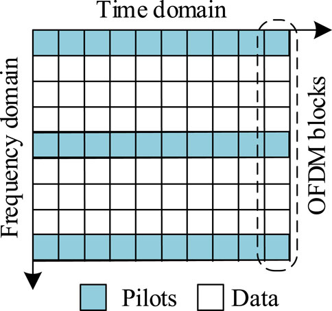
Figure 1. Structure of data and pilot subcarriers.

In OFDM communication, a frame signal contains multiple OFDM blocks. Each block needs to be estimated and demodulated individually. The cycle prefixes are in the front of the blocks to prevent symbol interference. Pilots are inserted into each block at four equal intervals. The specific frame structure is shown in Figure 2.

Figure 2

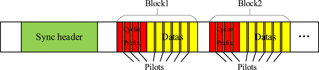
Figure 2. Structure of one-frame OFDM signal.

2.2 Receive processing

We assume that the time-varying underwater acoustic channel is a multipath channel containing $M$ paths; ${\beta }_m$ and ${\tau }_m$ are the gain and delay of the mth path, and $a$ is the Doppler factor. In addition, we assume that these parameters are constant within one CP-OFDM block duration. Then, the channel impulse response can be written as follows:

$h\left(\tau ,t\right)={\displaystyle \sum _{m=1}^M}{\beta }_m\delta \left(\tau -\left({\tau }_m-at\right)\right).$

The received passband signal is as follows:

$\stackrel{\sim }{y}\left(t\right)={\displaystyle \sum _{m=1}^M}{\beta }_m\stackrel{\sim }{w}\left(\left(1+a\right)t-{\tau }_m\right)+\stackrel{\sim }{z}\left(t\right),$

where $\stackrel{\sim }{z}\left(t\right)$ is the additive noise. The method of CP self-correlators is used to estimate Doppler block by block, and then the received signal is resampled with Doppler factor $a$. After Doppler estimation and resampling, the Doppler effect of the signal is considered to have been removed. We can model the $K\times 1$ received signal $\mathbf{Y}$ for the nth block as follows:

$\mathbf{Y}\left[n\right]=\mathbf{W}\left[n\right]\mathbf{F}\mathbf{h}\left[n\right]+\mathbf{Z}\left[n\right],$

where $\mathbf{W}\left[n\right]$ is the $K\times K$ dimensional diagonal matrix consisting of transmitted symbols. $\mathbf{Z}\left[n\right]$ is the noise vector. $\mathbf{F}$ is the $K\times M$ discrete Fourier transform (DFT) matrix. The overall channel is represented as $\mathbf{h}\left[n\right]=\left[h_1\left[n\right],h_2\left[n\right],\dots ,h_M\left[n\right]\right]$, where most of the multipath delay amplitude parameters are 0. One frame consists of $N$ consecutive OFDM blocks, so $n\in \left[1,N\right]$. The received model considering only $P$ pilot subcarriers can be written as follows:

${\mathbf{Y}}_{\mathit{p}}\left[n\right]={\mathbf{W}}_{\mathit{p}}\left[n\right]{\mathbf{F}}_{\mathit{p}}\mathbf{h}\left[n\right]+{\mathbf{Z}}_{\mathit{p}}\left[n\right],$

where ${\mathbf{Y}}_p\left[n\right]$ is the $K\times 1$ dimensional pilot reception vector, the diagonal matrix of the transmission pilot is ${\mathbf{W}}_p\left[n\right]$, and ${\mathbf{Z}}_p\left[n\right]$ is the noise vector.

3 Sparse channel estimation

3.1 Joint channel model

The underwater acoustic channel is a typical time-varying sparse channel, with a small number of sparse non-zero paths. The consecutive OFDM symbols have a stable multi-path structure of the channel, which has a temporal correlation for gains. Therefore, we model a sparse channel matrix of $N$ consecutive OFDM symbols as follows:

$\overline{\mathbf{h}}\triangleq \left[h\left[1\right],\dots ,h\left[n\right],\dots ,h\left[N\right]\right],$

where $h\left[n\right]n\in \left[1,N\right]$ represents the channel impulse response of the nth OFDM symbol. For each channel vector, the non-zero path shows joint sparsity. The $P\times M$ dimensional dictionary matrix is shown as follows:

${\mathrm{\Phi }}_{\mathit{p}}\left[n\right]={\mathbf{W}}_p\left[n\right]{\mathbf{F}}_{\mathit{p}}.$

The consecutive OFDM symbols have the same pilots. Therefore, we can model a joint estimation model for $N$ consecutive OFDM blocks as follows:

${\overline{\mathbf{Y}}}_{\mathit{p}}\left[n\right]={\mathrm{\Phi }}_{\mathit{p}}\overline{\mathbf{h}}+{\overline{\mathbf{Z}}}_{\mathit{p}},(1)$

where

${\overline{\mathbf{Y}}}_{\mathit{p}}=\left[{\mathbf{Y}}_p\left[1\right],\dots ,{\mathbf{Y}}_p\left[n\right],\dots ,{\mathbf{Y}}_p\left[N\right]\right],$

${\overline{\mathbf{W}}}_{\mathit{p}}=\left[{\mathbf{W}}_p\left[1\right],\dots ,{\mathbf{W}}_p\left[n\right],\dots ,{\mathbf{W}}_p\left[N\right]\right].$

3.2 TMSBL-based multi-block joint processing

For the estimation problem in Equation 1, we adopt the TMSBL algorithm to jointly estimate the channel matrix $\overline{\mathbf{h}}$. First, we model ${\overline{\mathbf{h}}}_i$ as the ith sparse block of $\overline{\mathbf{h}}$, and assume that all sparse signal blocks are independent. The parametric form of the prior of each ${\overline{\mathbf{h}}}_i$ is as follows:

$p\left({\overline{\mathbf{h}}}_i;{\gamma }_i,{\mathbf{B}}_i\right)\sim \mathcal{C}\mathcal{N}\left(0,{\gamma }_i{\mathbf{B}}_i\right)i=1,\dots ,M,$

where ${\gamma }_i$ is a non-negative hyperparameter that determines the sparsity of the current block and the channel length is $M$. ${\mathbf{B}}_i$ is a positive definite time correlation matrix, representing the time correlation structure of $\overline{\mathbf{h}}$. ${\gamma }_i$ and ${\mathbf{B}}_i$ are unknown hyperparameters that can be estimated in the TMSBL algorithm. We denote $\mathrm{\Gamma }$ as a $M\times M$ diagonal matrix with $\gamma$. Through the prior distribution of each sparse block, the overall prior distribution of all sparse blocks can be obtained as follows:

$p\left({\overline{\mathbf{h}}}_i;\mathrm{\Gamma },{\mathbf{B}}_i\right)={\displaystyle \prod _{i=1}^M}p\left({\overline{\mathbf{h}}}_i;{\gamma }_i,{\mathbf{B}}_i\right).$

According to the prior distribution ${\overline{\mathbf{h}}}_i$ and likelihood function $p\left({\overline{\mathbf{Y}}}_p|\overline{\mathbf{h}}\right)$, using Bayesian criterion, we can obtain the posterior probability density of $\overline{\mathbf{h}}$ as follows:

$p\left(\overline{\mathbf{h}}\left[n\right]|{\overline{\mathbf{Y}}}_{\mathit{p}};\mathrm{\Gamma }\right)=\mathcal{C}\mathcal{N}\left(\mathrm{\mu }\left[n\right],\mathrm{\Sigma }\right)n\in \left[1,N\right].$

The covariance and mean are

$\mathbf{\Sigma }={\left({\sigma }^{-2}{\mathrm{\Phi }}_P^H{\mathrm{\Phi }}_P+{\mathrm{\Gamma }}^{{\left(r\right)}^{-1}}\right)}^{-\mathbf{1}},(2)$

$\mathcal{M}=\left[\mathbf{\mu }\left[1\right],\dots ,\mathbf{\mu }\left[N\right]\right]{=\sigma }^{-2}{\mathbf{\Sigma }\mathbf{\Phi }}_P^H{\overline{\mathbf{Y}}}_p.(3)$

The $\mathrm{\mu }\left[n\right]$ is the estimated $\mathbf{h}\left[n\right]$, and the hyperparameter ${\gamma }_i$ and time correlation matrix ${\mathbf{B}}_i$ can be estimated using the EM algorithm, which obtains the parameter by iterative calculation. In the rth iteration, the E step calculates the expectation of variables under conditional probability distribution using Equations 2, 3, and the M-step is expressed via the following updated rule:

${\gamma }_i=\frac{1}{M}{\mathcal{M}}_i{\mathbf{B}}^{-\mathbf{1}}{\mathcal{M}}_i^H+{\mathrm{\Sigma }}_{ii}.$

It is worth noting that if each ${\mathbf{B}}_i$ is estimated independently, it will lead to overfitting by limited samples and too many parameters; therefore, we use one positive definite matrix $\mathbf{B}$ to model all the temporal correlation matrices ${\mathbf{B}}_i$ (Zhang and Rao, 2011; Cawley and Nicola, 2007; Guyon et al., 2010):

$\mathbf{B}={\displaystyle \sum _{i=1}^M}\frac{{\mathcal{M}}_i^H{\mathcal{M}}_i}{{\gamma }_i}+\eta {\mathbf{I}}_N.$

The noise variance can be calculated using null subcarriers as follows:

${\sigma }^2=E\left\{{\left|{\overline{\mathbf{Y}}}_{\mathit{n}}\right|}^2\right\}.$

The steps of the TMSBL algorithm are provided in Table 1.

Table 1

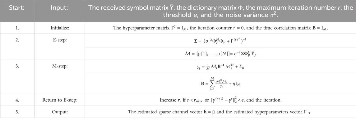
Table 1. Process of TMSBL channel estimation.

3.3 FTMSBL-based multi-block joint processing

For the estimation problem in Equation 1, we directly list the posterior probability density and likelihood function as follows:

$p\left(\overline{\mathbf{h}}\left[n\right]|{\overline{\mathbf{Y}}}_{\mathit{p}};\mathbf{\Gamma },\mathbf{B}\right)=\mathcal{C}\mathcal{N}\left(\mathrm{\mu }\left[n\right],\mathbf{\Sigma },\mathbf{B}\right)n\in \left[1,N\right],$

$p\left({\overline{\mathbf{Y}}}_{\mathit{p}}|\mathbf{\Gamma },\mathbf{B}\right)=\mathcal{C}\mathcal{N}\left(\mathbf{0},{\mathbf{C}}_{\mathit{A}},\mathbf{B}\right),$

where $\mathbf{\Gamma }={diag}^{-1}\left(\left\{{\gamma }_i\right\}\right)$ is the $M\times M$ diagonal hyperparameter matrix and the covariance and mean are ${\mathbf{\Sigma }}_{\mathrm{A}}^{-1}={\mathbf{\Gamma }}^{-1}+{\sigma }^{-2}{\mathbf{\Phi }}_{\mathrm{P}}^{\mathrm{H}}{\mathbf{\Phi }}_{\mathrm{P}}$ and $\mathbf{\mu }={\sigma }^{-2}{\mathbf{\Sigma }}_A{\mathbf{\Phi }}_P^H\mathbf{Y}$, respectively. We define the parameter ${\mathbf{C}}_{\mathrm{A}}={\sigma }^{-2}{\mathbf{I}}_{\mathrm{M}}+{\mathbf{\Phi }}_{\mathrm{P}}^{\mathrm{H}}\mathrm{\Gamma }{\mathbf{\Phi }}_{\mathrm{P}}$, where the noise variance is ${\sigma }^2$. The cost function $\mathcal{L}$ of the temporal correlation MMV model can be obtained using the type-2 maximum likelihood estimation method (Tipping, 2001):

$\mathcal{L}=Mlog\left|\mathbf{B}\right|+Nlog\left|{\mathbf{C}}_A\right|+Tr\left[{\mathbf{B}}^{-1}{\overline{\mathbf{Y}}}_P^H{\mathbf{C}}_A^{-1}{\overline{\mathbf{Y}}}_{\mathit{p}}\right],$

$=\mathcal{L}\left(\mathbf{B}\right)+\mathcal{L}\left(\left\{{\gamma }_i,{\sigma }^{-2},\mathbf{B}\right\}\right),$

where one frame consists of $N$ consecutive OFDM blocks and the channel length is $M$.

$\mathcal{L}\left(\mathbf{B}\right)\propto Mlog\left|\mathbf{B}\right|+Tr\left[{\mathbf{B}}^{-1}{\overline{\mathbf{Y}}}_P^H{{\mathbf{C}}_A^{\left(i+1\right)}}^{-1}{\overline{\mathbf{Y}}}_{\mathit{p}}\right],$

$\mathcal{L}\left(\left\{{\gamma }_i,{\sigma }^{-2},\mathbf{B}\right\}\right)\propto Nlog\left|{\mathbf{C}}_A\right|+Tr\left[{{\mathbf{B}}^{\left(i\right)}}^{-1}{\overline{\mathbf{Y}}}_P^H{{\mathbf{C}}_A^{-1}\overline{\mathbf{Y}}}_{\mathit{p}}\right].(4)$

Through the optimization of $\mathcal{L}$, we can obtain the updated formula of parameter estimation. First, we calculate the partial derivative of $\mathcal{L}\left(\mathbf{B}\right)$ to update the formula of the time domain correlation matrix $\mathbf{B}$:

$\frac{\partial \mathcal{L}\left(\mathbf{B}\right)}{\partial \mathbf{B}}=M{\mathbf{B}}^{-1}-{\mathbf{B}}^{-1}{\overline{\mathbf{Y}}}_P^H{\mathbf{C}}_A^{-1}{\mathbf{B}}^{-1}.$

We adopt the learning rule for B using $\frac{\partial \mathcal{L}\left(\mathbf{B}\right)}{\partial \mathbf{B}}=0$:

$\mathbf{B}=\frac{{\overline{\mathbf{Y}}}_P^H{\mathbf{C}}_A^{-1}{\overline{\mathbf{Y}}}_{\mathit{p}}}{M}.$

Furthermore, the noise variance ${\sigma }^2$ is obtained using the null subcarriers. We rewrite Equation 4 using the Woodbury formula to obtain the model as follows:

$\mathcal{L}\left(\left\{{\gamma }_i\right\}\right)=Nlog\left|{\mathbf{C}}_{-i}\right|+Tr\left[{\mathbf{B}}^{-1}{\overline{\mathbf{Y}}}_P^H{{\mathbf{C}}_{-i}^{-1}\overline{\mathbf{Y}}}_{\mathit{p}}\right]$

$+Nlog\left(1+{\gamma }_i{\mathbf{s}}_i\right)-Tr\left[\frac{{\mathbf{B}}^{-1}}{{\gamma }^{-1}+s_i}{\mathbf{q}}_{\mathit{i}}^{\mathit{H}}{\mathbf{q}}_{\mathit{i}}\right],$

$=\mathcal{L}\left(-i\right)+\mathcal{L}\left(i\right),$

where

$\mathcal{L}\left(-i\right)\triangleq Nlog\left|{\mathbf{C}}_{-i}\right|+Tr\left[{\mathbf{B}}^{-1}{\overline{\mathbf{Y}}}_P^H{{\mathbf{C}}_{-i}^{-1}\overline{\mathbf{Y}}}_{\mathit{p}}\right],(5)$

$\mathcal{L}\left(i\right)\triangleq \mathit{log}\left(1+{\gamma }_i{\mathbf{s}}_i\right)-Tr\left[\frac{{\mathbf{B}}^{-1}}{{\gamma }^{-1}+s_i}{\mathbf{q}}_i^H{\mathbf{q}}_i\right],(6)$

which only depends on ${\gamma }_i$. From Equations 5, 6, we can obtain the following:

${\mathbf{C}}_{-i}\triangleq {\sigma }^2\mathbf{I}+{\displaystyle \sum _{j,j\ne i}^M}{\gamma }_j{{\mathbf{\Phi }}_j\mathbf{\Phi }}_j^H,$

${\mathbf{s}}_i\triangleq {\mathbf{\Phi }}_i^H{{\mathbf{C}}_{-i}^{-1}\mathbf{\Phi }}_i,$

${\mathbf{q}}_i\triangleq {\mathbf{\Phi }}_i^H{\mathbf{C}}_{-i}^{-1}\mathbf{Y}.$

Setting $\frac{\partial \mathcal{L}\left(i\right)}{\partial {\gamma }_i}=0$, we have the following updated rule:

${\gamma }_i=\frac{{\mathbf{q}}_i{\mathbf{B}}^{-1}{\mathbf{q}}_i^H/N-{\mathbf{s}}_i}{{\mathbf{s}}_i^2}.(7)$

It should be noted that the updated result obtained from Equation 7 is a scalar, where ${\mathbf{q}}_i{\mathbf{B}}^{-1}{\mathbf{q}}_i^H$ is ${‖{\mathbf{q}}_i‖}_{\mathbf{B}}^{\mathbf{2}}$, which is the norm of the covariance matrix $\mathbf{B}$.

The steps of the FTMSBL algorithm are provided in Table 2.

Table 2

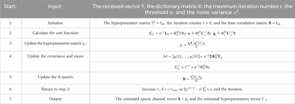
Table 2. Process of FTMSBL channel estimation.

3.4 Complexity

The computational complexity of the TMSBL algorithm mainly consists of covariance $\mathrm{\Sigma }$ and mean. The covariance can be solved with marginal cost $\mathcal{O}\left(M^3\right)$.The computational complexity of mean is $\mathcal{O}\left({NPM}^2\right)$.

The computational complexity of the proposed method is much lower than that of FMLM optimization and Woodbury decomposition. The main calculation quantities are covariance $\mathrm{\Sigma }$ and mean $\mathrm{\mu }$.

$\mathrm{\Sigma }={\left({\sigma }^{-2}{\mathbf{\Phi }}_P^H{\mathbf{\Phi }}_P+{{\mathbf{\Gamma }}^{\left(r\right)}}^{-1}\right)}^{-1},$

$=\mathbf{\Gamma }-\mathbf{\Gamma }{\mathbf{\Phi }}_P^H{\mathbf{C}}_A^{-1}{\mathbf{\Phi }}_P\mathrm{\Gamma },$

where the covariance $\mathrm{\Sigma }$ can be solved using cost $\mathcal{O}\left(P^3+P{M}^2\right)$, and the total cost of formula $\mathrm{\mu }$ is $\mathcal{O}\left({NPM}^2\right)$. Therefore, the complexity of the FTMSBL algorithm for one iteration is $\mathcal{O}\left(P^3+{NPM}^2\right)$. The average of the statistical results of algorithm time consumption were calculated and are provided in Table 3.

Table 3

Table 3. UWA CP-OFDM settings.

Table 3 shows the average time consumption of different algorithms. All algorithms are simulated using an Intel (R) Core (TM) i7-8750H CPU@2.2GHz. In terms of computation time, the LS algorithm has very high computational efficiency and the shortest time consumption among all algorithms. The average simulation time of the OMP algorithm is 10 times more than that of LS. Among the SBL algorithms, the FTMSBL algorithm takes the shortest time, approximately 12 s, while the rest of the algorithms take far more than 20 s. This is mainly because the SBL algorithm has a relatively high number of iterations under high accuracy requirements, followed by the high complexity of calculating complex measurement matrices and solving the inverse of matrices during each iteration process. The FTMSBL algorithm essentially avoids the partial matrix inversion process in the traditional SBL algorithm, effectively shortening the computation time.

4 Simulation results

For numerical simulations, we adopt the UWA CPOFDM system settings provided in Table 4.

Table 4

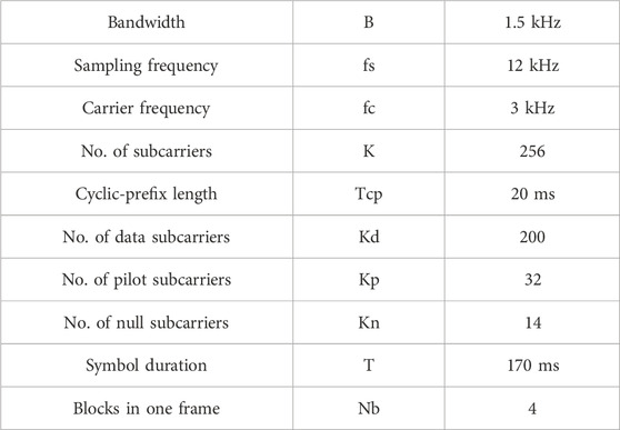
Table 4. UWA CP-OFDM settings.

We assume that the channel has 10 random paths, where the inter-arrival times are distributed exponentially with a mean of 0.5 ms, and the multipath amplitude follows Rayleigh distribution with negative exponential attenuation of average power. Each OFDM frame has four blocks, and the temporary correlation coefficients of the channel within each block are greater than 0.7. Furthermore, the data subcarriers are encoded using 1/2 non-binary low-density parity check (LDPC) code with quadrature phase shift keying (QPSK) modulation. In this section, we adopt least square (LS), OMP, and SBL algorithms to estimate the channel block-by-block, then we use the TMSBL and FTMSBL algorithms for joint estimation across four blocks in each frame, and we also model a curve of perfect channel state information (CSI) as a benchmark in BER performance. According to the path loss model (Stojanovic and Preisig, 2009):

$A\left(l,f\right)={\left(\frac{l}{l_r}\right)}^{k}a{\left(f\right)}^{l-l_r},$

where $f$ is the signal frequency and $l$ is the transmission distance, taken in reference to some $l_r$. The path loss exponent $k$ models the spreading loss. $a$ can be obtained using an empirical formula (Stojanovic and Preisig, 2009), and its usual values are between 1 and 2 (for cylindrical and spherical spreading, respectively). We set $k=1$, $a\left(f\right)=5dB/km$, and $l=2\sim 3km$. So, $A\left(l,f\right)\approx 5dB$.

The performance comparison of MSE and BER is shown in Figure 3 and Figure 4, respectively. Figure 3 shows that the MSE performance of the LS method is the worst. The performance of the SBL algorithm is better than that of the OMP algorithm but less than that of the TMSBL and FTMSBL methods. Both TMSBL and FTMSBL use four OFDM blocks for joint processing, and the MSE performance of FTMSBL is close to that of TMSBL.

Figure 3

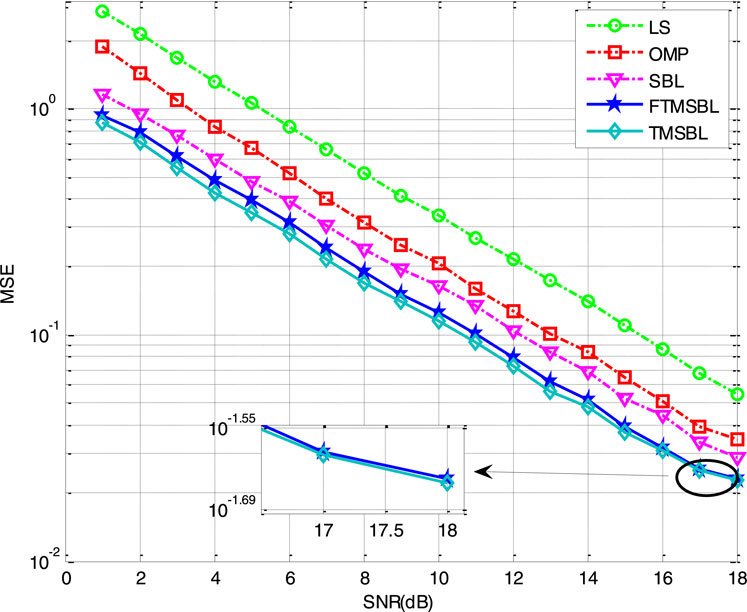
Figure 3. Comparison of MSE performance in strong temporal correlated channels.

Figure 4

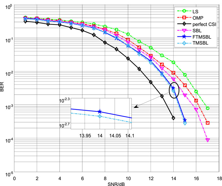
Figure 4. Comparison of decoded BER performance in strong temporal correlated channels.

Figure 4 shows that the BER performance trend of each algorithm is consistent with the MSE figure. The BER performance of the LS method is still the worst, and the OMP method outperforms the LS method by approximately 1 dB. Based on the joint estimation, the FTMSBL method achieves better performance than the OMP and SBL methods, and it is close to the TMSBL method. Meanwhile, the performance of the FTMSBL method is close to the perfect CSI curve.

In summary, the temporal joint processing uses the joint sparse structure to estimate the channel of multiple OFDM blocks at the same time. The performances of MSE and BER of the FTMSBL algorithm are similar to those of the traditional Bayesian learning algorithm TMSBL, and the computational efficiency is higher than that of the TMSBL algorithm. Considering the channel correlation in time domain of several consecutive OFDM blocks, the TMSBL and FTMSBL algorithms can not only exploit the sparse structure of channel paths but also use the temporal correlation from multiple received signals to achieve the best performance in strong temporal correlated channels.

5 Experiment results

The simulation diagram of the Qingdao sea test scenario is shown in Figure 5. In the shallow sea experiment, ship A was anchored, while ship B floated naturally on the water surface at a speed of 1.5 knots. The seawater depth is 50 m, the distance between the two ships is 2 km, and the depth of the transmitting and receiving transducer is 30 m.

Figure 5

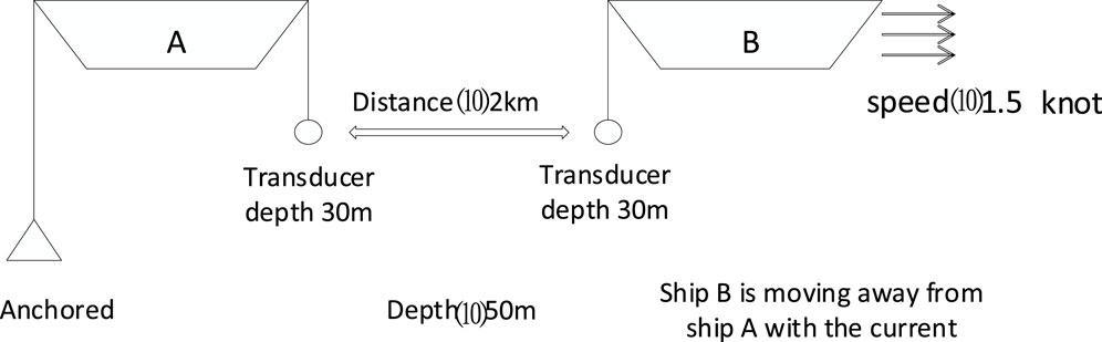
Figure 5. Schematic diagram of the distribution of the sea trial.

Simulation results show that the proposed method is effective in the UWA channel. Next, we use real experimental data to further verify the performance. The UWA CP-OFDM system settings are shown in Table 5. In the experiment, the distance between the two transducers is 2 km, and the depth of the transducer is 30 m (Figure 3). We sent 10 consecutive OFDM signal frames and set the linear frequency modulation (LFM) signal before each frame for synchronization.

Table 5

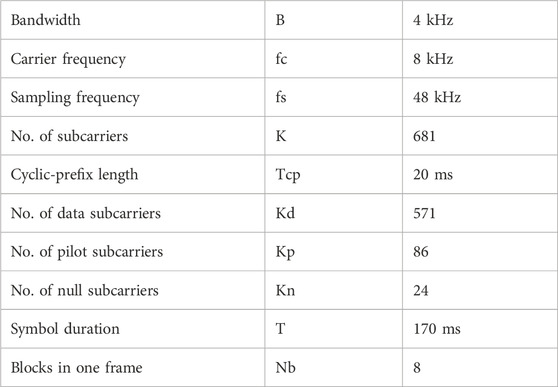
Table 5. UWA CP-OFDM settings in the sea trial.

Figure 6 shows the estimated CIR by TMSBL and the proposed methods for the first block. In addition, we also provide a rough estimate of CIR based on the correlation between the received LFM signal and the local template. The results show that the channel is sparse, which has multiple effective paths, and the total delay spread is approximately 20 ms. The channel impulse responses estimated by the two joint estimation methods are very similar in terms of delay and amplitude.

Figure 6

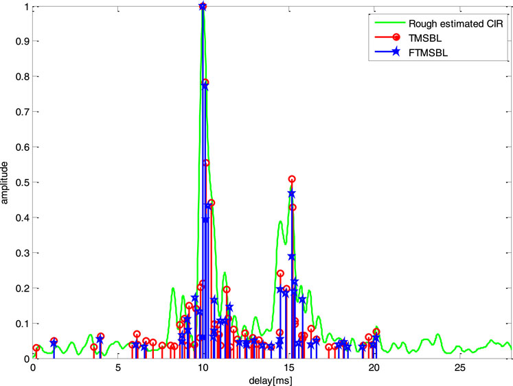
Figure 6. Estimated CIR in the sea trial.

Figure 7 shows the performance comparison of different algorithms in sea trials. The BER of the TMSBL method is still the lowest, followed closely by that of FTMSBL. In frames 5, 7, 9, and 10, the performance advantage of TMSBL and FTMSBL over SBL and OMP is clearly seen. In addition, in frames 1 and 3, the performance of the four algorithms is close. Then, we combine this BER result with channel parameters for analysis.

Figure 7

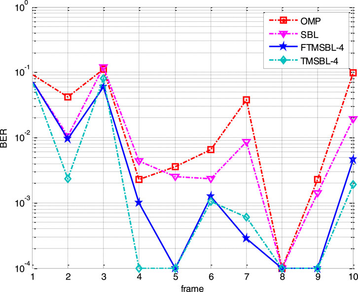
Figure 7. Comparison of decoded BER performance in the sea trial.

Figure 8 shows the temporal correlation coefficients between different blocks in the 6-frame OFDM signal. We adopted FTMSBL-4 and TMSBL-4 algorithms, where four blocks were used as a group (the first four blocks and the back four blocks) to jointly estimate channel impulse response. Then, we calculated the temporal correlation coefficients of four blocks within one group, respectively. We can find that the temporal coefficients of most blocks in frames 5, 7, 9, and 10 are above 0.5, which corresponds to the low bit error rate of FTMSBL and TMSBL in Figure 7. The temporal coefficients of frames 1 and 3 are mostly less than 0.5, and FTMSBL also shows good performance in the time-varying channel, which has a close recovery to TMSBL.

Figure 8

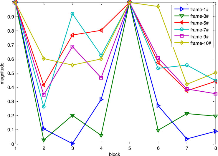
Figure 8. Temporal correlation coefficients in the sea trial.

6 Conclusion

In this paper, we propose a fast temporal multiple sparse Bayesian learning-based channel estimation method for the UWA OFDM system. Compared with the TMSBL algorithm, the FTMSBL algorithm improves computational efficiency. At the same time, the channel estimation performance of the time-domain joint FTMSBL algorithm has a close recovery performance to that of TMSBL. Compared with the SBL and OMP algorithms of block-by-block, FTMSBL improves the accuracy of sparse channel estimation and demonstrates good performance and strong robustness in time-varying channel estimation. In addition, the algorithm has low computational complexity, which helps save running time.

Data availability statement

The original contributions presented in the study are included in the article/Supplementary Material; further inquiries can be directed to the corresponding author.

Author contributions

SZ: methodology, resources, writing–original draft. SJ: writing–original draft and software. XZ: writing–original draft, formal analysis, and investigation. BL: writing–review and editing and validation.

Funding

The author(s) declare that financial support was received for the research, authorship, and/or publication of this article. This work was supported by the National Key R&D Program of China under Grant No. 2021YFC3100900.

Conflict of interest

The authors declare that the research was conducted in the absence of any commercial or financial relationships that could be construed as a potential conflict of interest.

Publisher’s note

All claims expressed in this article are solely those of the authors and do not necessarily represent those of their affiliated organizations, or those of the publisher, the editors, and the reviewers. Any product that may be evaluated in this article, or claim that may be made by its manufacturer, is not guaranteed or endorsed by the publisher.

References

Berger, C., Zhou, S., Preisig, J., and Willett, P. (2010). Sparse Channel estimation for multicarrier underwater acoustic communication: from subspace methods to compressed sensing. IEEE J. Trans. Signal Process. 58 (3), 1708–1721. doi:10.1109/TSP.2009.2038424

CrossRef Full Text | Google Scholar

Cawley, G., and Nicola, L. C. (2007). Preventing over-fitting during model selection via Bayesian regularisation of the hyper-parameters. J. Mach. Learn. Res. 8 (8), 841–861.

Google Scholar

Cho, Y. H. (2022). Fast Sparse Bayesian learning-based channel estimation for underwater acoustic OFDM systems. Appl. Sci. 12 (19), 10175. doi:10.3390/app121910175

CrossRef Full Text | Google Scholar

Feng, X., Wang, J., Sun, H., Qi, J., Qasem, Z. A., and Cui, Y. (2023). Channel estimation for underwater acoustic OFDM communications via temporal sparse Bayesian learning. Signal Process. 207, 108951. doi:10.1016/j.sigpro.2023.108951

CrossRef Full Text | Google Scholar

Guo, W., Li, C., Lei, D., and Wang, W. (2014). Joint sparse model based OFDM compressed sensing channel estimation. J. Beijing Univ. Posts Telecom. 37 (3), 1–6. doi:10.13190/j.jbupt.2014.03.001

CrossRef Full Text | Google Scholar

Guyon, I., Saffari, A., Dror, G., and Cawley, G. (2010). Model selection: beyond the bayesian/frequentist divide. J. Mach. Learn. Res. 11 (1), 61–87.

Google Scholar

Huang, J., Berger, C. R., Zhou, S., and Huang, J. (2010). “Comparison of basis pursuit algorithms for sparse channel estimation in underwater acoustic OFDM,” in 2010 IEEE international conference on oceans (Sydney, Australia). June 575–578, 2010.

CrossRef Full Text | Google Scholar

Huang, S., Yang, T., and Huang, C. (2013). Multipath correlations in underwater acoustic communication channels. J. Acoust. Soc. Am. 133 (4), 2180–2190. doi:10.1121/1.4792151

PubMed Abstract | CrossRef Full Text | Google Scholar

Jia, S., Zou, S., Zhang, X., and Da, L. (2022). Multi-block Sparse Bayesian learning channel estimation for OFDM underwater acoustic communication based on fractional Fourier transform. ’’ J. Appl. Acoust. 192, 108721. doi:10.1016/j.apacoust.2022.108721

CrossRef Full Text | Google Scholar

Li, B., Zhou, S., Stojanovic, M., Freitag, L., and Willett, P. (2008). Multicarrier communication over underwater acoustic channels with nonuniform Doppler shifts. IEEE J. Ocean. Eng. 33 (2), 198–209. doi:10.1109/JOE.2008.920471

CrossRef Full Text | Google Scholar

Ma, L., Qiao, G., and Liu, S. (2015). A combined Doppler scale estimation scheme for underwater acoustic OFDM system. J. Comput. Acoust. 23 (4), 1540004. doi:10.1142/s0218396x15400044

CrossRef Full Text | Google Scholar

Mason, S., Berger, C., Zhou, S., and Willett, P. (2008). Detection, synchronization, and Doppler scale estimation with multicarrier waveforms in underwater acoustic communication. IEEE J. Sel. Areas Commun. 26 (9), 1638–1649. doi:10.1109/jsac.2008.081204

CrossRef Full Text | Google Scholar

Naoumi, S., Bazzi, A., Bomfin, R., and Chafii, M. (2024). Complex neural network based joint AoA and AoD estimation for bistatic ISAC. IEEE J. Sel. Top. Signal Process., 1–15. doi:10.1109/jstsp.2024.3387299

CrossRef Full Text | Google Scholar

Prasad, R., Murthy, C. R., and Rao, B. D. (2014). Joint approximately sparse channel estimation and data detection in OFDM systems using sparse Bayesian learning. IEEE J. Trans. Signal Process 62 (14), 3591–3603. doi:10.1109/tsp.2014.2329272

CrossRef Full Text | Google Scholar

Qarabaqi, P., and Stojanovic, M. (2013). Statistical characterization and computationally efficient modeling of a class of underwater acoustic communication channels. IEEE J. Ocean. Eng. 38 (4), 701–717. doi:10.1109/joe.2013.2278787

CrossRef Full Text | Google Scholar

Qiao, G., Song, Q., Ma, L., Sun, Z., Liu, S., and Gan, S. (2018). Sparse bayesian learning for channel estimation in time-varying underwater acoustic OFDM communication. IEEE Access. 6, 56675–56684. doi:10.1109/access.2018.2873406

CrossRef Full Text | Google Scholar

Qiao, G., Song, Q., Ma, L., Sun, Z., and Zhang, J. (2020). Channel prediction based temporal multiple sparse bayesian learning for Channel estimation in fast time-varying underwater acoustic OFDM communications. J. Signal Process. 175 (2), 107668. doi:10.1016/j.sigpro.2020.107668

CrossRef Full Text | Google Scholar

Qiao, G., Song, Q., Ma, L., and Wan, L. (2019). A low-complexity orthogonal matching pursuit based channel estimation method for time-varying underwater acoustic OFDM systems. J. Appl. Acoust. 148 (2), 246–250. doi:10.1016/j.apacoust.2018.12.026

CrossRef Full Text | Google Scholar

Stojanovic, M., and Preisig, J. (2009). Underwater acoustic communication channels: propagation models and statistical characterization. IEEE Commun. Mag. 47 (1), 84–89. doi:10.1109/mcom.2009.4752682

CrossRef Full Text | Google Scholar

Tan, Y., Xu, W., He, Z., Tian, B., and Wang, D. (2011). “MIMO-OFDM channel estimation based on distributed compressed sensing and Kalman filter,” in IEEE international conference on signal processing, communications and computing, xi'an, China. June 1–4, 2011.

Google Scholar

Tipping, M. E. (2001). Sparse bayesian learning and the relevance vector machine. J. Mach. Learn. Res. 1, 211–244.

Google Scholar

Wang, C., Yin, J., Huang, D., and Zielinski, A. (2015). Experimental demonstration of differential OFDM underwater acoustic communication with acoustic vector sensor. J. Appl. Acoust. 91, 1–5. doi:10.1016/j.apacoust.2014.11.013

CrossRef Full Text | Google Scholar

Wang, S., Liu, M., and Li, D. (2021). Bayesian learning-based clustered-sparse channel estimation for time-varying underwater acoustic OFDM communication. Sensors 21 (14), 4889. doi:10.3390/s21144889

PubMed Abstract | CrossRef Full Text | Google Scholar

Zhang, Z., and Rao, B. D. (2011). Sparse signal recovery with temporally correlated source vectors using sparse Bayesian learning. IEEE J. Sel. Top. Signal Process 5 (5), 912–926. doi:10.1109/jstsp.2011.2159773

CrossRef Full Text | Google Scholar

Zhou, Y., Tong, F., and Zhang, G. (2017). Distributed compressed sensing estimation of underwater acoustic OFDM channel. J. Appl. Acoust. 117, 160–166. doi:10.1016/j.apacoust.2016.10.021

CrossRef Full Text | Google Scholar