Abstract
As one of the important statistical methods, quantile regression (QR) extends traditional regression analysis. In QR, various quantiles of the response variable are modeled as linear functions of the predictors, allowing for a more flexible analysis of how the predictors affect different parts of the response variable distribution. QR offers several advantages over standard linear regression due to its focus on estimating conditional quantiles rather than the conditional mean of the response variable. This paper investigates QR over sensor networks, where each node has access to a local dataset and collaboratively estimates a global QR model. QR solves a non-smooth optimization problem characterized by a piecewise linear loss function, commonly known as the check function. We reformulate this non-smooth optimization problem as the task of finding a saddle point of a convex–concave objective and develop a distributed primal–dual hybrid gradient (dPDHG) algorithm for this purpose. Theoretical analyses guarantee the convergence of the proposed algorithm under mild assumptions, while experimental results show that the dPDHG algorithm converges significantly faster than subgradient-based schemes.
1 Introduction
Distributed signal processing (Hovine and Bertrand, 2024; Cattivelli and Sayed, 2010; Schizas et al., 2009) in wireless sensor networks addresses the challenges of limited energy, processing power, and communication range of individual sensors. By applying collaborative computational algorithms, sensors can operate as a distributed signal processor, overcoming individual limitations and improving energy efficiency. Distributed signal processing is particularly used in various applications where distributed algorithms can enhance the power efficiency by avoiding data centralization, including environmental monitoring, healthcare, and military surveillance. However, the complexity of real-world sensor data often involves non-linear relationships, heteroscedasticity, and outliers. In such environments, traditional distributed methods like least squares regression may fail to provide robust estimates due to the influence of extreme values or noise.
Quantile regression (QR) (Waldmann, 2018) offers a solution by estimating conditional quantiles of the data distribution, rather than just the mean, making it more robust to outliers and better suited for modeling heterogeneous data sources. Quantile regression has gained significant attention as a robust approach to regression analysis, particularly in situations where the distribution of the response variable is not symmetric or when outliers are present, and has applications in various fields, including ecology, economics, and industry (Cade and Noon, 2003; Ben Taieb et al., 2016; Wan et al., 2017). Some efficient numerical methods, including alternating direction method of multipliers (ADMM) (Mirzaeifard et al., 2024; Bazzi and Chafii, 2023), majorize–minimize (MM) (Kai et al., 2023; Cheng and Kuk, 2024), and machine learning (Patidar et al., 2023; Hüttel et al., 2022), were used for solving the optimization problem associated with quantile regression. Recent research has focused on distributed quantile regression (dQR) in sensor networks. In distributed sensor networks, where data from different sensors can vary significantly in terms of noise and variability, quantile regression can be applied at the local level to estimate the distributional characteristics of the data at each sensor node. Wang and Li (2018) proposed a diffusion-based distributed strategy [including a variant for sparse models (Bazzi et al., 2017)] for quantile regression over wireless sensor networks. Wang and Lian (2023), Lee et al. (2018), and Lee et al. (2020) introduced several consensus-based dQR methods for sensor networks. These methods overcome challenges in distributed settings, including limited storage and transmission power, while maintaining statistical robustness. They offer promising solutions for quantile-based analyses in decentralized sensor networks across diverse applications.
It should be noted that quantile regression involves a non-differentiable optimization problem with a piecewise linear loss function, also known as the check function. Most existing quantile regression algorithms rely on subgradient methods, which typically exhibit sublinear convergence rates. Although these methods have certain merits, they often struggle with slow convergence when tackling the non-differentiability of the optimization problem. Alternatively, techniques such as MM (Kai et al., 2023; Cheng and Kuk, 2024) mitigate the non-differentiability issue by minimizing a smooth majorizer of the check function instead of the function itself. However, these methods can introduce additional computational complexity and may not fully exploit the structure of distributed settings. As a data-driven approach, the machine learning-based methods (Patidar et al., 2023; Hüttel et al., 2022; Delamou et al., 2023; Njima et al., 2022) can circumvent the non-differentiability issue. However, it relies heavily on the availability of large datasets, which may not always be feasible or efficient in certain scenarios.
In this paper, we propose a novel approach for diffusion-based distributed quantile regression, leveraging the primal–dual hybrid gradient method to find a saddle point of a convex–concave objective. This strategy accelerates convergence and significantly enhances the efficiency of the quantile regression process.
2 Network model and problem formulation
2.1 Preliminaries
In this section, we present a brief introduction to quantile regression. Let be a scalar random variable, a -dimensional random vector, and represent the conditional cumulative distribution function. The conditional quantile is defined as follows:for . A linear model is given by , where is the input data vector, is the deterministic unknown parameter vector of interest, and is the observed noise following a certain distribution. Unlike standard regression methods, which focus on estimating the mean of , quantile regression provides a more comprehensive analysis by modeling different points (quantiles) in the distribution of .
In the quantile regression model, is assumed to be linearly related to as follows: where represents the -th quantile of the noise. The -th quantile of the noise, , is not necessarily 0 (e.g., for asymmetric noise distributions). Explicitly including avoids the restrictive assumption that , thereby allowing the model to flexibly adapt to the true noise distribution. Omitting would force the conditional quantile to pass through the origin, which is often inappropriate in real-world applications. Since both and are unknown parameters that must be estimated, the optimization problem for estimating and can be expressed as follows:Here, is the non-differentiable quantile loss function, also known as the check function, defined as follows:This function adjusts the loss asymmetrically depending on whether the residual is positive or negative, allowing the model to estimate conditional quantiles for different values.
2.2 Network model and problem formulation
Consider a network consisting of nodes distributed over a certain geographic region. Assume that the network is strongly connected, that is, there is no isolated node in the network. Every node has access to the realization of zero-mean random data at every time instant and is allowed to communicate only with its neighbors , where is a scalar measurement, is an measurement vector, and denotes a set of nodes in the neighborhood of node including itself. Moreover, satisfy a standard lineal regression modelwhere is the measurement noise and is a deterministic sparse vector of dimension .
The aim of this study is to develop a distributed quantile regression algorithm to estimate using the dataset . Recalling Equation 1, the sparsity-penalized quantile regression estimate of is obtained by minimizing the global cost function for quantile regression across the network, formulated as follows:whereHere, represents the global cost function over the network, and the local cost functions , which reflect the costs at each node , are aggregated to form the global objective. The first term in Equation 4 captures the quantile regression residuals across all nodes and data points , while the second term imposes -norm regularization on , encouraging sparsity. In this formulation, is the augmented input data vector, is the augmented parameter vector to be estimated, and is a weighting matrix with individual entries . The coefficients are non-negative weighting factors, satisfyingThis condition (Equation 5) is explicitly satisfied by widely used weight rules in the distributed optimization literature (Cattivelli and Sayed, 2010; Tu and Sayed, 2011). In addition, is a regularization parameter controlling the sparsity of the solution, and denotes the -norm which encourages sparse solutions.
We assume that the underlying network operates under ideal and stable communication conditions. Transient link or node failures—well-studied in the distributed network literature (Gao et al., 2022; Swain et al., 2018)—are effectively handled using established engineering solutions, such as fault-tolerant protocols, redundancy, and consensus mechanisms, thereby ensuring system reliability.
3 Distributed primal–dual hybrid gradient algorithm
This section first introduces a distributed quantile regression framework and formulates our problem as a saddle-point optimization problem. Subsequently, a distributed primal–dual hybrid gradient algorithm (dPDHG) for quantile regression is proposed, and its convergence is analyzed.
3.1 Diffusion-based distributed estimation framework
Since the main task of quantile regression is to estimate the parameter vector , we introduce a diffusion-based distributed estimation framework. In this framework, each node solves its local optimization problem using the subsequently proposed algorithm. The nodes then share their intermediate results with neighboring nodes to collaboratively solve the global quantile regression problem.
By definition in Equation 4, the local cost function of node can be further expressed as a combination of the local cost functions of its neighboring nodes, i.e., with . Therefore, each node obtains its estimate by combining its newly generated estimate with the estimates received from its neighboring nodes:
Based on this idea, we will use a distributed strategy in the following subsections to solve the problem (Equation 3).
This study focuses on a diffusion-based framework for decentralized quantile regression. The integration of consensus-based strategies with primal–dual hybrid gradient methods for distributed quantile regression, which presents significant algorithmic challenges, is left for future investigation.
3.2 Dual problem and saddle point optimization
By definition, we split into with and . For the local optimization problem , the check function is not differentiable at the origin. To address this, we adopt its conjugate function , which allows us to express the problem equivalently. The conjugate function is defined asUsing the conjugate function , we can express asThis suggests that can be expressed aswhere , , , and is an indicator function given byWe can obtain a dual problem associated with the original function minimization problem , which can be expressed as follows:
This indicates that the global optimization problem (Equation 3) can be formulated aswhich has a standard saddle-point optimization problem expression with the primal variable and the dual variable , where . Note that we are primarily concerned with the first elements of the vector , which can be interpreted as the estimate of . Moreover, is defined as .
3.3 Algorithmic principles and derivations of the dPDHG
This section presents the algorithmic principles and derivations of the proposed dPDHG to solve
Equation 9. Its basic framework includes the following steps (a)–(d), which involve iterative updates of the primal and dual variables
:
(a) Update the primal variable , :
where
is an element-wise proximal operator defined by
. It is readily deduced that
with
being the
-th element of
.
(b) Update the auxiliary variable , :
(c) Each node combines its newly generated estimate with the estimates received from its neighboring nodes, : .
(d) Update the dual variable , :
where one can deduce that the proximal operator
projects
onto the interval
element-wise:
.
(e) Assign global to local for the next iteration.
The algorithm continues iterating until the stopping criterion is met, typically based on the difference between successive iterates or the duality gap. Finally, we summarize the proposed dPDHG algorithm in Table 1.
TABLE 1
| Input: |
| 1: Initialize: |
| 2: fordo |
| 3: fordo |
| 4: |
| 5: |
| 6: end for |
| 7: fordo |
| 8: |
| 9: |
| 10: end for |
| 11: end for |
dPDHG.
3.4 Selection of the primal–dual step sizes
In the above steps, are the primal–dual step sizes chosen to ensure the convergence of the dPDHG algorithm. For the standard form of a convex–concave saddle-point optimization problem , the step sizes chosen to ensure convergence of the PDHG algorithm are required (Esser et al., 2010), where . For the problem (Equation 9) mentioned in this paper, can be treated as , , and , respectively.
Note that, for each , choosing a small and large results in small dual residual but large primal residual , and vice versa, wherewhere and . Therefore, adaptive strategies—such as those proposed in Goldstein et al. (2015); Chambolle et al. (2024)—can also be employed to balance the progress between the primal and dual updates, thereby enhancing the convergence. If the primal residual is sufficiently large compared to the dual residual , for example , we increase the primal step size by a factor of and decrease the dual stepsize by a factor of . If the primal residual is somewhat smaller than the dual residual, we do the opposite. If both residuals are comparable in size, then let the step sizes remain the same on the next iteration. Moreover, when we modify the step size as the iteration continues, we also shrink the adaptivity level to , for .
4 Simulation examples
We consider a connected network with nodes that are positioned randomly on a unit square area, with a maximum communication distance of 0.4 unit length. The three non-zero components of the sparse vector having size are set as 1.0 with their positions randomly selected, while the others are zeros. The weighting matrix in Equation 5 is chosen according to the metropolis criterion (Cattivelli and Sayed, 2010; Tu and Sayed, 2011), that is,where denotes the degree of node (the cardinality of its closed neighborhood).
We begin by evaluating the performance of the distribution estimation for . The regressors, , , and , are modeled as independent, zero-mean Gaussian random variables in both time and space. Their covariance matrices are assumed to be identity matrices. Moreover, we consider three types of noise : one following the beta distribution and two following heavy-tailed distributions. Specifically, the heavy-tailed noises are generated from Student’s t-distribution with 2 degrees of freedom (dof) and the Cauchy distribution. Beta-distributed noise is produced using the MATLAB command , which maps the standard beta-distributed values from [0,1] to . The Student’s t-distributed noise is generated using , and the Cauchy-distributed noise is generated via the transformation: where, for each time step and each node , a uniform random number in [0,1] is first drawn using , shifted to the interval , and then transformed using to yield a Cauchy-distributed sample.
Figures 1–3 illustrate the transient-network mean-square deviation (MSD) performance of our proposed dPDHG algorithm, compared with three benchmark algorithms: the subgradient-based algorithm (Subgrad) (Wang and Li, 2018), the majorization–minimization algorithm (MM) (Kai et al., 2023), accelerated proximal-based gradient methods(APG) (Chen and Ozdaglar, 2012), and the least mean squares (LMS) algorithm (Liu et al., 2012). The transient network MSD is defined as , and the results are presented for different quantile levels, ; Figures 1–3 are presented under the presence of beta-distributed noise, -distributed noise, and Cauchy noise, respectively.
FIGURE 1
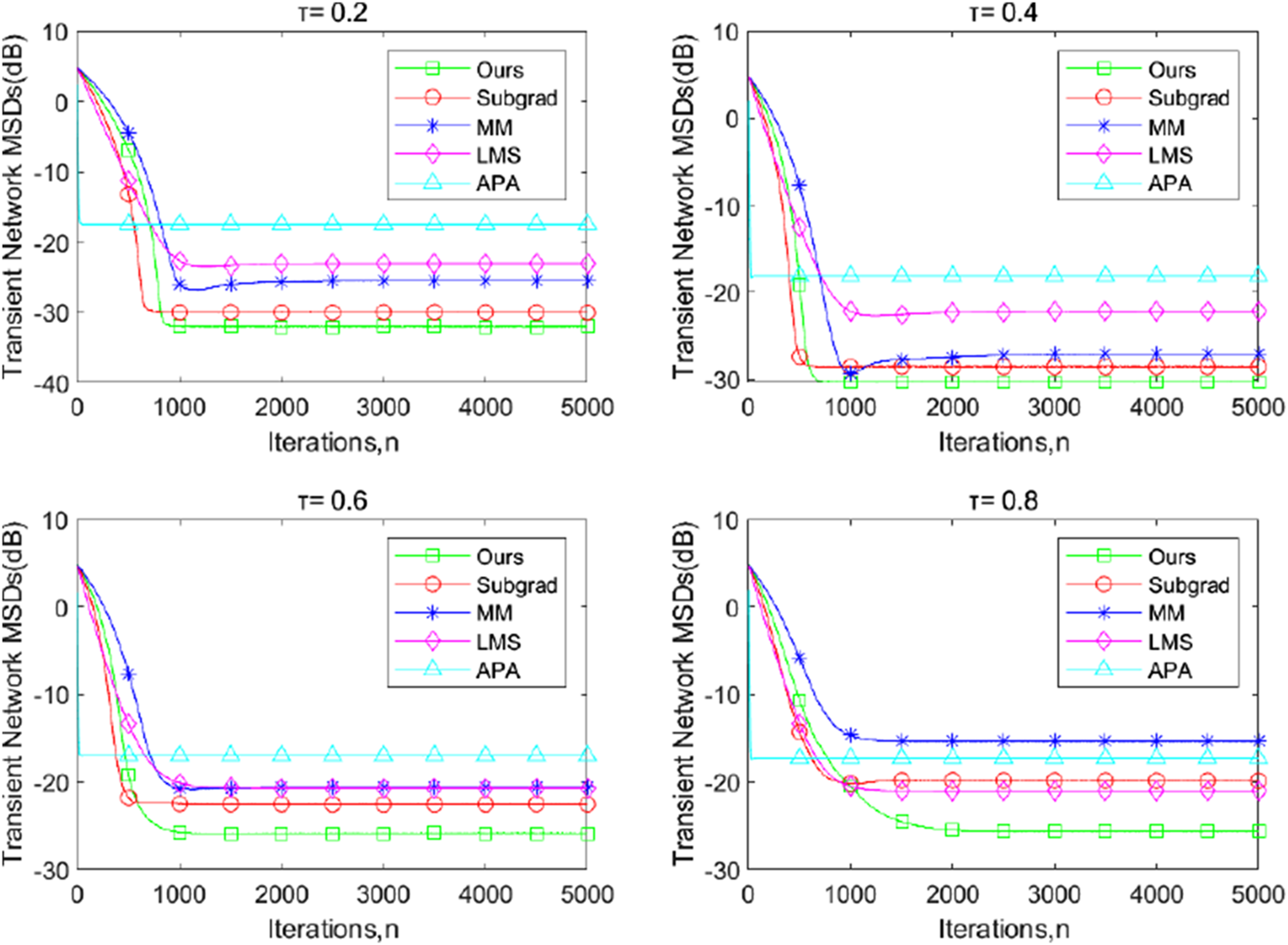
The transient network MSDs of the proposed dPDHG algorithm compared with three benchmark distributed algorithms: the Subgrad, the MM, and the LMS, and the APA algorithms for estimating , where is the beta-distributed noise.
FIGURE 2
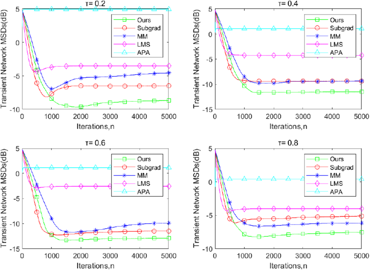
The transient-network MSDs of the proposed dPDHG algorithm compared with three benchmark distributed algorithms: the Subgrad, the MM, and the LMS, and the APA algorithms for estimating , where is the t-distribution noise.
FIGURE 3
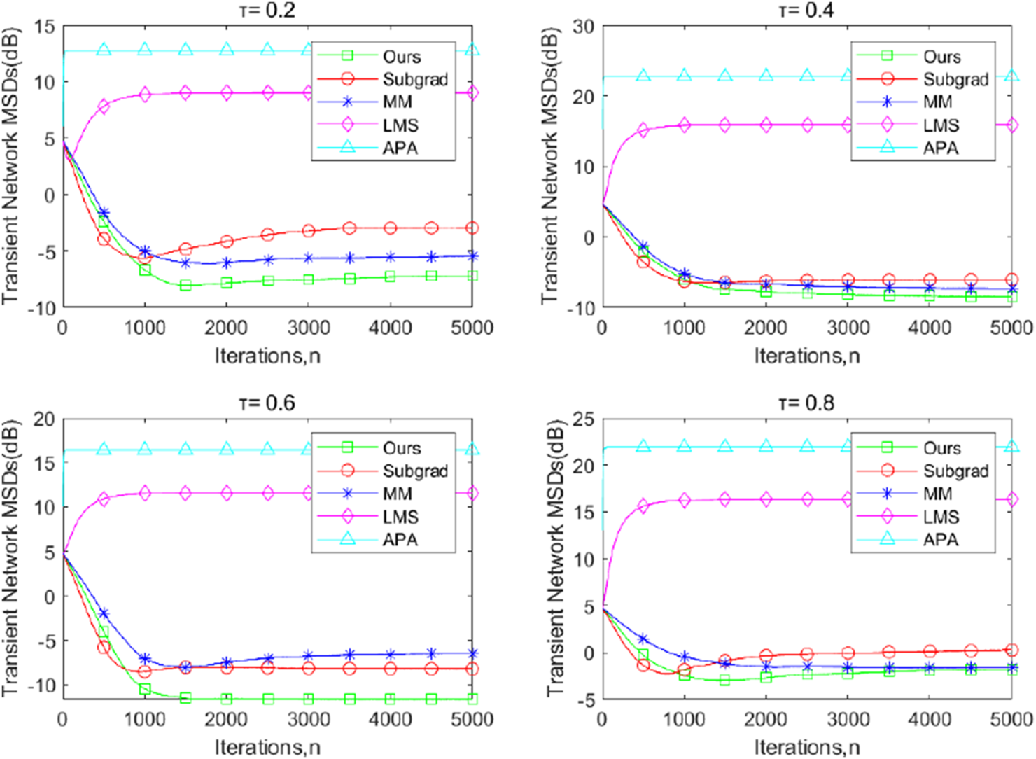
The transient network MSDs of the proposed dPDHG algorithm compared with three benchmark distributed algorithms: the Subgrad, the MM, and the LMS, and the APA algorithms for estimating , where is the Cauchy noise.
Across all quantile levels, our algorithm demonstrates superior convergence properties, achieving the lowest MSD values at steady state, compared to the other algorithms. The APG and LMS algorithms exhibit the highest MSD, indicating poor adaptation to the beta-distributed noise, -distributed noise, and the Cauchy noise. The MM algorithm outperforms Subgrad but converges to higher MSD values than our approach. Subgrad shows moderate performance but struggles to maintain consistent improvements across iterations. These results highlight the robustness and efficiency of the proposed DQR algorithm in addressing distributed quantile regression tasks.
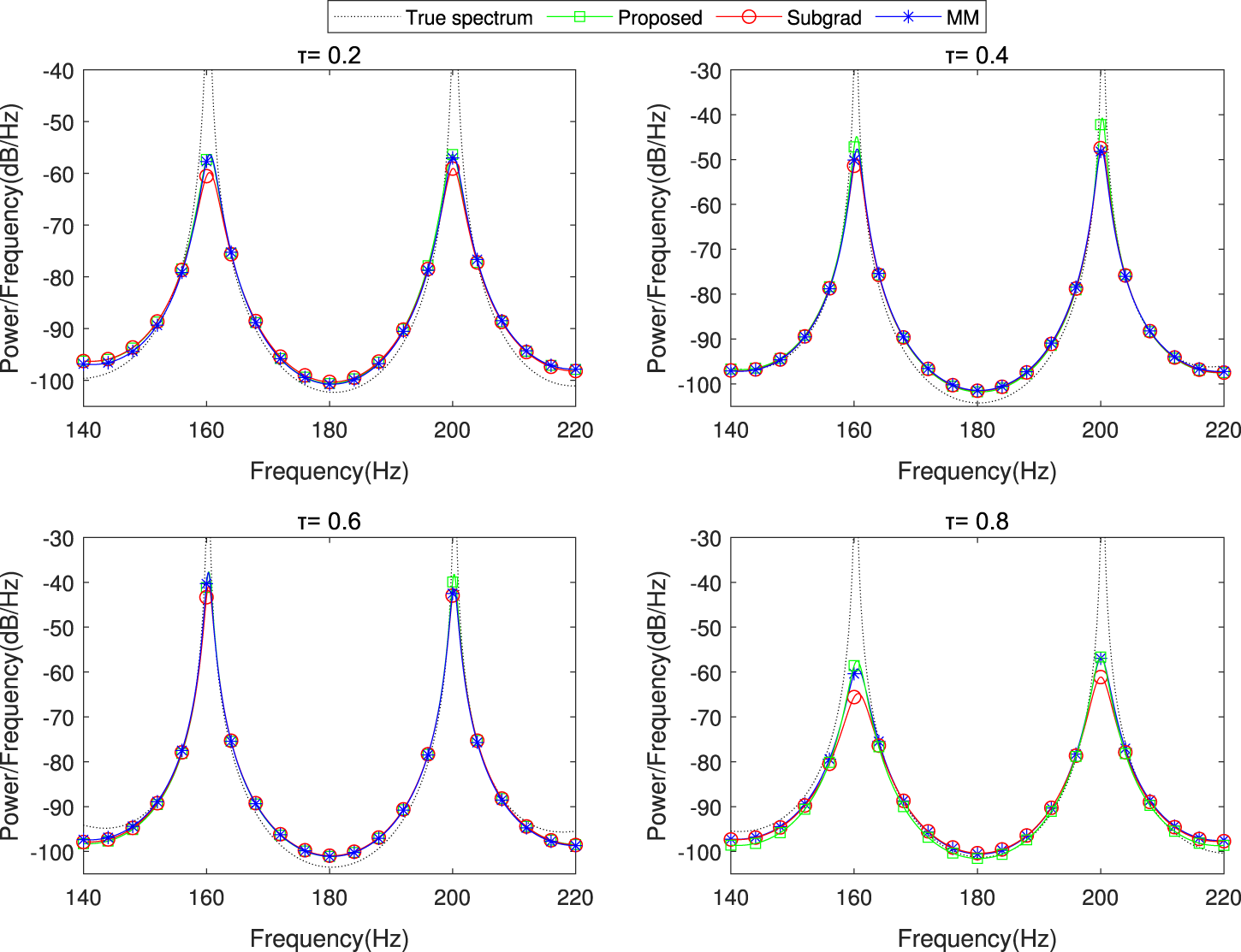
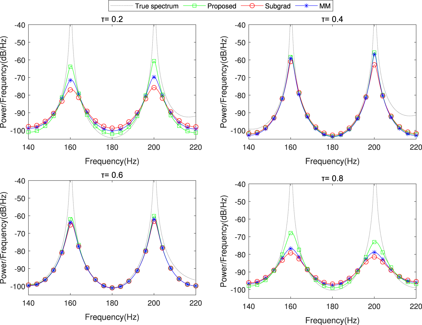
We further consider a practical application in spectrum estimation for a narrow-band source. A peaky spectrum can be modeled by an -order sparse AR process (Liu et al., 2012; Schizas et al., 2009): where is a noise and are the AR coefficients. The source propagates to sensor via a transmission channel modeled by a -order FIR filter, yielding an observation where is an additive sensing noise and are the FIR coefficients. It is readily deduced that can be rewritten as an autoregressive moving average (ARMA) process (see Appendix A):where the MA coefficients and the variance of the white noise depend on and the variances of the noise terms and . For more details, refer to Appendix A. To determine the spectral contents of the source, the MA term in Equation 11 can be treated as an observation noise, and then the spectral peaks of the source can be obtained by estimating the AR coefficients . By letting and , the problem of spectrum estimation fits our model (Equation 2) and becomes that of the distributed estimation as mentioned above.
–
6compare the true source spectrum with the estimated results averaged across
nodes under three distinct channel noise distributions: beta-distributed, t-distributed, and Cauchy noise
. The noise sequences are generated using the methodology outlined previously, maintaining consistent simulation parameters. In this simulation, we configure the AR coefficients and channel parameters as follows:
The peaked spectrum is generated from a 20th-order autoregressive (AR) model (order ). The true spectral peaks are located at normalized frequencies corresponding to 160 Hz and 200 Hz.
The multipath channels have a fixed length of for all .
The FIR channel coefficients are generated using the randn(2,1) command in MATLAB, producing standard normal random values.
The AR process noise is modeled as zero-mean Gaussian random variables with variance .
FIGURE 4
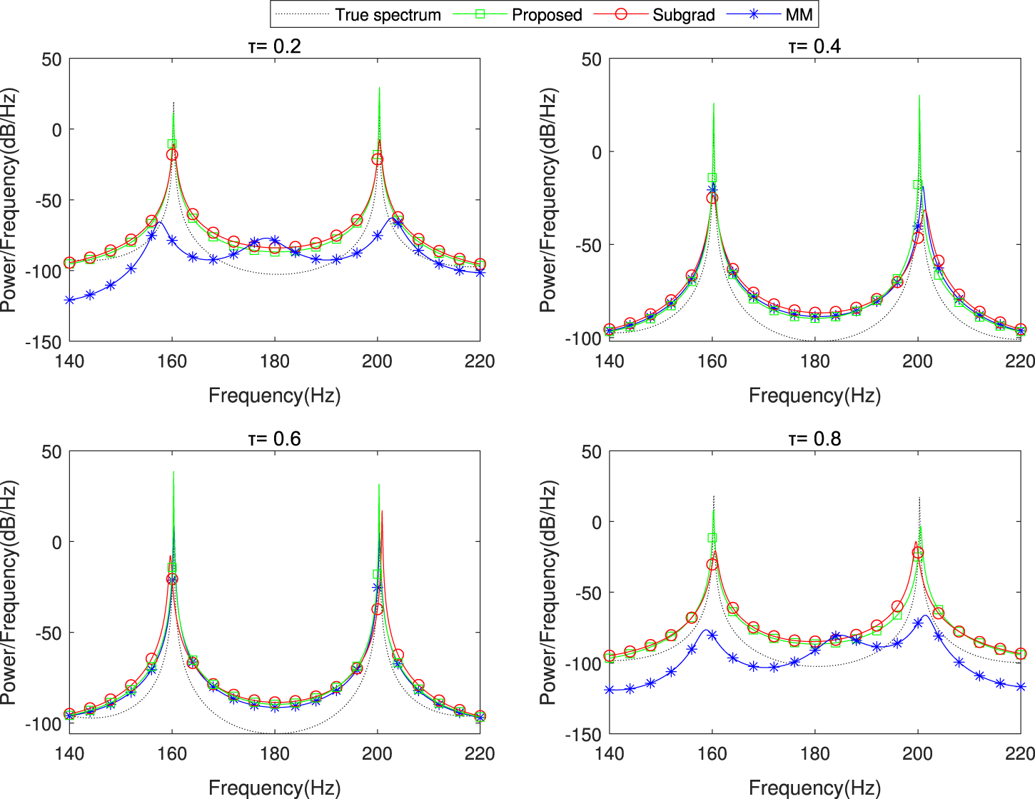
The spectrum estimation results of the proposed dPDHG algorithm compared with two benchmark distributed algorithms: Subgrad and MM. The comparison is conducted in the presence of beta-distributed noise .
FIGURE 5
The spectrum estimation results of the proposed dPDHG algorithm compared with two benchmark distributed algorithms: Subgrad and MM. The comparison is conducted in the presence of t-distributed noise .
FIGURE 6
The spectrum estimation results of the proposed dPDHG algorithm compared with two benchmark distributed algorithms: Subgrad and MM. The comparison is conducted in the presence of Cauchy noise .
As shown in these figures, our algorithm closely matches the true spectrum across all tested quantile levels, achieving higher estimation accuracy than the benchmark algorithms. These results highlight the robustness and precision of the proposed dPDHG algorithm in estimating the spectrum of narrow-band sources under challenging noise conditions.
5 Conclusion
This paper investigated distributed robust estimation in sensor networks and introduced a distributed quantile regression algorithm based on the primal–dual hybrid gradient method. The proposed algorithm effectively addresses the challenge of non-differentiability in the optimization problem by iteratively identifying the saddle point of a convex–concave objective. Additionally, it mitigates the issue of slow convergence commonly associated with such problems. The method demonstrates robustness, scalability, and suitability for processing large-scale data distributed across sensor networks.
Statements
Data availability statement
The raw data supporting the conclusions of this article will be made available by the authors, without undue reservation.
Author contributions
ZQ: Writing – review and editing. ZL: Writing – original draft.
Funding
The author(s) declare that no financial support was received for the research and/or publication of this article.
Conflict of interest
The authors declare that the research was conducted in the absence of any commercial or financial relationships that could be construed as a potential conflict of interest.
Generative AI statement
The author(s) declare that no Generative AI was used in the creation of this manuscript.
Publisher’s note
All claims expressed in this article are solely those of the authors and do not necessarily represent those of their affiliated organizations, or those of the publisher, the editors and the reviewers. Any product that may be evaluated in this article, or claim that may be made by its manufacturer, is not guaranteed or endorsed by the publisher.
References
1
Bazzi A. Chafii M. (2023). On integrated sensing and communication waveforms with tunable papr. IEEE Trans. Wirel. Commun.22, 7345–7360. 10.1109/TWC.2023.3250263
2
Bazzi A. Slock D. T. M. Meilhac L. (2017). “A Newton-type forward backward greedy method for multi-snapshot compressed sensing,” in 2017 51st asilomar conference on signals, systems, and computers, 1178–1182. 10.1109/ACSSC.2017.8335537
3
Ben Taieb S. Huser R. Hyndman R. J. Genton M. G. (2016). Forecasting uncertainty in electricity smart meter data by boosting additive quantile regression. IEEE Trans. Smart Grid7, 2448–2455. 10.1109/TSG.2016.2527820
4
Cade B. S. Noon B. R. (2003). A gentle introduction to quantile regression for ecologists. Front. Ecol. Environ.1, 412–420. 10.1890/1540-9295(2003)001[0412:agitqr]2.0.co;2
5
Cattivelli F. S. Sayed A. H. (2010). Diffusion LMS strategies for distributed estimation. IEEE Trans. Signal Process.58, 1035–1048. 10.1109/tsp.2009.2033729
6
Chambolle A. Delplancke C. Ehrhardt M. J. Schönlieb C.-B. Tang J. (2024). Stochastic primal–dual hybrid gradient algorithm with adaptive step sizes. J. Math. Imaging Vis.66, 294–313. 10.1007/s10851-024-01174-1
7
Chen A. I. Ozdaglar A. (2012). “A fast distributed proximal-gradient method,” in 2012 50th annual allerton Conference on communication, control, and computing (allerton) (IEEE).
8
Cheng Y. Kuk A. Y. C. (2024). MM algorithms for statistical estimation in quantile regression
9
Delamou M. Bazzi A. Chafii M. Amhoud E. M. (2023). “Deep learning-based estimation for multitarget radar detection,” in 2023 IEEE 97th vehicular technology conference (VTC2023-Spring), 1–5. 10.1109/VTC2023-Spring57618.2023.10200157
10
Esser E. Zhang X. Chan T. F. (2010). A general framework for a class of first order primal-dual algorithms for convex optimization in imaging science. SIAM J. Imaging Sci.3, 1015–1046. 10.1137/09076934x
11
Gao M. Niu Y. Sheng L. (2022). Distributed fault-tolerant state estimation for a class of nonlinear systems over sensor networks with sensor faults and random link failures. IEEE Syst. J.16, 6328–6337. 10.1109/jsyst.2022.3142183
12
Goldstein T. Li M. Yuan X. (2015). “Adaptive primal-dual splitting methods for statistical learning and image processing,” in Proceedings of the 29th international conference on neural information processing systems - volume 2 (Cambridge, MA, USA: MIT Press), 2089–2097.
13
Hovine C. Bertrand A. (2024). A distributed adaptive algorithm for non-smooth spatial filtering problems in wireless sensor networks. IEEE Trans. Signal Process.72, 4682–4697. 10.1109/TSP.2024.3474168
14
Hüttel F. B. Peled I. Rodrigues F. Pereira F. C. (2022). Modeling censored mobility demand through censored quantile regression neural networks. IEEE Trans. Intelligent Transp. Syst.23, 21753–21765. 10.1109/TITS.2022.3190194
15
Kai B. Huang M. Yao W. Dong Y. (2023). Nonparametric and semiparametric quantile regression via a New MM algorithm. J. Comput. Graph. Stat.32, 1613–1623. 10.1080/10618600.2023.2184374
16
Lee J. Tepedelenlioglu C. Spanias A. (2018). Consensus-based distributed quantile estimation in sensor networks. arXiv Prepr. arXiv:1805.00154.
17
Lee J. Tepedelenlioglu C. Spanias A. Muniraju G. (2020). ngermanDistributed quantiles estimation of sensor network measurements. Int. J. Smart Secur. Technol.7, 38–61. 10.4018/ijsst.2020070103
18
Liu Y. Li C. Zhang Z. (2012). Diffusion sparse least-mean squares over networks. IEEE Trans. Signal Process.60, 4480–4485. 10.1109/tsp.2012.2198468
19
Mirzaeifard R. Venkategowda N. K. D. Gogineni V. C. Werner S. (2024). Smoothing admm for sparse-penalized quantile regression with non-convex penalties. IEEE Open J. Signal Process.5, 213–228. 10.1109/OJSP.2023.3344395
20
Njima W. Bazzi A. Chafii M. (2022). Dnn-based indoor localization under limited dataset using gans and semi-supervised learning. IEEE Access10, 69896–69909. 10.1109/ACCESS.2022.3187837
21
Patidar V. K. Wadhvani R. Shukla S. Gupta M. Gyanchandani M. (2023). “Quantile regression comprehensive in machine learning: a review,” in 2023 IEEE international students’ conference on electrical, electronics and computer science (SCEECS), 1–6. 10.1109/SCEECS57921.2023.10063026
22
Schizas I. D. Mateos G. Giannakis G. B. (2009). Distributed LMS for consensus-based in-network adaptive processing. IEEE Trans. Signal Process.57, 2365–2382. 10.1109/tsp.2009.2016226
23
Swain R. Khilar P. M. Dash T. (2018). Fault diagnosis and its prediction in wireless sensor networks using regressional learning to achieve fault tolerance. Int. J. Commun. Syst.31. 10.1002/dac.3769
24
Tu S.-Y. Sayed A. H. (2011). Mobile adaptive networks. IEEE J. Sel. Top. Signal Process.5, 649–664. 10.1109/jstsp.2011.2125943
25
Waldmann E. (2018). Quantile regression: a short story on how and why. Stat. Model.18, 203–218. 10.1177/1471082x18759142
26
Wan C. Lin J. Wang J. Song Y. Dong Z. Y. (2017). Direct quantile regression for nonparametric probabilistic forecasting of wind power generation. IEEE Trans. Power Syst.32, 2767–2778. 10.1109/TPWRS.2016.2625101
27
Wang H. Li C. (2018). Distributed quantile regression over sensor networks. IEEE Trans. Signal Inf. Process. over Netw.4, 338–348. 10.1109/TSIPN.2017.2699923
28
Wang Y. Lian H. (2023). On linear convergence of ADMM for decentralized quantile regression. IEEE Trans. Signal Process.71, 3945–3955. 10.1109/TSP.2023.3325622
Appendix
Appendix A spectrum estimation
Since is generated by an AR process, we substitute the AR model into the FIR filter equation. For each , replace it with its corresponding AR expression: Thus, the observation model becomeswhere and are defined as follows:both vectors having a length of .
Appendix Equation A.1 expresses as a combination of past observations (the AR part) and past noise (the MA part), thus forming the desired ARMA process, as shown in Equation 11.
Summary
Keywords
primal–dual, quantile regression, sensor networks, distribution estimation, robustness
Citation
Qin Z and Liu Z (2025) Distributed quantile regression over sensor networks via the primal–dual hybrid gradient algorithm. Front. Commun. Netw. 6:1604850. doi: 10.3389/frcmn.2025.1604850
Received
02 April 2025
Accepted
19 May 2025
Published
17 June 2025
Volume
6 - 2025
Edited by
Ramoni Adeogun, Aalborg University, Denmark
Reviewed by
Ahmed Aftan, Middle Technical University, Iraq
Ahmad Bazzi, New York University Abu Dhabi, United Arab Emirates
Updates
Copyright
© 2025 Qin and Liu.
This is an open-access article distributed under the terms of the Creative Commons Attribution License (CC BY). The use, distribution or reproduction in other forums is permitted, provided the original author(s) and the copyright owner(s) are credited and that the original publication in this journal is cited, in accordance with accepted academic practice. No use, distribution or reproduction is permitted which does not comply with these terms.
*Correspondence: Zhaoting Liu, liuzhaoting@163.com
Disclaimer
All claims expressed in this article are solely those of the authors and do not necessarily represent those of their affiliated organizations, or those of the publisher, the editors and the reviewers. Any product that may be evaluated in this article or claim that may be made by its manufacturer is not guaranteed or endorsed by the publisher.