Towards realistic simulation of DNA-based molecular communication networks

Next to further miniaturization, the process of self-assembly has great potential for construction, computation, and even communication at the nanoscale. DNA-based self-assembly is an especially promising candidate as it is possible to create entire nanonetworks from just DNA from already existing and comparably cheap building blocks. As wet-lab experiments are still fairly expensive and complex, and self-assembly is hard to predict, simulation tools are crucial for the rapid prototyping of new ideas. However, current self-assembly simulators mainly focus on computational and construction aspects. In this paper, we present a new model for our NetTAS simulator, kTHAM, which simulates the possible interactions of very large numbers of DNA structures simultaneously and measures the process in real-time. This allows for a much more realistic analysis of DNA-based nanonetworks as compared to what is possible with other simulators and with the other models of NetTAS.

1 Introduction

Nanonetworks are among the most promising technologies’ computer science and engineering have to offer for future developments in medicine and a number of other areas (Akyildiz et al., 2008). While they offer great potential, the ability to construct such networks is currently limited. Potential materials include modified cells or bacteria, carbon nanotubes, DNA, or entirely different approaches. Due to extensive prior research and a vast multi-domain interest, DNA is likely the most well-researched construction material of the three. As early as 1982, scientists already discovered the potential of DNA as a material for construction at the nanoscale (Seeman, 1982). As DNA self-assembles autonomously, technologies based on DNA building blocks can avoid the accuracy problems other manufacturing methods are currently facing. Not long after, DNA has also been identified as one of the most promising technologies for performing computations at the nanoscale (Paun et al., 2005).

As wet lab experiments are expensive and time-consuming, and self-assembly is hard to predict, simulation tools are crucial for the rapid prototyping of new ideas for protocols, algorithms, and applications. There is currently software for both computation and construction using DNA, but to the best of our knowledge, there is no simulator that focuses on the long-term development of self-assembly systems or a possible interpretation of certain self-assembly systems as communication networks. Widespread models such as the kinetic Tile Assembly Model kTAM usually only predict the first few seconds of a well-mixed solution of DNA building blocks and may thus assume an infinite supply of such blocks for the assembly process.

This work introduces the kinetic two-handed Tile Assembly Model kTHAM as a new model for our simulator NetTAS¹. The simulator integrates the features of well-known simulators like ISU TAS (Patitz, 2011; Winfree et al., 1998). The kTHAM module simulates many assembly processes in parallel while also analyzing possible interactions between all structures in real-time. Thus, it allows for a more realistic simulation of DNA-based nanonetworks (Lau et al., 2019).

The remainder of this paper is structured as follows: Section 2 gives a brief introduction to the world of tile assembly models as a base for DNA-based nanonetwork technology. Section 3 analyzes existing simulators, and demonstrates the benefits of a new simulation module. Section 4 gives an overview of the NetTAS models and the user interface of the software. Section 5 describes the kTHAM model of the netTAS simulator as well as the real-time aspects of the simulation. Section 6 evaluates the real-time behavior and the module, and Section 7 summarizes the paper and gives a brief outlook on future work.

2 Preliminaries for DNA-based nanonetworks

In this section, we provide a brief introduction to DNA-based nanonetworks (DNN) that is necessary to understand the kTHAM. A more detailed introduction to the topic can be found in (Patitz, 2014; Lau et al., 2019), as such lengthy definitions are beyond the scope of this paper.

Self-assembly systems have DNA tiles as their atomic components, which are nanoscale structures made of DNA that can bind with other tiles in a programmable manner. The tiles consist of four intertwined DNA strands with open ends in all cardinal directions that can self-assemble into larger DNA crystals, also known as assemblies.

An example of tiles and their interaction can be seen in the top row of Figure 1. The illustration of one tile in the upper left emphasizes the biological aspects of tiles. The four tiles in the upper right show the representation in their mathematical form.

Figure 1

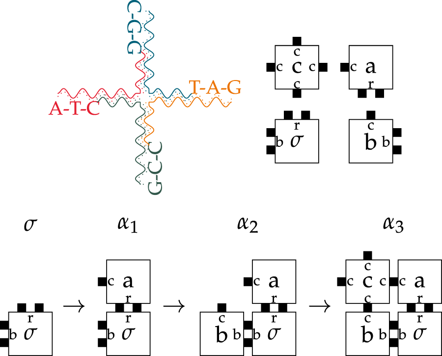
Figure 1. Example of a biological tile with four DNA-Sequences (top left) and a tileset with four independent Tiles (top right). The step-by-step assembly sequence for the tileset (Bottom). The seed tile is called $\sigma$ and the temperature is 2. $S=⟨{\alpha }_0,\dots ,{\alpha }_3⟩$ shows the three necessary steps up to the terminal Assembly.

The length of the open ends can be chosen at will and depends on the intended use case. Longer open ends result in stronger bindings, while shorter ends lead to smaller tiles with weaker binding strength. Further, the bases Cytosine and Guanine bind roughly twice as strongly as Adenine and Thymine. We model the open strand ends using arbitrary labels that represent DNA sequences, known as glues. Tiles also have a marker in the middle for visualization and are subject to environmental temperature, which affects the stability of their bindings.

The temperature is defined as the number of necessary glues for tiles to stably interact with each other to form an assembly. The binding interaction can be seen in the bottom row of Figure 1. The process starts at the bottom left with the seed-tile $\sigma$. In each simulation step, a single tile of fitting strength (number of black boxes) and label may be added to the assembly. In this case, the temperature is 2 and a stable binding requires at least two fitting glues from neighboring tiles. In steps ${\alpha }_1$ and ${\alpha }_2$, two fitting tiles with glues r and b are added. In step ${\alpha }_3$ the necessary two glues for a stable binding are provided by the two neighboring tiles a and b. At any given point in time, the growth front is the sum of positions around an assembly where new tiles could theoretically bind.

Tile assembly systems are able to perform arbitrary computations and are Turing-complete (Winfree et al., 1998). Further, the tiles themselves are small molecules that can also be used in molecular communication or even as a construction material for nanostructures. It is even possible to form fully functional DNN out of nothing but DNA, as displayed in Figure 2 (Lau et al., 2019). The system works as follows:

Figure 2

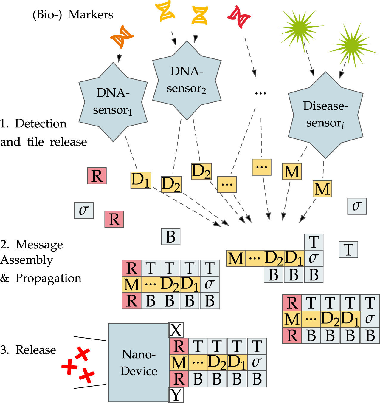
Figure 2. Identifying multiple DNA sequences or disease markers using a DNN.

DNN work based on the conditional presence of tiles. Certain nanosensors based on DNA cages, polymersomes, or liposomes can be designed to release tiles or other payload once an environmental condition is fulfilled or a biomarker/DNA sequence is present. Once released, those tiles may interact with other, already present tiles or assemblies to form message molecules that compute a decision problem while growing. Only when all necessary tiles are present may a receptor form that can in turn be detected by other nanodevices. In the case shown in the figure, a simple $n$-bit And is computed on the inputs resulting in checking for multiple conditions that have to be true at once. Once detected, the DNN may react to the findings by either reporting them via a fluorescence reaction to make them visible to the outside or directly releasing some other substance.

The primary goal of the approach presented in this paper is a more realistic simulation of the working method of such DNN.

3 Related work

We now analyze the state of the art of self-assembly simulators. Three popular tile-assembly models have mainly been used to analyze and predict DNA-based self-assembly:

1. The abstract tile-assembly model (aTAM) (Winfree et al., 1998),

2. Kinetic tile-assembly model (kTAM) (Winfree et al., 1998), and

3. The two-handed tile-assembly model (2HAM) (Demaine et al., 2016).

Each of these models focuses on a specific aspect of self-assembly, as simulating all of them at once exceeds the computational capabilities of modern computers. The aTAM is the simplest self-assembly model and a fitting individual tile is non-deterministically added to a single assembly at any simulation step. The kTAM models the process of self-assembly more realistically by introducing expected errors into the process. Instead of adding a fitting tile, a random tile is added to the assembly at any given step in time regardless of the label. The 2HAM introduces parallelism into the self-assembly process. There is no longer any dedicated seed tile and all possible assemblies that may form from a given set of tiles and assemblies are stored in each simulation step. While the 2HAM is generally computationally infeasible, it is nonetheless of great importance for simulating the often small, finite assemblies that are relevant for DNA-based nanonetworks. The Kinetic two-handed Tile Assembly Model (kTHAM), introduced in Section 5, combines aspects of both the kTAM and the 2HAM into a large parallel simulation of unique assemblies that assemble according to the rules of the kTAM. While the 2HAM is already extremely difficult to compute, it is nonetheless beneficial for the small tasks that nanonetworks likely face.

There are several existing simulators that implement some of the aforementioned models. A well-known simulator is Xgrow by Eric Winfree (Winfree et al., 2013). This simulator is written in C and is available for Windows. Xgrow is mainly used to investigate faulty assemblies. Xgrow can simulate different assemblies in parallel and implements the aTAM and kTAM models. This simulator is many times faster than other simulators such as ISU TAS, since numerous alternatives are precalculated in Xgrow. However, due to these optimizations, only constant-sized assemblies can be simulated. Since the ISU TAS is more modern and usually better accessible, the Xgrow software is rarely used, and further development is discontinued.

ISU TAS (Patitz, 2018) is an open-source simulator developed in C++ and is available for Windows, Linux and Mac OS X. The ISU TAS offers the possibility to simulate the aTAM, the kTAM and the 2HAM. However, as overall software development frameworks improved and expectations changed, several problems emerged with the ISU TAS. First, it does not use a standardized format to store its tiles. If a researcher tries to use a tileset in another software, an interpreter for this format must be written. Further, the ISU TAS is no longer in development and has been replaced by the PyTAS. As a result, the ISU TAS will not be executable in the long run due to updates in C++ or the operating systems.

The PyTAS (Patitz, 2023) is a simulator under development written in Python 3. It is only available in a beta release thus far and seems to be discontinued. The PyTAS only supports the aTAM, meaning for simulations of the kTAM or 2HAM the ISU TAS has to be used until further notice.

The WebTAS is a web app in progress. It is functional but only offers support for the simulation of the aTAM at the time of writing this paper. When and if the development of the WebTAS, as well as the PyTAS, will be finished is still unknown. Until then, they do not offer a suitable alternative for the ISU TAS.

For these and other reasons, we decided to write the NetTAS software basis from scratch to allow for the simulation of DNN, as well as the long-term support and ease of use in a web browser with multiple LATEX-related convenience features.

4 The NetTAS simulator

This section introduces the NetTAS simulator and its most important components. We start with the underlying simulation model and present the key data structures that enable the efficient simulation of self-assembly systems in web browsers like Chrome or Firefox. We also present the major components of the Software and their interaction as well as the user interface.

4.1 The NetTAS model

The NetTAS simulator was implemented using Angular, as it meets industry standards and offers a user-friendly development environment. Angular natively supports both the Model-View-ViewModel (MVVM) and Model-View-Controller (MVC) architectural patterns. NetTAS was developed following the MVVM structure, where the view is connected to the model bidirectionally through the view model. This allows changes in the model to be immediately reflected in the view, and vice versa.

The model was implemented in an object-oriented manner, strictly adhering to Winfree’s definitions for aTAM and kTAM (Winfree et al., 1998). A Tile consists of four Glue elements and one label. The label is represented directly as text. Each Glue is defined as a tuple $g=\{l,s\}$, where $l$ is the label and $s$ is the strength of the glue.

New tilesets can be created directly within NetTAS. Alternatively, users can import existing sets from JSON or ISU TAS files. Once a tileset has been created, it can be saved in JSON format for future reuse.

In addition to Glue and Tile, there are two other fundamental data types: Direction and Position. Direction is an enumeration that defines the four cardinal directions–Top, Right, Bottom, and Left–as well as the Self direction. This enumeration facilitates directional iteration and helps avoid code duplication.

Position stores the $x$ and $y$ coordinates used to define specific locations within the assembly.

The TileAssembly class utilizes the created Tiles to execute simulations. Additionally, it maintains the current growthfront. For this purpose, the changes to the growth front are checked with every assembly or breaking process. In the worst case, this means four checks per process. Checking at each process where another assembly can be connected would always require checks on the size of the assembly. Since new tiles can only attach to this growth front in subsequent steps, tracking it enables efficient simulation updates. Additionally, TileAssembly keeps track of the overall size of the assembly, allowing this information to be accessed without iterating through all individual AssemblyNodes. This improves the efficiency of comparing two assemblies for structural equivalence.

In the initial implementation attempts, the Tiles were stored in a two-dimensional array. However, since assemblies can grow in all four directions, the array had to be continuously resized, which was time-consuming and resulted in the creation of many unnecessary Tiles.

A more critical limitation of arrays is that they do not support negative indexing. This means that if the assembly expands in the negative x or y direction, every access to the array had to be recalculated whenever the array was resized. Managing this overhead in an acceptable runtime proved to be non-trivial, prompting the search for an alternative data structure.

The chosen alternative was a hash map. Hash maps offer fast access times and only require the creation of Tiles that are actually needed. However, TypeScript does not natively support hash maps with compound keys. To address this limitation, a custom data structure called PositionMap was implemented which creates a bidirectional link between a Tile and a Position.

In addition to storing Tiles in the PositionMap, each Tile also contains its own Position. This is necessary to determine the location of a given Tile during access, enabling further computations based on its position. For example, each Tile can directly check how strong its current glue strength is.

The individual simulators for aTAM, kTAM and 2HAM utilize TileAssembly instances in different ways and their simulation follow the definitions of Winfree (Winfree et al., 1998). Both the aTAM and kTAM simulators require only a single TileAssembly, on which they place a seed tile at a designated rootNode. From this seed tile, the assembly is grown. In each time step, Positions are randomly selected from the growthfront until either a suitable tile is found or all elements in the growthfront have been considered. For the selected element, tiles from the tileset are tested sequentially to determine whether one can be placed at that position in a $\tau$-stable manner. If no suitable tile is found, the algorithm proceeds to the next element in the growthfront. Once a valid tile is identified, it is placed, and the step is completed. Due to the random selection of elements from the growthfront, the aTAM process is inherently non-deterministic.

The kTAM operates differently in this regard. When adding a tile, a random Position is selected, and a randomly chosen Tile is placed at that position. Removing a tile presents a greater challenge for the implementation. The basic process involves first removing the Tile, then undoing all changes caused by this Tile. This includes the re-evaluating and recalculating the overall bond strength of the neighboring tiles. However, it is possible that other Tiles are attached to the removed Tile, which may no longer be connected to the assembly after its removal. Thus, whenever a Tile is removed, it is necessary to check which Tiles are still connected to the assembly. This becomes particularly problematic for very large assemblies, as such checks can significantly degrade runtime performance. To address this, each AssemblyNode stores the Tiles that were added to the assembly after it, referred to as its Children. As a result, when a Tile is removed, only these Children need to be checked to ensure they are still connected to the assembly. This reduces the check from all Tiles in the assembly to just the Children, which should typically be much smaller, since Tiles generally fall off before any new Tiles can attach to them.

In contrast, the 2HAM simulator operates on multiple aTAMAssembly instances, attempting to combine them into new aTAMAssembly structures. The merging of two assemblies is done iteratively. Starting from the merge point, the second assembly is iterated through. In each iteration step, the current Tile is inserted into the first assembly. This approach takes longer than directly merging the assemblies at the merge point, but it ensures that all dependencies, such as the growthfront or the neighboring relationships, are correctly set. A direct merge would require iterating through the entire assembly to achieve the same result. To improve runtime, not every assembly is merged with every other assembly in each step. Instead, only the assemblies added in the last step are attempted to be merged with all other assemblies. Furthermore, when creating new assemblies, only truly new assemblies are stored. This means that each new assembly is checked to see if it already exists. In general, this check can be significantly optimized by keeping track of the overall size of an assembly, to reduce the number of possible candidates. The kTHAM uses a combination of 2HAM and kTAM implementation for simulation, which is described in more detail in Section 5.

4.2 The user interface

The latest update of the NetTAS introduces several changes on the layout and graphical user interface. The goal was to increase the usability and make it more expandable for the introduction of future simulation modes. A key aspect of this design is the restructuring of the tileset page where the tile is placed in the middle (see Figure 3). It reduces cognitive load and is minimizing navigation effort (Nielsen, 1994). By placing core elements in an accessible area, the user can interact more intuitively, aligning with established principles of user-centered design (Norman, 2013).

Figure 3

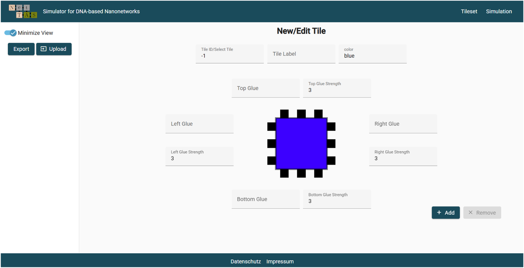
Figure 3. The new tileset view and editor.

Furthermore, by adding new tabs for the navigation to the different simulation models, switching between them is simple and does not involve switching pages anymore. This leads to a more efficient workflow when working on more complex scenarios and emphasizes the benefits of multi-tabbed interfaces for task efficiency (Cockburn et al., 2003). In addition, the code structure is more optimized for future features and maintainability. These enhancements contribute to an improved user experience and are likely to be advantageous in the future.

5 The kinetic two-handed tile assembly model

For a realistic simulation of self-assembly processes within nanonetworks, a more specialized simulation model is necessary. In this section, we define the new Kinetic two-handed Tile Assembly Model (kTHAM). It is based on the 2HAM and extends the model using properties of the kTAM. The simulation focuses on the assembly processes and does not model the nanodevices mentioned in Figure 2. For more details on the underlying implementation and a web-based application, the interested reader is encouraged to see (Kaussow, 2022b; Kaussow, 2022a).

5.1 The kTHAM model

In the kTHAM, a finite number of tiles is located in a common medium. Unlike aTAM and kTAM, the restriction to one seed tile is removed. Instead, all tiles and assemblies can freely interact with each other and form bindings, as long as a combination is somewhat realistically possible. This behavior is based on a combination of both the kTAM and the 2HAM.

As the 2HAM has a very high runtime already, we allow for a simulation speed-up by specifying a minimum number of glues that must match, the minimum binding temperature ${\tau }_{\text{min}}$. This simplification is necessary to keep the complexity of the simulation in terms of runtime and memory requirements as low as possible while still allowing for realism if needed. By adjusting parameters, the simulation can be tuned in one or the other way.

Further, at any point in time, individual tiles may disassociate from each assembly and even entire assemblies can break into two pieces. If an assembly is created from different original assemblies, the assemblies into which it breaks are selected at random. This selection is modified by the resulting bonds–an assembly is more likely to break at an unstable position.

The following parameters specify the kTHAM:

• A tileset $T$,

• the initial number of tiles of each type expressed as the state $Z_0$,

• the forward Rate $k_f$,

• the monomer concentration $G_{\text{mc}}$,

• the cost of breaking a single bond $G_{\text{se}}$,

• and the minimum binding temperature ${\tau }_{\text{min}}$.

An example of the state $Z_i$ of a kTHAM instance can be seen in Figure 4. Multiple tiles and assemblies coexist and may influence each other, resulting in a large space of possible structures. For engineering/networking purposes, a fixed number of tiles is more beneficial than the assumption of infinitely many.

Figure 4

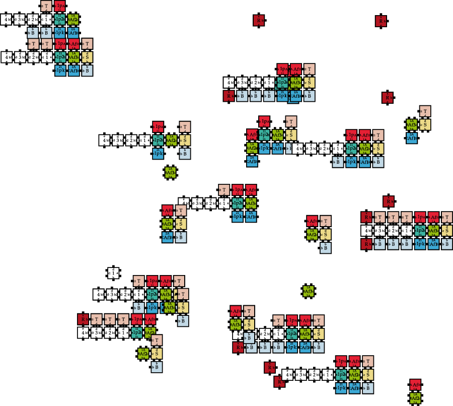
Figure 4. An overview of existing message molecules or intermediate assemblies in the kTHAM given 100 tiles of each type and parameters $G_{mc}=17$, $G_{se}=10.4$, and ${\tau }_{\text{min}}$.

A state in the kTHAM contains the information how often each tile or assembly occurs in the simulated area. Each assembly has the same probability of being selected to interact with a random assembly in each simulation step. Thus, the probability of selecting an assembly only changes based on its frequency.

In the most general case, the simulation itself does not terminate unless manually stopped. However, it is possible to specify a desired assembly from a prior simulation run that may serve as a “stopping point” for future runs in a loop.

5.2 Real-time in the kTHAM

One of the most important results of DNN simulations is the required duration in real time. This section explains how real time is modeled in the kTHAM and how different parameters influence the simulation. As the kTHAM is implemented in parallel to achieve more timely results, this posed an additional challenge.

The estimation of the real-time is based on the work of Winfree (Winfree et al., 1998). The time $t$ is computed by summing up the time that passes between the states $Z_i$ and $Z_{i+1}$ that mark successive steps of a kTHAM simulation. The time can be described as the reciprocal of the reaction rates $r_f+r_b$. These rates can be computed using the parameters $k_f$, $G_{\text{mc}}$, $G_{\text{se}}$ of the kTAM as well as the initial amount of tiles per tile type.

The required time can be stated as follows: $t(k)={\sum }_{i=1}^k\frac{1}{{r_f}_i+{r_r}_i}$.

r_f models all possible reactions between available assemblies and tiles $C_Z$ given ${\tau }_{\text{min}}$ within the state $Z$ and is based on Winfree: $r_f={\sum }_{i\in C_Z}i\cdot 20k_f{e}^{-G_{\text{mc}}}$. ${\tau }_{\text{min}}$ influences the accuracy of the simulation and can be used to speed up the process in exchange for accuracy. When this parameter is set to 0, all assemblies or tiles may form an assembly even if the resulting structure is very unstable. However, this comes at the expense of simulating errors.

$r_r$ models all already computed binding reactions for assemblies in $Z$. At these points, the assemblies are most likely to break again. All of these assemblies have a binding strength $b$ greater than or equal to ${\tau }_{\text{min}}$, which is part of $A_C$ for each assembly in $C_Z$. Based on this, all possible rates for breaking bonds are summed up as: $r_r={\sum }_{i\in C_Z}(i\cdot {\sum }_{b\in A_C}20k_f{e}^{-b{G}_{\text{se}}})$.

The resulting time of the simulation will be influenced by changing the number of tiles per tile type in the initial state $Z_0$. Fewer tiles allow for a faster simulation, and changing ${\tau }_{\text{min}}$ to a higher value leads to a faster simulation as well.

For a realistic simulation, the parameters have to be chosen carefully. Not all possible values correspond to suitable values of wet lab experiments. Small changes in the environmental parameters can lead to large changes in the resulting time. Both the relation between the values as well as the absolute values are important. The default values of the simulation correspond to the prior simulations of wet lab experiments in (Rothemund et al., 2004) but may be adjusted if necessary.

6 Evaluation

This section evaluates the kTHAM model of the NetTAS simulator. We first compare the complexity of the model with the 2HAM. After that, we demonstrate how the simulation results compare to the 2HAM and the kTAM and finally compare the real-time behavior with Winfree’s equations.

6.1 kTHAM runtime analysis

Technically, self-assembly systems are computational models and as such, the runtime of the simulation depends on the tileset, which is akin to a program with regular computers. As such, every tileset has to be considered individually as well. For especially bad tilesets, the 2HAM and kTHAM are computationally infeasible and can achieve complexities of up to $\mathcal{O}(n^n)$.

This can be easily seen by using just two tiles with identical glues that match the temperature threshold and allow for stable possible bindings in all directions. The resulting simulation does not terminate and the number of assemblies that have to be considered at each simulation step can be compared with the faculty function. Yet, the 2HAM and kTHAM are still useful for the small and finite assemblies that suffice for simulating often resource-constrained DNN (Akyildiz et al., 2008).

We still try to give an estimate of the expected complexity of the kTHAM. The kTHAM can be separated into two parts: the start and the execution of simulation steps. The start of the kTHAM is equivalent to the start of the 2HAM, since a separate assembly must be considered for each existing tile/assembly.

A step of the kTHAM is divided into determining whether an assembly breaks down or whether two assemblies or tiles combine. The runtime is the same as with the kTAM and is part of $O(n)$, with $n$ being the size of the assembly. Secondly, a step consists of either combining or breaking assemblies. The breaking can be computed in $O(1)$ as we only select from the prior components and assembly has been created from.

The combining of two assemblies is realized in $O(1)$ if and only if this combination has been computed and saved already. Initially, the assembly takes $O(Wm)$ where $W$ is the size of the growth front and $m$ is the size of the second assembly. Each point on the growth front must be considered to see if it matches each tile from the second assembly. This means that a single kTHAM step requires $O(Wm)$ steps. However, the total number of required steps cannot be known in advance due to the halting problem and the non-deterministic/random nature of the kTAM and therefore also the kTHAM.

6.2 Proof of concept of the kTHAM using a 4-bit-AND

We now demonstrate the correctness of the kTHAM by showing that it is a combination of the kTAM and 2HAM models already validated by Winfree and others. In essence, the kTHAM simulation steps are computed exactly as in the kTAM only that possibly hundreds of assemblies may coexist at the same time and interact with each other. The rules of assembly-interaction are described by the 2HAM and the remaining assembly behavior is guided by the rules of the 2HAM. As such, most assemblies formed by the interaction of two sub-assemblies may also be reached by the kTAM alone. The only exception are assemblies where the binding is based on multiple glues from different parts of the assembly. In such cases, the simulation behaves exactly like the 2HAM with the exception that assemblies created in such a way may also break apart again. However, due to the computational complexity, assemblies may not break apart arbitrarily but only either one tile at a time or at the prior points of interaction between two assemblies.

We further numerically demonstrate the intended behavior by simulating an example molecule in both kTAM and 2HAM and demonstrate that the kTHAM indeed behaves like a combination of both. The chosen molecule can be seen in Figure 5 and includes the tiles of the 4-bit-And molecule (Lau et al., 2019). The molecule only fully assembles in the presence of the four tiles 1–4. Once those are present, a receptor may attach to the assembly and finalize the message molecule.

Figure 5

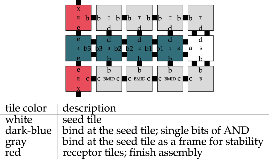
Figure 5. The output assembly of the NetTAS after simulating the tileset from Figure 6 in the different modules of the NetTAS.

For the comparison simulation in the kTAM of the ISU TAS, we used the parameters $G_{se}=10.4$ and $G_{mc}=17.0$. Here $G_{\text{mc}}$ describes the monomer concentration present and $G_{\text{se}}$ the cost of breaking a bond.

Next, the tiles from Figure 6 have also been simulated in the 2HAM of NetTAS. Both the 4-bit-And molecule and a possible message receptor at a nanodevice assemble from the same tileset. We can only model the receptor in the 2HAM, since there is no seed tile specified and many assemblies or tiles assembled in parallel.

Figure 6

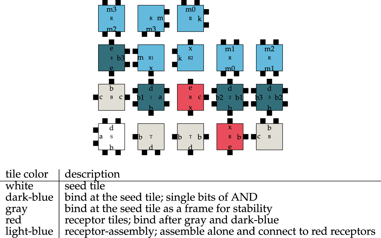
Figure 6. Tileset of a 4 Bit-And molecule in the NetTAS.

Due to the design of the two assemblies, there can only be an interaction between them when they are both completely assembled. There are countless possibilities to create smaller intermediate assemblies. However, the assembly consisting of the 4-bit-And molecule and the receptor is unique.

Both the number of possible assemblies and the resulting assembly correspond exactly to (Lau et al., 2019) where the ISU TAS was used. In the aTAM and 2HAM, the NetTAS can reproduce the results of the ISU TAS for the 4-bit-And molecule.

However, the kTAM simulation results of the 4-bit-And differed greatly from those of the ISU TAS. The reason for this is the probability computation of the add-event from Winfree’s dissertation (Winfree et al., 1998). This is defined as $p_{\text{on}}=n{k}_f{e}^{-G_{\text{mc}}}$ and the NetTAS follows exactly this definition (Winfree et al., 1998).

In the ISU TAS, the probability computation is implemented by the usage of an attachmentEvent and an detachmentEvent. Here, the attachmentEvent corresponds to the add-event from Winfree’s dissertation (Winfree et al., 1998) and the detachmentEvent corresponds to the detach-event. The ISU TAS does not implement the constant $k_f$, because it is contained in the add-event and detach-event and may be omitted. In the ISU TAS the value total is added. This changes the computation of an attachmentEvent. In the ISU TAS, the total number of tiles in a given medium grows with the number of specified tile types. In the NetTAS, we fixed the overall concentration of tiles. When more tile types are added, their overall concentration is lowered. In the kTHAM, we simply specify the total amount of tiles of each type and do not assume an infinite supply of a given concentration. While the ISU TAS correctly simulates the first few seconds of a self-assembly process, the NetTAS aims at simulating the interaction of a less well-mixed solution of possibly minutes or hours.

This means that in the ISU TAS kTAM, an assembly with many tiles can also form at lower temperatures, or that assemblies can form more quickly. A simple way to check this change is to duplicate tiles in a tileset. To do this, the tileset from Figure 6 was modified for the 4-bit-And molecule by duplicating every tile except the seed tile. Thus, all tiles remain equally likely but are present more often in the tileset.

With the values $G_{se}=10$ and $G_{mc}=19.8$, the ISU TAS needs over 10,000 binding reactions on average to complete the assembly. If the tileset is increased tenfold, the ISU TAS needs only 3,000 binding reactions to complete the assembly. This leads to differences in the number of binding reactions between the NetTAS and ISU TAS (Winfree et al., 1998). The ISU TAS interpretation is neither better nor worse than the NetTAS interpretation. For DNN, it is just better to fix the overall concentration. Yet, those numbers can be adjusted as wised in the kTHAM.

Overall, the resulting assemblies in the kTAM function of the NetTAS and the ISU TAS are identical except for the differences in the required simulation steps. Further, the resulting intermediate assemblies in the kTHAM are all part of the 2HAM computation as we use the same underlying function for the computation minus possible errors that may occur. As such, the kTHAM performs exactly as expected and provides a combination of both kTAM and 2HAM.

6.3 Real time evaluation

Next to demonstrating the correctness of the assembly, it is also necessary to illustrate that the real-time measured by the NetTAS somewhat correctly reflects the timing of wet lab experiments. In his PhD thesis, Winfree (Winfree, 1998) shows six stages with different assembly sizes and the corresponding assembly durations. Two of these stages are shown in Figures 7a,b. These are used as a basis for comparison the real-time presented in this paper.

Figure 7

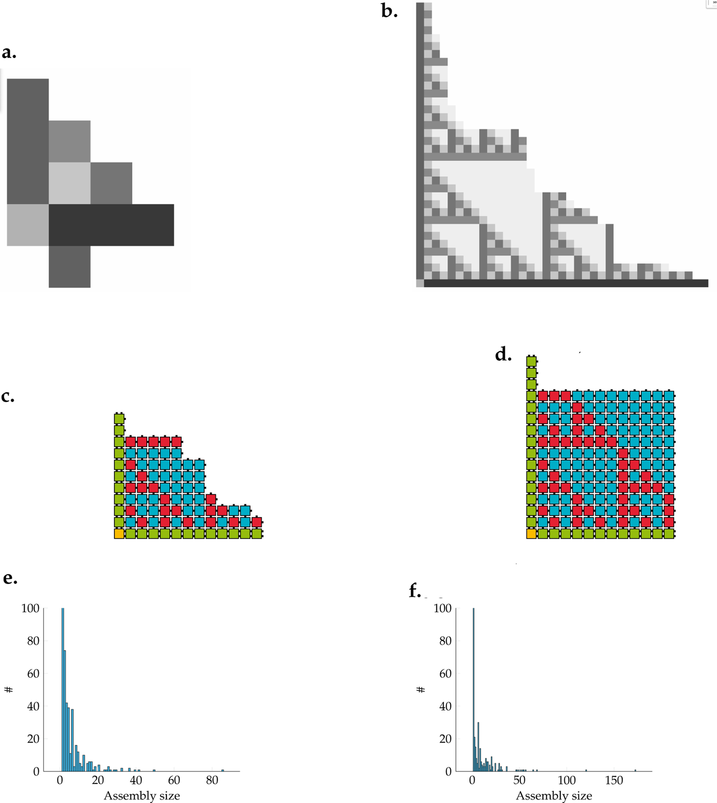
Figure 7. Comparison of the real-time between NetTAS and Winfree by simulation of the sierpinski triangle. (a) Winfree's simulation after 9s. (Winfree et al., 1998). (b) Winfree's simulation after 63s. (Winfree et al., 1998). (c) Biggest NetTAS assembly after 9s. (d) Biggest NetTAS assembly after 63s. (e) Histogram of size distributions after 9s in the kTHAM. (f) Histogram of size distributions after 63s in the kTHAM.

Winfree chose the parameters $G_{\text{se}}=8$ and $\mathcal{T}=1.95$ (Winfree, 1998) for his wet-lab experiments while (Rothemund et al., 2004) successfully used $G_{\text{se}}=10.4$ and $G_{\text{mc}}=17$. Those values correspond to 32.7 and 41.8 °C respectively. The temperature of the system can be chosen according to the desired assembly speed and the number of errors that may be tolerated (Winfree, 1998). If the temperature is chosen precisely, the number of errors may converge to zero while the speed of the assembly approaches infinity. Winfree further chose $r_f=2/\text{s}$ which corresponds to a forward rate of $k_f=600.000\frac{M}{s}$². We chose ${\tau }_{\text{min}}=2$ as a default as this allows for a feasible simulation speed.

The NetTAS simulation uses the following parameters:

• A forward Rate $k_f=600.000$,

• $G_{\text{mc}}=\mathrm{15,6}$,

• $G_{\text{se}}=8$,

• 500 tiles of each type,

• a minimal binding temperature ${\tau }_{\text{min}}=2$.

In Figures 7c,d the two stages after 9 and 63 s are shown. Below, in Figures 7e,f, the number of assemblies by size for the corresponding time points is shown as a histogram. The x-axes are limited to 100 and therefore do not show all assemblies of size one. It can be seen that there are many small assemblies.

The computed real-time of the simulation can be compared with the results of Winfree, since he has already carried out a similar simulation with his implementation of the kTAM. It should be noted that the simulations were carried out using different models. Winfree uses the kTAM, while in this work the kTHAM is used. The result of a single simulation is therefore not a single assembly, as with Winfree, but a (multi)set of assemblies. After a 9-s simulation, it can be seen that the largest assembly from the NetTAS kTHAM simulation (Figure 7c) with 85 tiles is significantly larger than the eleven tiles in Winfree’s representation. Due to the high number of assemblies simulated at the same time, the largest assembly is likely always an “outlier” and much bigger in a short time compared to the average.

Most tiles that already have at least one connection to other tiles form assemblies with a size of two to twelve tiles. This conforms to Winfree’s example, which consists of eleven tiles. After 63 s, Winfree’s assembly consists of 490 tiles, while the largest assembly from the NetTAS simulation consists of only 172 tiles. At this point, there is a clear difference between the two simulations. This difference can be explained by the different models, since with kTHAM, the edge tiles are no longer present individually after a certain point and the largest assembly cannot grow any further. None of the initial 500 tiles are available anymore while the ISU TAS and other models still assume an infinite supply of tiles of each type at any given time.

This effect could be mitigated by increasing the initial supply of tiles of chosen tiles. Yet, an additional increase in tiles quickly results in infeasible simulation times as the kTHAM is already quite slow due to the potentially very large number of assemblies simulated at the same time. This is the biggest theoretical disadvantage of kTHAM. Luckily, most proposed medical applications are relatively simple in terms of their computational complexity and the expected computational power of individual nanodevices is so low, that the kTHAM should be able to simulate most realistic scenarios without difficulty. Lau et al. (2017); Akyildiz et al. (2008).

The test further shows that the real-time is not computed entirely accurate with the simplification parameter ${\tau }_{\text{min}}=0$ – however, it is still pretty close. This is due to the optimization that has been carried out, which parallelizes the computation of the reactions. To avoid this problem and still perform a simulation with ${\tau }_{\text{min}}=0$, it is recommended to deactivate parallelization for the simulation with ${\tau }_{\text{min}}=0$. The resulting longer computation times must be accepted in this case for the correct calculation of the real-time and, if possible, reduced again by optimizing the implementation. After this change, the real-time must be validated with the corresponding parameters.

7 Summary and future work

In this paper, we presented the new NetTAS simulator with its kTHAM simulation model. The kTHAM extends the established kTAM module by introducing the parallelism of the 2HAM model. As there is no longer any dedicated seed assembly or seed tile, we can observe the interaction between all intermediate assembly products at any time and check for unwanted interactions. For the first time, this allows us to simulate simple networking scenarios holistically. Overall, this allows for the more realistic simulation of a variety of nanonetworking scenarios based on DNA.

In addition to that, we have introduced timing features into the simulation model to accurately reflect the necessary time for assemblies to form. Especially in medical scenarios or nanonetworks inside the human body, this information is crucial to assess the feasibility of a proposed approach. To evaluate the correctness, we have aligned our method with prior results from Erik Winfree’s formulas for the kTAM that we have modified for the parallel setting.

To demonstrate the correctness of the kTHAM model overall, we have first shown that the aTAM, kTAM and 2HAM modules of the NetTAS produce the same results as the ISU TAS simulator in most cases. The kTHAM itself uses the same methods to simulate kTAM in parallel. We further demonstrated that the kTHAM’s result matches the findings of the 2HAM when it comes to assembly interactions and the kTAM when it comes to erroneous DNA bindings. The NetTAS is a suitable, modular and extendable basis for many novel features and some of them are already in development. The source code is available in a Git repository (Kaussow, 2022b) and the simulator is also available online (Kaussow, 2022a).

While the kTHAM is a major improvement over existing models for networking applications, other modules were mainly designed for simulating DNA-based computations. This is especially true for in-body nanonetworks (Lau et al., 2019; Akyildiz et al., 2008). It might be possible to model the human circulatory system using a Markov model to determine the concentration of all self-assembly components in distinct segments of the human body. As such, it might be possible to accurately simulate self-assembly processes in the entire human body and not just small segments.

Another possible improvement would be the introduction of a chance to start the simulation with assemblies instead of just tiles to better simulate possible real world conditions. This basic functionality could also serve as a basis for the introduction of new assemblies once specific simulation conditions have been met. In doing so, the NetTAS would be able to simulate an entire array of more complex network protocols that rely on the exchange of message molecules for, e.g., synchronization purposes.

Data availability statement

Publicly available datasets were analyzed in this study. This data can be found here: https://git.itm.uni-luebeck.de/kaussow/nettas.

Author contributions

MK: Validation, Supervision, Writing – review and editing, Software, Visualization, Writing – original draft. RP: Software, Writing – original draft. SS: Writing – review and editing, Software, Writing – original draft. CH: Writing – review and editing, Software, Writing – original draft. SF: Supervision, Writing – review and editing. FL: Writing – original draft, Supervision, Software, Writing – review and editing, Project administration.

Funding

The author(s) declared that financial support was received for this work and/or its publication. This work has been supported in part by the German Research Foundation (DFG): Project 419981515, NaBoCom II and the BMBF-financed Project 16KIS1991, IoBNT.

Conflict of interest

The author(s) declared that this work was conducted in the absence of any commercial or financial relationships that could be construed as a potential conflict of interest.

Generative AI statement

The author(s) declared that generative AI was not used in the creation of this manuscript.

Any alternative text (alt text) provided alongside figures in this article has been generated by Frontiers with the support of artificial intelligence and reasonable efforts have been made to ensure accuracy, including review by the authors wherever possible. If you identify any issues, please contact us.

Publisher’s note

All claims expressed in this article are solely those of the authors and do not necessarily represent those of their affiliated organizations, or those of the publisher, the editors and the reviewers. Any product that may be evaluated in this article, or claim that may be made by its manufacturer, is not guaranteed or endorsed by the publisher.

Footnotes

¹https://nettas.itm.uni-luebeck.de

²$r_f(t)=20k_f{e}^{-G_{\text{mc}}}=20\cdot 600.000e^{-\mathrm{15,6}}=\mathrm{2,015}$.

References

Akyildiz, I. F., Brunetti, F., and Blázquez, C. (2008). Nanonetworks: a new communication paradigm. Comput. Netw. 52, 2260–2279. doi:10.1016/j.comnet.2008.04.001

CrossRef Full Text | Google Scholar

Cockburn, A., Gutwin, C., and Greenberg, S. (2003). “A predictive model of menu performance,” in Proceedings of the SIGCHI conference on human factors in computing systems (New York, NY, USA: ACM), 431–438. doi:10.1145/642611.642682

CrossRef Full Text | Google Scholar

Demaine, E. D., Patitz, M. J., Rogers, T. A., Schweller, R. T., Summers, S. M., and Woods, D. (2016). The two-handed tile assembly model is not intrinsically universal. Algorithmica 74, 812–850. doi:10.1007/s00453-015-9976-y

CrossRef Full Text | Google Scholar

Kaussow, M. (2022a). NetTAS. Available online at: https://nettas.itm.uni-luebeck.de/.

Google Scholar

Kaussow, M. (2022b). NetTAS gitlab. Available online at: https://git.itm.uni-luebeck.de/kaussow/nettas.

Google Scholar

Lau, F., Büther, F., and Gerlach, B. (2017). “Computational requirements for nano-machines: there is limited space at the bottom,” in 4th ACM international conference on nanoscale computing and communication (Washington DC, USA). ACM NanoCom’17.

Google Scholar

Lau, F.-L. A., Büther, F., Geyer, R., and Fischer, S. (2019). Computation of decision problems within messages in dna-tile-based molecular nanonetworks. Nano Commun. Netw. 21, 100245. doi:10.1016/j.nancom.2019.05.002

CrossRef Full Text | Google Scholar

Nielsen, J. (1994). Usability engineering. San Francisco, CA, USA: Morgan Kaufmann.

Google Scholar

Norman, D. A. (2013). The design of everyday things. New York, NY, USA: Basic Books. revised and expanded edn.

Google Scholar

Patitz, M. J. (2011). Simulation of self-assembly in the abstract tile assembly model with isu tas. arXiv Preprint arXiv:1101. doi:10.48550/arXiv.1101.5151

CrossRef Full Text | Google Scholar

Patitz, M. J. (2014). An introduction to tile-based self-assembly and a survey of recent results. Nat. Comput. 13, 195–224. doi:10.1007/s11047-013-9379-4

CrossRef Full Text | Google Scholar

Patitz, M. J. (2018). Isu tas. Fayetteville, AR: Patitz University of Arkansas Fayetteville.

Google Scholar

Patitz, M. J. (2023). Pytas.

Google Scholar

Paun, G., Rozenberg, G., and Salomaa, A. (2005). DNA computing: new computing paradigms. Springer Science & Business Media.

Google Scholar

Rothemund, P. W. K., Papadakis, N., and Winfree, E. (2004). Algorithmic self-assembly of dna sierpinski triangles. PLOS Biol. 2, null. doi:10.1371/journal.pbio.0020424

PubMed Abstract | CrossRef Full Text | Google Scholar

Seeman, N. C. (1982). Nucleic acid junctions and lattices. J. Theoretical Biology 99, 237–247. doi:10.1016/0022-5193(82)90002-9

PubMed Abstract | CrossRef Full Text | Google Scholar

Winfree, E. (1998). Algorithmic self-assembly of Dna. Ph.D. thesis. USA: California Institute of Technology.

Google Scholar

Winfree, E., Liu, F., Wenzler, L. A., and Seeman, N. C. (1998). Design and self-assembly of two-dimensional dna crystals. Nature 394, 539–544. doi:10.1038/28998

PubMed Abstract | CrossRef Full Text | Google Scholar

Winfree, E., Schulman, R., and Evans, C. (2013). The xgrow simulator. CA, United States: Online.

Google Scholar