A comparative study of neural network pruning strategies for industrial applications

Introduction: In recent years, Deep Learning (DL) and Artificial Neural Networks (ANNs) have transformed industrial applications by providing automation in complex tasks such as anomaly detection and predictive maintenance. However, traditional DL models often need significant computational resources, making them unsuitable for resource-constrained edge devices. This paper explores the potential of sparse ANNs to address these challenges, focusing on their application in industrial settings.

Methods: We perform an experimental comparison of pruning techniques, including the Pre-Training, In-Training, Post-Training, and SET method, applied to the VGG16 and ResNet18 architectures, and conduct a systematic analysis of pruning methodologies alongside the effects of varying sparsity levels, to analyze their efficiency in anomaly detection and object classification tasks. Key metrics such as training accuracy, inference time, and energy consumption are analyzed to assess the feasibility of deploying sparse models on edge devices.

Results and discussion: Our results demonstrate that sparse ANNs, particularly when pruned using the SET method, achieve energy savings without compromising accuracy, making them suitable for industrial applications. This work highlights the potential of sparse neural networks to boost sustainability and efficiency in industrial environments, paving the way for their large adoption in edge computing scenarios.

1 Introduction

In recent years, Deep Learning (DL) and Artificial Neural Networks (ANNs) have transformed industrial applications by automating complex and repetitive tasks. DL algorithms, paired with sensors and camera networks, can monitor industrial processes and assist in essential tasks, such as anomaly and fault detection, and predictive maintenance. By analyzing data in real-time, these systems help industries prevent failures and optimize operations.

However, classical DL models usually require huge computation and bandwidth to process massive datasets (Rane et al., 2024; Huo et al., 2021; Balaprakash et al., 2019). For example, large-scale object detection models such as You Only Look Once (YOLO) (Redmon et al., 2016) are usually trained by migrating massive image datasets like ImageNet (Deng et al., 2009) to high-performance cloud servers for computation. This results in increased delays in communication and puts a heavy burden on bandwidth and computing resources. Such an approach is particularly inefficient and resource-intensive for systems with limited computational power, such as smartphones or IoT (i.e., Internet of Things) devices, since they lack the necessary hardware capabilities to handle such demands.

However, the rapid growth of IoT has made edge devices more capable, allowing much of the data to be processed locally instead of relying on cloud resources (Kanagarla, 2024; Brennan and Lee, 2024). This shift moves the processing burden from central systems to devices at the “edge” of the network, such as sensors or small devices near the data source (Palena et al., 2024; Kolapo et al., 2024). As a result, systems become more sustainable and energy-efficient, while reducing both bandwidth usage and latency (Taha et al., 2024). This makes edge processing essential for a wide range of applications, particularly those requiring real-time performance in industrial scenarios. Besides that, certain computationally intensive tasks, especially, those involving generative adversarial networks (GANs) for generating images, videos, or any other form of visual content (Goodfellow et al., 2014; Andriulo et al., 2024; Soumyalatha and Manjunath, 2023), still lead to challenges for edge devices due to their high resource demands compared to traditional deep learning models.

Using edge technologies is not limited to running complex deep learning algorithms on smaller or lighter hardware (Witt et al., 2024; Shuvo et al., 2023; Susskind et al., 2023). It also involves investigating methods such as optimizing network architectures, compressing models, and applying pruning techniques on the different parts of the model, among others (Wang, 2023; Zou, 2024; Blalock et al., 2020; Cheng et al., 2024).

Various optimization techniques exist to fit ANNs on lightweight devices: model compression, network pruning, and sparsity (Nimmagadda, 2025; Tyche et al., 2024). Recently, sparse ANNs have gained popularity (Lasby et al., 2023; Nikdan et al., 2023) due to their ability to produce performance very similar to those obtained with fully connected networks but that usually occupy less memory, are more lightweight and thus, have faster inference times (Erhan et al., 2025; Jayasimhan and Pabitha, 2024; Atashgahi et al., 2024). Even the most straightforward methods based on random pruning can yield very encouraging results (Sun et al., 2023; Gadhikar et al., 2022; Mittal et al., 2019). In addition, the more sophisticated dynamic sparse training could lead to gains regarding training efficiency (Li and Chang, 2024; Qu et al., 2024).

Our research focuses on industrial applications by conducting an experimental comparison of sparse ANNs on a resource-constrained laptop. We examine how various pruning methods and levels of sparsity affect the performance of ANNs in detecting anomalies and faults in industrial environments or classifying objects in the same setting. While laptops are not IoT devices, the experiments conducted allow us to lay the foundations for future deployments of industrial applications at the edge. To evaluate the convenience of using these techniques in an IoT edge context, we analyze key metrics such as training accuracy, training loss, total training time, and average inference time. Additionally, we consider energy consumption from a sustainability perspective, estimating the energy required to train the models and also during the inference phase.

2 Related work

Our research focuses on using sparse ANNs for industrial applications, where efficiency and computational cost are critical factors to be considered. While industrial datasets present unique challenges, such as handling high-resolution images (e.g., MvTec3D; Section 3.3.2) or limited samples in anomaly detection tasks (e.g., VisA; Section 3.3.3), sparse models offer a solution to reduce resource requirements without compromising performance. However, before applying sparsity techniques (Section 3.1) to complex industrial datasets, it is crucial to validate their effectiveness in a controlled environment. This approach ensures that the sparsification methods are strong and generalizable before addressing the specific challenges of industrial data.

According to this need, we chose MedMNIST as a benchmark because it provides a standardized and diverse set of medical imaging tasks, making it ideal for validating our sparsity techniques. Yang et al. (2021) created this dataset, which aims to facilitate rapid prototyping and provide an easy benchmark with which comparison between medical image analysis models can be made. The authors tested various baseline methods, including ResNet variations and AutoML tools, supporting the claim that the utility of the dataset might advance research.

To validate our approach, we built upon former research that evaluated the performance of different models on MedMNIST dataset collection. Doerrich et al. (2024) presented a comprehensive study evaluating 10 different models, including VGG16 and ResNet18, on the MedMNIST collection. Their work presented a comprehensive baseline for the performance of each dataset in the MedMNIST collection. Table 1 presents the accuracy of their experiments on the BloodMNIST dataset compared to the accuracy of our experiments where we use the fully connected ANNs as well as where we employed sparsification strategies on the same methods.

Table 1

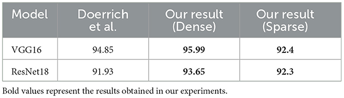
Table 1. Comparison of the best accuracy (in %) achieved by VGG16 and ResNet18 models when trained on the BloodMNIST dataset with 0% sparsity (Dense), after applying (50%) sparsity on convolution layers and (80%) sparsity on linear layers, and as reported by Doerrich et al. (2024).

In this work, our experiments achieved accuracy levels comparable to those reported in their study, validating the effectiveness of our approach( 2% increase on average). Additionally, we conducted a detailed comparison of metrics, such as sparsity levels, training time, accuracy, and inference time. These results along with a comprehensive analysis, are presented in the results section (Section 4), where we demonstrate how sparse neural networks can efficiently classify medical images while maintaining competitive performance.

The other dataset being used in this work is VisA, related to binary classification with the normal and damaged objects available in the industrial environment. As a fact, one recent work that classifies such data by making use of VisA is presented in Chen et al. (2023). They proposed an APRIL-GAN: GAN-based architecture for the participation of the VAND 2023 Challenge. Their objective was to create a model that can work with different classes, most of which require very minimal or no available normal reference images and speed adaptation.

In the zero-shot track without reference images, they extend CLIP with added layers to map image features in a common space for comparisons of text features for the effective generation of anomaly maps. For the few-shot track that has some reference images, their approach relied on memory banks for the storage of image features in order to match test images with them at runtime. Their approach achieved very good results, ranking first in the zero-shot track and fourth in the few-shot track, with a classification accuracy of 86.87%.

Nevertheless, APRIL-GAN models, have some drawbacks: they need more computational power compared to normal DL models, which limits their scalability in industrial applications. Furthermore, their architecture did not employ any sparsification methods, such as those regarding stochastic weights, that could have helped. In contrast, our method, using sparse networks, achieves comparable accuracy (86%) without the computational burden of GANs. In this research, we focus on reducing computational costs and improving efficiency by using lighter models and sparse neural networks.

Another research that shares similarities with our work in terms of dataset and using ANN solutions for industrial environment is WinCLIP, a vision-language model created by Jeong et al. (2023) for zero-shot and few-shot anomaly classification and segmentation tasks in an industrial context. In contrast to most of the strategies that have been developed and implemented with a Primary Model reliant heavily on deeply annotated datasets, WinCLIP employs the CLIP model, which has already been trained, to correlate images and text. This means that it can identify anomalies without having large amounts of annotated data. The model employs patch, window, and image multi-level features as well as prompt-engineering-based textual embeddings and is effective at classification and segmentation tasks alike.

The authors also proposed WinCLIP+, an enhancement of the previous one that utilizes additional normal image data to enhance efficiency in a few-shot learning cases. Competitive results are obtained for WinCLIP and WinCLIP+ on some datasets like MVTec-AD and the VisA, as compared to other state-of-the-art architectures in zero-shot and few-shot approaches. These results also point to the industrial anomaly detection potential of vision-language models.

Despite the advantages, WinCLIP has limitations: it depends on resource-intensive computer vision and natural language processing models, which may strain industrial resources. Additionally, the study does not explore sparse neural networks, which could further optimize performance. On the other hand, models such as VGG16 and ResNet18, which are used in their dense versions, deliver close to 86% accuracy and remain lightweight and inexpensive to implement. We further refine these models using sparsity techniques to deploy them in industrial environments more easily and maintain them more efficiently in the future. The focus of our work is therefore on more direct and performant approaches that are fitting for industrial usage and are therefore complimentary to WinCLIP.

Besides the papers that used the same datasets as our experiments, Jayasimhan and Pabitha (2024) proposed a filter pruning technique that shares similarities with our convolution-pruning approach. Their method achieves a model accuracy close to the dense version after applying a 40% average sparsity level across layers. However, their work focuses on dynamic sparsity levels, where different layers have different sparsity levels, and they do not prune the linear layers. In contrast, our work extends this approach by focusing on industrial datasets and models to simulate real-world scenarios. Additionally, we not only increase the sparsity level but also apply pruning to both convolutional and linear layers, further exploring the impact of sparsity on model performance in industrial environments.

Several surveys have explored the performance of pruning techniques across various domains, providing valuable insights into their applications and limitations such as Reed (1993), Blalock et al. (2020), and Cheng et al. (2024). Among these, Cheng et al. (2024) provides a comprehensive review of deep neural network pruning, analyzing over 300 papers to categorized the field into four key areas: (i) universal/specific, (ii) pruning timing, (iii) pruning methods, and (iv) fusion of pruning with other compression techniques. This survey includes different domains such as Computer Vision, Natural Language Processing, and Audio Signal Processing.

Extending Cheng et al. (2024)'s research, we investigate four types of pruning techniques including Pre-Training, In-Training, Post-Training, and SET method with a focus on industrial applications, an area that requires further attention. Specifically, we address gaps identified in their survey by investigating the impact of sparsification on different types of layers and focusing on industrial applications. Additionally, we compare the performance of pruning techniques in the image classification domain to provide insights appropriate for real-world needs. For instance, in our experiments, we achieve higher accuracy when pruning to obtain a 50% level of sparsity over convolutional layers, thus, presenting the effectiveness of sparse networks in addressing the industrial challenges. Additionally, we extend their findings by systematically analyzing the behavior of models when different sparsity levels are applied to different types of layers (e.g., convolutional and linear layers), a dimension not thoroughly explored in their study. By doing so, we provide deeper insights into the interplay between sparsity, layer types, and model performance, complementing the broader scope of Cheng et al. (2024)'s survey with a focused investigation tailored to industrial applications.

Although previous works have explored various aspects of industrial usage of ANNs, there are critical gaps in areas such as energy efficiency, sparsification techniques, model selection, and practical deployment that remain unaddressed. For instance, while Chen et al. (2023) and Jeong et al. (2023) achieve a comparable accuracy on their studies, they did not measure the energy efficiency of the final model, which is crucial for industrial applications where resource constraints are a major concern. Additionally, by investigating sparsification techniques we address another uncovered area of those studies. Chen et al. (2023) also rely on high-resource-needing models such as GANs, rather than leveraging efficient and widely applicable architectures e.g., VGG-16 and ResNet-18. These gaps highlight the need for more comprehensive research that addresses the practical challenges of deploying ANNs in industrial settings. Furthermore, while Cheng et al. (2024) examine the impact of varying sparsity levels across different layer types, they overlook the industrial context and utilize pruning techniques that differ from those used in our study.

To summarize, this research work tackles limited research on sparse neural networks for industrial applications by providing an experimental evaluation and comparison of four different pruning methods, namely Pre-Training, In-Training, Post-Training, and SET, applied to two models which are commonly used in industrial settings, namely VGG 16 and ResNet18. In terms of chosen datasets for carrying out this work, we chose as primary benchmark BloodMNIST, not an industrial dataset, but a well documented standardized dataset, lightweight, with minimum complexity to validate and compare our proposed approach against the usual application of dense neural networs. After a successful validation of our approach, we expand the experimental evaluation and comparison to include industrial datasets VisA, and MVTec 3D Object Classification. Monitored metrics include accuracy, training and inference time, energy usage. The results indicate that pruned neural networks achieve performance levels similar to those of their dense counterparts, while boasting reduced inference time in less powerful hardware, such as laptops running only on CPU. The results pave the way for the expansion of the analysis and study to include more complex industrial datasets and scenarios, as well as extended metric monitoring, energy efficiency and trade-off analysis while considering a variety of devices ranging from classic HPC/Cloud infrastructure to resource-constrained devices more suitable for IoT Edge deployment in an industrial setting.

3 Methodology

In this section, first in Section 3.1, we explore the sparsity definitions, the techniques we employed, and also present the mathematical formulations that define these sparsity techniques, detailing how each method was applied to the neural network models and its role in enhancing performance. Next, in Section 3.2, we describe the architectures of the models used, including specific details about their layers, configurations, and adaptations for our experiments. Then, in Section 3.3 we present each selected dataset for our experiments in detail. After that, in Section 3.4, we describe how we collect our data from the experiments to visualize them in Section 4. Finally, Section 3.5 shows our pruning scenarios and the sparsity level for each section of the models.

3.1 Sparsity

Sparsity in ANNs refers to the actions of reducing the number of active connections or weights in a network. This approach mimics biological neural systems, where only a subset of neurons and connections are active at any given time. The goal of introducing sparsity is to create more efficient models that require fewer computational resources, consume less energy, and maintain or even improve performance on specific tasks. In this research we used four different sparsity techniques including Pre-Training (Section 3.1.1), In-Training (Section 3.1.2), Post-Training (Section 3.1.3), and Sparse Evolutionary Training (Section 3.1.4).

3.1.1 Pre-training

One common pruning method employs the L1 technique (Wu et al., 2019) to remove weak connections immediately after the neural network is created but before the training process begins. By starting with a pruned network, where some of the connections according to the sparsity level have already been removed, the number of parameters to optimize is significantly reduced. This not only simplifies the optimization process but also lowers computational costs and accelerates the training phase, as the model requires fewer resources to learn effectively (Shi et al., 2024). In Section 3.1.1.1, we provide a detailed explanation of the L1 norm, including its mathematical formulation, and an example.

3.1.1.1 L1 algorithm

L1 norm is a mathematical technique used in the area of machine learning and statistics, to improve the importance of feature selection, reduce model complexity, and improve prediction accuracy. It aims at the minimization of the sum of selected variables' (e.g., the weight of the connections in our case) absolute values, hence causing “sparsity” where most variables become zero (i.e., the removed connections in our experiment). This method has a wide application in pruning techniques, signal processing, image recognition, and bioinformatics.

The L1 norm, also called the “least absolute deviation,” calculates the distance between points in a mathematical space. For a vector x = [x₁, x₂, x₃, ..., x_n], the L1 norm is defined as:

$\begin{array}{ll}||x{||}_1=\left|x_1\right|+\left|x_2\right|+...+{|x}_n|& (1)\end{array}$

This calculation sums up the absolute values of each element in the vector x. Unlike other norms, such as the L2 norm (which squares each element), the L1 norm does not exaggerate the size of larger values. This quality is what makes it suitable for creating sparse solutions, which involve many values in the vector being zero.

In machine learning, the L1 unstructured method is often applied to solve an optimization problem by minimizing a “loss function” (the difference between predicted and actual values) and adding a regularization term that uses the L1 norm. This is common in Lasso Regression, where the goal is to find coefficients for features that best predict the output while reducing the complexity of the model.

As an example, imagine we are working with three features and have the weight vector w = [w₁, w₂, w₃]. By applying the L1 unstructured method, we may end up with a solution like w = [0.5, 0, 1.2]. Here, the method set w₂ to zero, indicating that the second feature is not significant for our predictions. This outcome simplifies the model without losing much accuracy in the prediction.

3.1.2 In-training

The second pruning method uses the built-in Random technique in the PyTorch library to create the initial model. During training, at each epoch, the 20% of weakest connections (i.e., the smallest positive and largest negative weights) are swapped out for random ones that were previously removed. We used the Random technique to create the initial model. After that, we replaced the weak connections, identified by their L1 scores, with new random ones. This approach ensures that the model always retains the strongest connections. In Section 3.1.2.1, we provide a detailed explanation of this algorithm, including its formulation, and a simple example.

3.1.2.1 Random algorithm

In this random unstructured method, the features or weights of a model are randomly selected in a manner such that it simplifies the model without any regard to the importance of features. It works by zeroing out a random element and otherwise retaining elements to produce a simpler model which can sometimes, as an added advantage, help reduce overfitting. In the L1 method, sparsity is created by using an optimization process that reduces the size of certain connections in the network. This is done in a selective way, keeping the important connections while removing the less important ones. In contrast, the random unstructured method uses randomness to remove connections without any optimization or specific selection. This approach is simpler and faster than the L1 norm technique (Section 3.1.1.1) to apply but does not focus on which connections are more or less important. In other words, this randomness gives every connection, whether it is active or removed, the same chance to be included in the process. This is important because a connection that seems unimportant at the start might become very important later during training as the model learns. By treating all connections equally, the random method stays flexible and avoids removing connections that could help improve the model later.

In this method, we start with a vector x = [x₁, x₂, x₃, ..., x_n] and randomly select the indices to keep, while setting the others to zero. This can be represented as:

$\begin{array}{ll}{x}^{\prime }=\left[x_1.m_1,x_2.m_2,x_3.m_3,...,x_n.m_n\right]& (2)\end{array}$

In Equation 2, x′ is the modified vector after applying the random unstructured method, and m₁ s a binary mask (either 0 or 1) randomly assigned to each element x_i. If m_i = 0, x_i is set to zero; if m_i = 1, x_i is retained.

Assume we have a vector x = [0.7, 1.2, 0.3, 0.9, −0.4] and generate a random mask m = [1, 0, 1, 0, 1]. The result x′ after applying the random unstructured method would be x′ = [0.7, 0, 0.3, 0, −0.4] In this way, the random unstructured method does not focus on the importance of features but randomly enforces sparsity, which can sometimes be useful in preventing overfitting or reducing the computational cost. In short, the random unstructured method applies random sparsity to a vector by setting some elements to zero based on a randomly generated mask.

3.1.3 Post-training

This method is the simplest approach discussed herein. It involves pruning the network after the training process is complete. The primary advantage of this technique is that it allows us to create models with different levels of sparsity without needing to train the model multiple times. This is particularly useful because we only need the final checkpoint of the trained model to apply the pruning process.

To prune the network, we start with a fully connected model and remove the weakest connections based on their L1 scores—the same metric used in pre-training (Section 3.1.1). However, this method has some limitations. Since pruning happens after training, the model doesn't have the opportunity to optimize its weights during training to account for the removed connections. Additionally, if the model overfits during training, the pruned versions might still carry over this overfitting issue, which can affect their performance on new data.

3.1.4 SET method

The Erdös-Rényi model (Erdős and Rényi, 2022) is a fundamental mathematical framework used to generate random graphs, which consist of nodes connected by edges. This model is particularly useful for studying the structure of real-world networks, such as social or biological systems, by simulating their connectivity using probabilities. In this model, we begin with n nodes, where each possible pair of nodes is connected by an edge with a probability p. The simplicity and flexibility of this model make it an excellent tool for initializing sparse architectures in neural networks.

Building on this, the SET method, introduced by Mocanu et al. (2018), uses the Erdös-Rényi model to create an initial sparse network. Unlike the Random and L1 techniques, which follow different sparsification approaches, SET employs this probabilistic model to define the initial connections between neurons. By using the Erdös-Rényi model, SET generates a sparse network with a controlled level of connectivity based on the probability p.

During training, the SET method incorporates the In-Training Method to optimize the network parameters. It dynamically adjusts the network by replacing the 20% of smallest positive and largest negative weights (i.e., weaker connections) with connections that were pruned earlier. This process ensures that the model always builds up the most important connections while maintaining sparsity. By the end of training, the network evolves into a strong structure with highly optimized connections, effectively balancing efficiency and performance.

Having this sparsity technique, along with the In-Training approach, allows us to investigate the roles of different initialization methods, which is the only difference between these two pruning approaches. Specifically, we use the standard random model exclusively for the In-Training approaches, while the Erdös-Rényi model is utilized solely for the SET method. This comparison helps us evaluate how these initialization strategies impact the network's performance and training dynamics in their respective contexts. Algorithm 1 provides the pseudocode for the implementation of the In-Training and SET methods in our experiments.

Algorithm 1

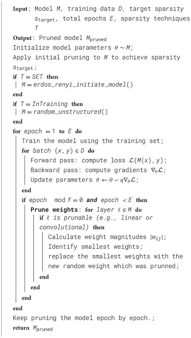
Algorithm 1. Pruning the model during the training (SET and In-Training).

3.2 Models

In this section, we will explore different model architectures that are central to our research. We provide a detailed overview of their design and functionality, explaining why they are important to our work. Two of these models - which are VGG-Net Architecture (Section 3.2.1) and ResNet Architecture (Section 3.2.2)—are directly used in our experiments as base architectures (i.e., VGG16 and ResNet18), forming the foundation of our approach. Besides that, Figure 1 provides a comparative visualization of the architectural structures of both models, highlighting their key main parts and the position of each layer type. Additionally, we discuss Generative Adversarial Networks (GANs) (Section 3.2.3), which are not directly used in our experiments but are included because they play a key role in similar research (Chen et al., 2023). By understanding GANs, we gain better insight into how related studies approach the problem. Together, these models help us build a clear picture of the methods and ideas driving our experiments.

Figure 1

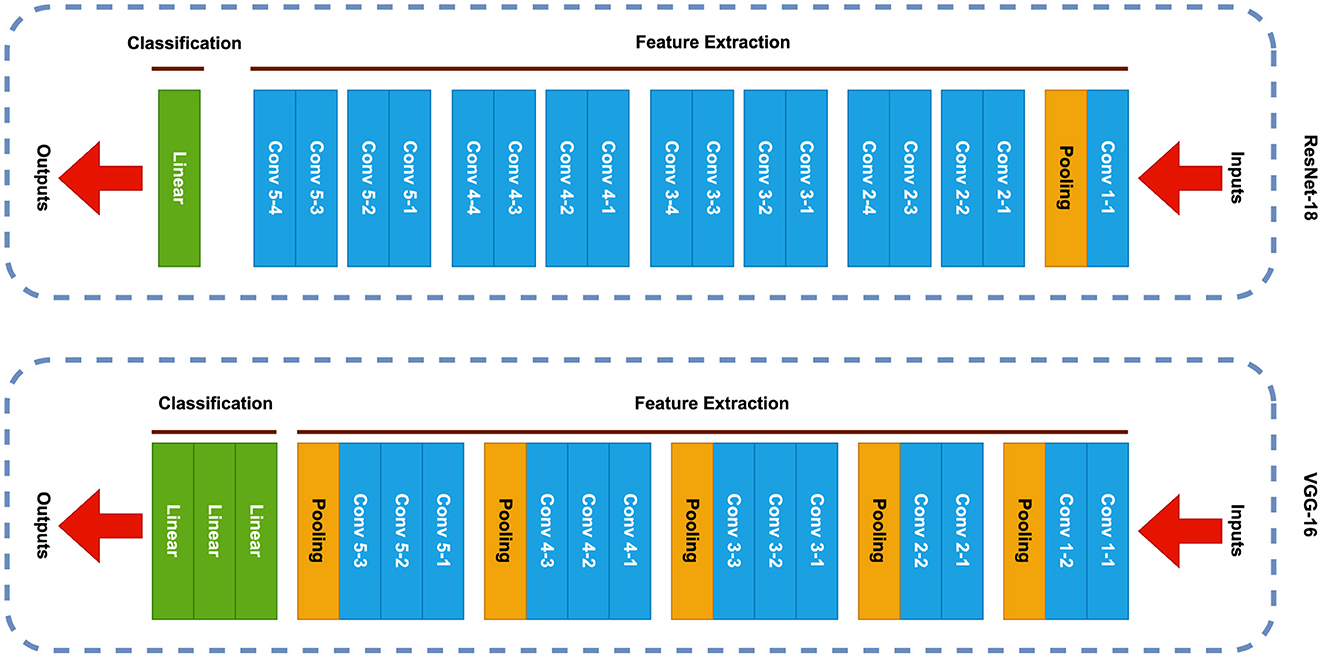
Figure 1. A simplified illustration to compare VGG16 and ResNet18 architectures at a glance.

3.2.1 VGG-Net architecture

The Visual Geometry Group (VGG) (Simonyan and Zisserman, 2014) architecture, represents a standard deep Convolutional Neural Network (CNN) design characterized by its depth, with variations such as VGG-16 and VGG-19 featuring 16 and 19 convolutional layers, respectively. This deep neural network has been instrumental in advancing object identification models. Due to its innovative design and robust capabilities, VGG continues to be one of the most widely adopted architectures in the field of image recognition (Apostolopoulos and Tzani, 2022; Hossain et al., 2019). Both these VGG architectures (i.e., VGG-16 and VGG-19) are common architectures, but for the industrial environment, efficiency is an important factor. While both models are effective, VGG-16 has approximately 138 million parameters, compared to VGG-19's 143 million. This smaller size makes VGG-16 more computationally efficient and needs fewer resources for training and deployment. In industrial settings, where resource limitations and semi-real-time processing are often priorities, VGG-16 strikes a better balance between performance and practicality. This is why we selected VGG-16 as the base architecture for our experiments.

3.2.2 ResNet architecture

The main novelty of the Residual Network (ResNet) (He et al., 2016) architecture consists of residual blocks that were introduced as a remedy for the vanishing gradients problem for very deep networks. Using skip connections, or residual connections, gradients can easily flow during backpropagation and thus allow for the training of networks with many layers, way more than was possible before like AlexNet (Krizhevsky, 2014) with 8 layers, or VGG with 16 or 19 layers. In fact, this ability to grow “very deep,” with hundreds of layers, while remaining trainable and effective, is what made ResNet a landmark in deep learning.

ResNet is one of the most widely used architectures in industrial applications due to its balance of performance (Duan et al., 2021; Xu et al., 2023; Gao et al., 2022; Lee et al., 2020). There are several versions of the ResNet architecture, including ResNet-18, ResNet-34, ResNet-50, and ResNet-101, each with different depths and complexities. The ResNet-18 and ResNet-34 represent shallow and more efficient variants, making them a suitable selection for less complicated scenarios or resource-constrained environments like industrial settings. While ResNet-50 and ResNet-101 are deeper and more powerful, they will give better results (Khan et al., 2017) on challenging tasks with larger datasets such as COCO (Lin et al., 2014); their higher complexity also means that they require many more resources than shallower models, reducing their practicality in low-resource settings, such as certain industrial applications where efficiency is very crucial. According to these facts, we select ResNet-18 for our experiment to not only have the performance of this architecture but also keep the model resource efficient.

3.2.3 Generative adversarial networks

Generative Adversarial Networks (GANs) work by training two models at the same time: a generator (G) and a discriminator (D). The generator creates new data, like images, that look similar to real data, while the discriminator tries to tell the difference between real data and the fake data created by the generator. The goal of the generator is to make the discriminator think that the fake data is real. This creates a competition between the two models, like a game, where the generator tries to get better at making fake data, and the discriminator tries to get better at spotting it. As both models improve, the generator creates more realistic data, and the discriminator becomes more accurate. This process can be trained using backpropagation, a common technique in machine learning. GANs are powerful because they can generate high-quality data without needing complex processes, like Markov chains, during training.

3.3 Dataset

In this section, we describe the datasets used in our study. Each dataset is introduced separately. The following subsections provide details on the individual datasets namely MedMNIST (Section 3.3.1), MVTec 3D Object Classification (Section 3.3.2), and VisA (Section 3.3.3). Figure 2 provides an overview of data frequency, showing how datasets are split into training, testing, and validation sets.

Figure 2

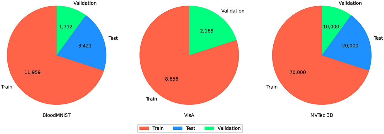
Figure 2. The pie charts illustrate the distribution of data into training, testing, and validation sets for three datasets. The color coding is fixed among datasets: Red for training, Blue for testing, and Green for validation.

For the BloodMNIST and MVTec3D datasets, the training phase uses 70% of the data, while the remaining 30% is split into 20% for testing and 10% for validation. However, the VisA dataset is an exception due to its smaller size. To ensure more accurate results, we allocate 20% of the total data to validation, and for the training phase instead of using 70% similar to the BloodMNIST and MVTec3D we use 80%. The VisA dataset consists of 12 subsets, and because of the limited number of samples for both normal and anomalous classes, we combine the testing and validation sets. This approach allows us to maximize the utility of the available data while maintaining a robust evaluation process.

3.3.1 MedMNIST

MedMNIST¹ (Yang et al., 2021, 2023) is a large dataset of biomedical images, specially developed for machine learning research in the medical area. We selected this dataset as a standardized benchmark to enable robust comparisons with prior work. It is presented as a collection of 18 different datasets (including 12 datasets for 2D and 6 datasets for 3D biomedical images) that are formatted to be easily usable with deep learning models and specifically tailored for different medical applications such as the classification of diseases, segmentation of tissues, and identification of anatomy. The images are pre-processed to be consistent in size, either as 2D images at 28 × 28 pixels or 3D volumes at 28 × 28 × 28 pixels. Each of the datasets in MedMNIST has standardized training, validation, and test sets split.

Among the different datasets that constitute MedMNIST, we focus on those containing images of blood cells and classification problems. BloodMNIST, especially, finds its application in diagnosis and analysis because it considers most of the cell types occurring in blood. Pre-defined splits and a very regular structure make this dataset perfect for training and evaluating machine learning models in medical research. It thus allows for efficient experimentation with models for blood cell classification while keeping results comparable between studies. In addition, the BloodMNIST dataset is particularly relevant to our research because it is a multi-label classification dataset, similar to MVTec3D. It also consists of color images, which makes it a closer representation of the types of data encountered in industrial applications. This similarity allows us to validate our pruning techniques in a setting that closely mirrors the challenges of industrial datasets.

3.3.2 MVTec 3D object classification

This dataset includes images of 10 different industrial objects from the MVTec Industrial 3D Object Detection Dataset (Schuerrle et al., 2023; Drost et al., 2017). These objects represent a variety of common products found in industrial settings, such as triangular adapter plates, large brackets, small clamps, round and square engine part coolers, injection pumps, screws, stars, tee connectors, and threads.

The dataset contains 100,000 color images per object category, totaling 1 million images. Each image is provided in JPEG format at a resolution of 224 × 224 pixels. The data is split into 70,000 images for training, 20,000 for testing, and 10,000 for validation. Each image includes one object, along with detailed annotations in COCO format—a common standardized JSON structure used for object detection, and segmentation, which includes bounding boxes, segmentation masks, and category labels.

To add variety and realism, each object's position, rotation, surface texture, and lighting conditions are varied. The objects are placed in different positions along the x, y, and z axes and rotated to capture various orientations. Surface textures are designed to resemble smooth metallic materials, mimicking real industrial components. Lighting conditions are also adjusted by changing the position, energy, and strength of light sources.

This dataset is well-suited for machine learning tasks in industrial object detection, offering high-quality images and comprehensive annotations for effective model training and evaluation. This dataset is currently publicly available on Kaggle.²

3.3.3 VisA dataset

The VisA³ (Akcay et al., 2022; Zou et al., 2022) dataset includes images of 12 different objects, covering a range of industrial items. It has a total of 10,821 images, with 9,621 labeled as normal and 1,200 labeled as anomalous. The dataset contains four types of printed circuit boards (PCBs) with complex structures, including components like transistors, capacitors, and chips.

Some subsets, namely Capsules, Candles, Macaroni1, and Macaroni2, show multiple instances of objects in each image. Capsules and Macaroni2 have varied object positions and orientations. Other subsets, such as Cashew, Chewing Gum, Fryum, and Pipe Fryum, show objects that are mostly aligned in similar positions.

Anomalous images in the dataset contain different types of defects. These include surface flaws like scratches, dents, color spots, and cracks, as well as structural issues such as missing or misplaced parts.

This dataset is well-suited for machine learning tasks focused on anomaly detection in industrial objects, providing a variety of samples with different defects and complex arrangements for effective model training and evaluation. However, we used this dataset to train the binary classification models which is able to classify between the normal objects and damaged ones in industrial settings.

3.4 Metrics

To evaluate the performance of the model across the four pruning techniques, we used a total of nine metrics. These metrics provide a comprehensive understanding of the model's behavior, efficiency, and resource usage.

The first four metrics–F1 score (F1), recall, precision, and accuracy (ACC)–measure the model's predictive performance. These metrics help us assess how well the model captures important patterns in the data and how accurately it classifies inputs. They are critical for understanding the overall effectiveness of the model after training. We not only calculate all four metrics after training the model in the test phase but also monitor them at the end of each epoch.

Next, we analyzed training energy, memory usage, and training time. These metrics are crucial for industrial applications, where computational resources are limited. For training time, we collected the total time spent during each epoch, excluding the test phase, to ensure we only measured the time required for training. Similarly, for energy consumption, we focused only on the energy used during the training phase, excluding the test phase, to provide a clear picture of the model's energy needed during learning.

To measure memory usage, we used PyTorch's built-in functions to monitor the maximum used memory during each training round. To ensure accuracy, we manually reset the memory metric at the end of each training phase before starting the test phase and at the beginning of the next round. This approach allowed us to capture exact memory usage data without interference from previous rounds.

Finally, we monitored the loss during training. Tracking loss is essential because it helps us detect overfitting, which occurs when the model performs well on the training data but fails to generalize to new, unseen data. By monitoring the loss, we ensure the model remains general.

Together, these nine metrics provide a complete picture of the model's performance, resource usage, and behavior under various settings. They allow us to compare the effectiveness of different pruning techniques and identify the most efficient and practical solutions for industrial applications.

3.5 Experimental design

In this study, we apply four pruning techniques on two convolutional neural network models, namely VGG-16 (Section 3.2.1) and ResNet-18 (Section 3.2.2). Those models are composed by two key components: feature extraction part and classification. The first component contains multiple convolutional layers that use kernels to capture important information from the input data, particularly through color channels. The second one uses this important information to classify the input data and map them to one of the existing classes in the input dataset.

In convolutional models, we focus on identifying the most significant filters within each convolution layer. To discover filter importance, we use the L1 norm, which calculates the sum of the absolute values of the weights for each filter, converting them into single float numbers. The L1 norm for a convolutional filter w is defined as:

$\begin{array}{ll}||W{||}_1={\displaystyle \sum _{c=1}^C}{\displaystyle \sum _{i=1}^k}{\displaystyle \sum _{j=1}^k}{|W}_{cij}|& (3)\end{array}$

where C is the number of channels, and k is the height and width of the filter. Based on Equation 3, filters with smaller magnitudes are considered less important and can be pruned, while those with larger magnitudes are stronger and are retained to preserve the model's performance.

The behavior of pruning functions depends on the library one uses when building and training their model. In our experiments, we rely on the PyTorch library. PyTorch uses a mask matrix, which is a binary matrix that serves as a “switch” for every weight in linear layers and each filter in convolution layers of a network. When the value in the mask is 1 the corresponding weight or filter is retained and when it is 0 it is pruned. Such zeroing-out operations enable selective partial disabling of the network without having to physically alter the original topology of the network.

On the other hand, PyTorch does not allow one to prune their model during training. This is due to the fact that most of the time, pruning requires reconfiguration of the models' network structure which is problematic because of PyTorch's dynamic compute graph. In order to bypass this limitation, we implement pruning in a way that aligns with PyTorch's built-in functions. For convolution layers, this process is more complex than for linear layers. In convolution layers, filters are not represented by a single weight but by a kernel matrix. To prune these filters, we must first generate a mask matrix that maps all the kernel matrices to a structure with the same dimensions as the input. After applying the mask, we reverse the process to remove the specific filters and identify which ones are important. This ensures the network's structure remains undamaged and compatible with PyTorch's framework.

For techniques like SET and In-Training pruning, we need to run the pruning algorithm during each training iteration epoch by epoch. This repeated process identifies and retains the most important filters while removing less important ones. By doing this repeated process, we ensure the convolutional model becomes sparse effectively while maintaining its ability to classify input data accurately.

For training the models, we used a high-performance computing (HPC) system having a NVIDIA A100-SXM4-80GB GPU to provide an isolated environment for each training session. To monitor energy consumption during training, we used the Zeus Project library.⁴ The Zeus library leverages the NVIDIA Management Library (NVML) to provide accurate power readings directly from the GPU, ensuring reliable and precise energy measurements. As highlighted in the work of You et al. (2023), the Zeus library employs just-in-time (JIT) profiling, which measures energy consumption during training in real-time with minimal overhead, further reducing the impact of external factors. While the Zeus tool is user-friendly, it does have limitations in HPC environments. One notable issue is that in HPC systems, GPU resources are often divided to run parallel jobs at the same time, and Zeus cannot accurately measure energy consumption for individual and virtual GPU partitions.

To have better insight into this limitation, we ran comparative experiments on a dedicated machine, a Lenovo Legion 5 equipped with an NVIDIA GeForce RTX 3060 GPU and 16GB RAM and Intel Core i7-11800H CPU. This allowed us to measure energy consumption more accurately, as the entire GPU was available for monitoring without being partitioned. We found that training the model with the same configuration on Lenovo Legion 5 required about half the energy on average compared to the HPC system. This difference is primarily because the Zeus performance monitoring library can only measure energy consumption for the entire hardware, making detailed measurements challenging in HPC environments where the hardware is split into virtual partitions.

By comparing results from both systems, we ensured a fair evaluation of energy efficiency. While the HPC system provided computational power and isolation, the dedicated machine offered more accurate energy measurements, allowing us to better understand the trade-offs between performance and energy consumption. These insights are critical for optimizing models in resource-constrained environments, such as industrial applications.

To investigate the performance of sparse neural networks under different pruning techniques and scenarios to present a comprehensive comparison of their efficiency and accuracy. We utilize three datasets (Section 3.3)—VisA, BloodMNIST (part of the MedMNIST collection), and MVTec3D Object Classification—to ensure diverse testing settings. VisA, mostly used for anomaly detection in industrial applications, is adapted for binary classification tasks (i.e., normal and damaged objects), while BloodMNIST, with its multi-label classification and color images, aids us in validating our approaches. To cover the potential impact of dataset size, we use the MVTec3D dataset in two ways: first, with its full size (100,000 samples), and second, with a reduced size matching the MedMNIST dataset. This allows us to minimize the influence of dataset scale on the results.

We initially used the BloodMNIST dataset-one of the 10 datasets from MedMNIST collection, as a controlled starting point (for more details, see Section 3.3.1). This allowed us to test and refine the implementation of pruning techniques in a simpler setting before applying them to more complex industrial datasets like MvTec3D (Section 3.3.2) and VisA (Section 3.3.3), which involve challenges such as high-resolution inputs and limited sample sizes. By adopting this step, we ensured that our sparsification techniques were effective and reliable before scaling to industrial applications.

In terms of the model architecture, for this research, we focus on two widely used architectures (Section 3.2) in industrial applications (Gao et al., 2022; Apostolopoulos and Tzani, 2022): VGG16 and ResNet18. Detailed descriptions of these two architectures are presented in Sections 3.2.1, 3.2.2, respectively. We use four different pruning methods (Section 3.1) to investigate their effectiveness in reducing model complexity.

Additionally, we evaluate the impact of different pruning levels (summary of the pruning scenarios considered is provided in Table 2): (i) Uniform High Sparsity: applying 80% pruning to all convolutional and linear layers. (ii) Mixed Sparsity: applying 80% pruning to linear layers and 50% pruning to convolutional layers. (iii) Linear-Only Sparsity: applying 80% pruning only to linear layers. In these cases, 80% sparsity is considered high sparsity (Ma et al., 2021). Our tests show that increasing it beyond 80% causes the model to fail after about 10 epochs, as the filters cannot extract useful information to train the network. On the other hand, 50% sparsity is seen as upper-medium sparsity. This level not only lets us remove many filters and connections but also gives comparable accuracy and performance. These sparsity scenarios are adapted from Cheng et al. (2024). Besides that, for the Mixed Sparsity Scenario, we maintained an 80% sparsity level for linear layers to maximize sparsity while ensuring stability, as reducing it further would compromise our goal of achieving high computational efficiency. Across all scenarios, a consistent swap fraction of 20% was maintained for filters and connections in both the In-Training and SET pruning techniques.

Table 2

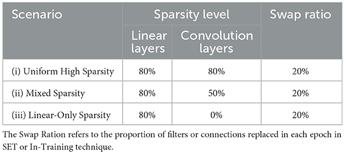
Table 2. Summary of the considered experimental pruning scenarios, including chosen sparsity levels for the different types of layers.

Although choosing sparsity levels is heuristic and depends on the model, dataset, and task complexity, applying different levels of sparsity for different types of layers is a common research practice, as it often yields better results compared to applying the same sparsity level across all layers (Liang et al., 2021; Xiang et al., 2021). Applying these scenarios also allows us to compare the impact of sparsity techniques on different types of layers, such as convolutional and linear layers, providing deeper insights into their behavior.

In other words, when we apply a specific amount of sparsity (e.g., 80%) on the convolutional layers, it means that we remove 80% of the filters in each convolution layer and extract features using the remaining filters. For linear layers, which are only used in the classification part of the models, we remove a specific amount of the total connections (e.g., 80%) between neurons and use the remaining neurons to map the input to the output classes. These scenarios allow us to analyze how varying levels of sparsity affect model performance and resource usage. While previous studies (Chen et al., 2023) use GANs for classification tasks, we focus on simpler and more common models like VGG16 and ResNet18.

To ensure fair comparisons across all combinations of models (Section 3.2), datasets (Section 3.3), and pruning techniques (Section 3.1), we employed a constant training configuration. Specifically, each combination was trained three times for 50 epochs with a batch size of 64 and a learning rate of 1e-4. This configuration presented a balanced trade-off between learning speed and stability during training, allowing us to compare the results across all combinations and scenarios.

The results discussed in Section 4 are based on the average values obtained from three independent runs of the experiments. During our experiments, we observed that all three repetitions of each experiment yielded similar results, confirming the consistency and reliability of our findings. To further ensure the validity of the results, especially for metrics sensitive to external factors (such as inference time and energy efficiency), we conducted each round of experiments at different times of the day. This approach minimized the potential impact of background processes or system load variations. The consistent results across the three repetitions allowed us to limit additional rounds of experiments, as the findings were robust and reproducible.

To ensure reproducibility and clarity, Table 3 summarizes all the considered experimental configurations. The Configuration Category column lists the key aspects of our setup: datasets, model architectures, pruning techniques, pruning scenarios (e.g., sparsity levels), evaluation metrics, and hardware setups (HPC clusters and laptops). The Details column provides specific values or descriptions for each category, including training hyperparameters, hardware specifications, and metric definitions. This table serves as a comprehensive reference for replicating our experiments.

Table 3

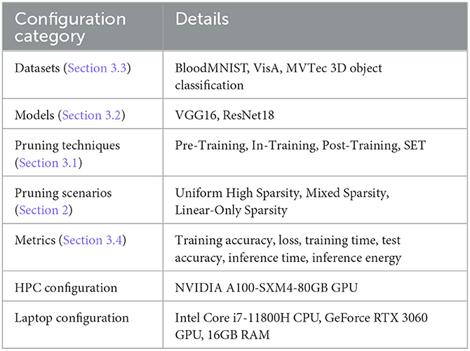
Table 3. Summary of experimental configurations. Categories include datasets, model architectures, pruning methods, hardware setups, and training parameters.

4 Results

In this section, we present and analyze the results of our experiments, focusing on the performance of the sparse models across different pruning techniques and sparsity levels that we discussed in Section 3.5. The results are organized into six subsections, each presenting a specific sight of the model's behavior. First, we investigate training accuracy (Section 4.1), which reflects the model's accuracy at the end of each training epoch. Next, we explore training loss (Section 4.2), which tracks the loss value during each training round, providing insights into the model's learning progress and helping us to prevent the overfitting issue during the training process. The Test accuracy (Section 4.4), shows the final accuracy of the model after training, highlighting its ability to generalize to unseen data. after that, we monitor total training time (Section 4.3), which measures the overall time required to train the model, with further details available in Section 3.4. In addition, we investigate average inference time (Section 4.5), which presents the time the model takes to classify inputs and produce predictions. Besides that, we measured the total training energy for each experiment in Section 4.6. Finally, in Section 4.7, we evaluate the performance of our model on a resource-constrained setting by deploying the model on a general-purpose laptop.

4.1 Training accuracy

Accuracy is a key metric collected during training, evaluated epoch by epoch to compare model performance. Figures 3–5 show the training accuracy varying the pruning fraction. In particular, (i) in Figure 3 all layers had a pruning fraction of 80%, (ii) in Figure 4 only linear layers were pruned at 80% pruning on linear layers while convolutional layers hat a 50% pruning on convolutional layers. Lastly, (iii) in Figure 5 we pruned to 80% only linear layers. The reason behind these scenarios is that using different sparsity levels for different layers is a common practice; for more details, see Section 3.5.

Figure 3

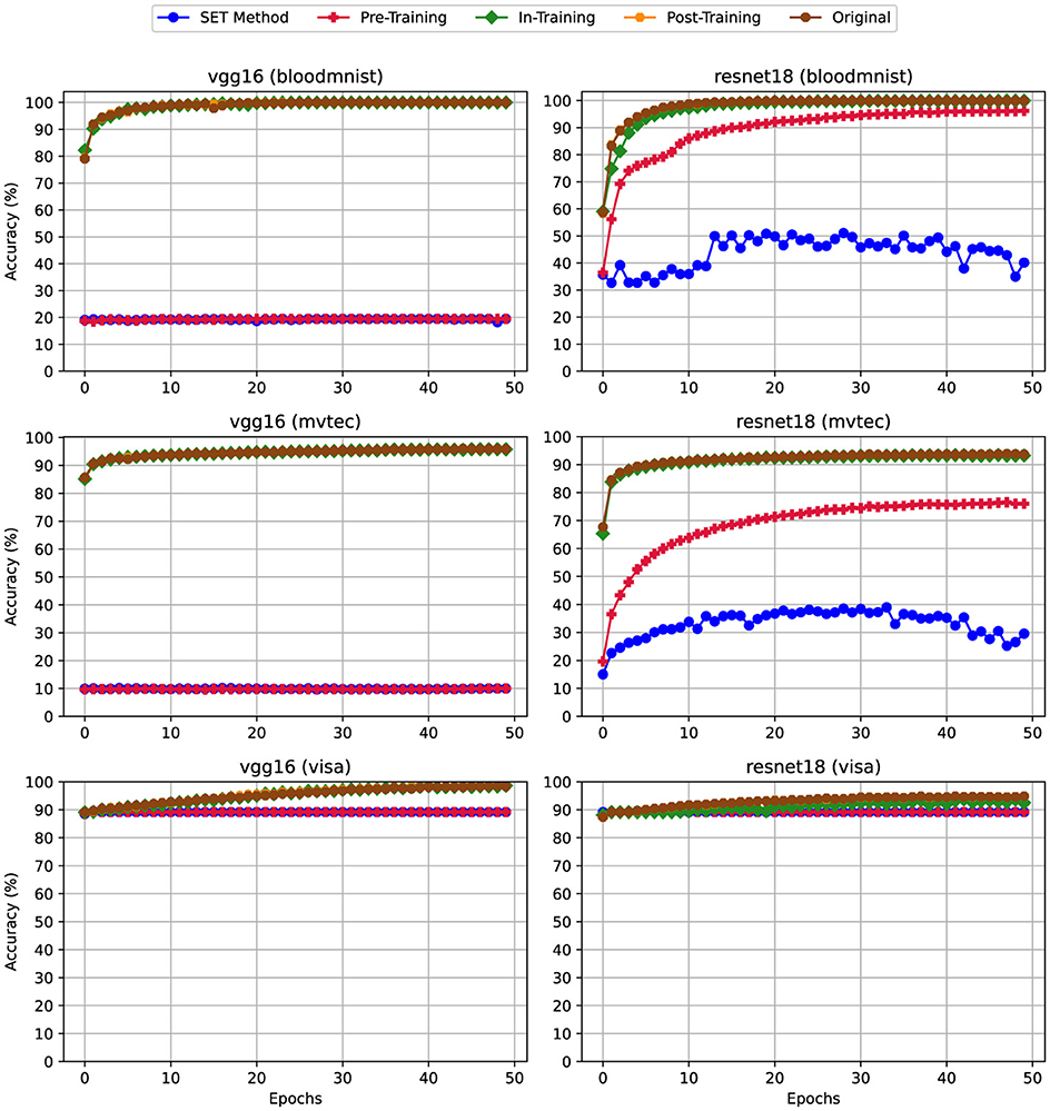
Figure 3. Training Accuracy for scenario (i) Uniform High Sparsity (80%)—Sparsity of 80% applied uniformly to both convolutional and linear layers. For details on all sparsity configurations, refer to Table 2.

Figure 4

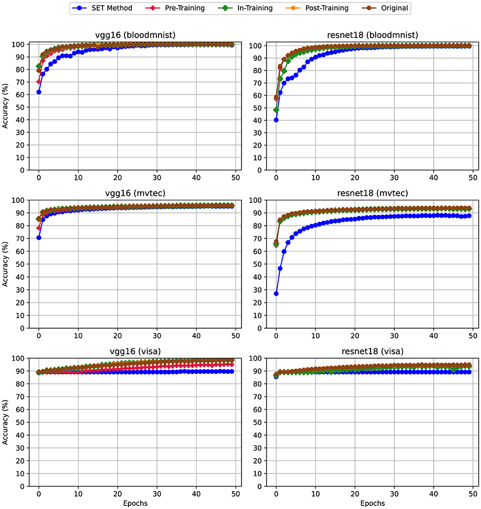
Figure 4. Training Accuracy for scenario (ii) Mixed Sparsity (Linear: 80%, Convolutional: 50%)—Sparsity levels of 80% and 50% applied to linear and convolutional layers, respectively. For details on all sparsity configurations, refer to Table 2.

Figure 5

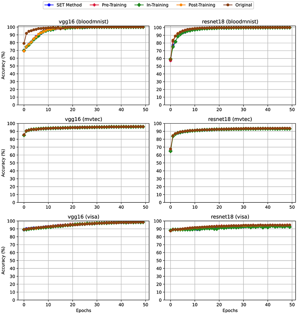
Figure 5. Training Accuracy for scenario (iii) Linear-Only Sparsity—80% sparsity on linear layers, convolutional layers unpruned. For details on all sparsity configurations, refer to Table 2.

From the experiments emerged that applying pruning techniques namely Pre-Training and SET during the training phase impacts the model's accuracy per epoch, particularly due to the sparsity levels applied to the convolutional layers. This effect is observed in both VGG16 and ResNet18 architectures. For example, according to Figure 3, when using VGG16 with the BloodMNIST or MVTec3D datasets, the highest training accuracy achieved was only 20%. In ResNet18, using the same datasets, the best accuracy improves to 50%, but this is still an unsatisfactory result. By reducing the sparsity level of the convolutional layers from 80% in Figure 3 to 50% in Figure 4, the trend of the accuracy for both of these techniques gets closer to the dense version. In Figure 5 we can see that the trend of this metric is mostly matched with the dense version. While this metric for training the same models using the VisA dataset is as good as the dense version, be checking the other metrics like Training Loss in Section 4.2 we can see the effect of applying high sparsity levels on the convolutional layers.

4.2 Training loss

Training loss is another useful metric to evaluate model learning goodness during training. In an ideal scenario, the training loss should decrease gradually over epochs, indicating that the model is minimizing errors and improving its performance. By monitoring the metric we can prevent or detect common errors, especially overfitting, where the model memorizes the training data instead of learning the features and patterns. In other words, if this metric dropped rapidly at the beginning of the training phase we can take this behavior as a sign of this issue. Similarly, if the training loss begins to fluctuate around specific values rather than decreasing, it shows that the model has stopped improving. Both behaviors highlight potential issues in the learning process that need to be addressed.

Like Training Accuracy discussed in Section 4.1, training loss is similarly displayed in Figure 6 (80% pruning on all layers), Figure 7 (80% pruning on linear layers and 50% pruning on convolutional layers), and Figure 8 (80% pruning only on linear layers).

Figure 6

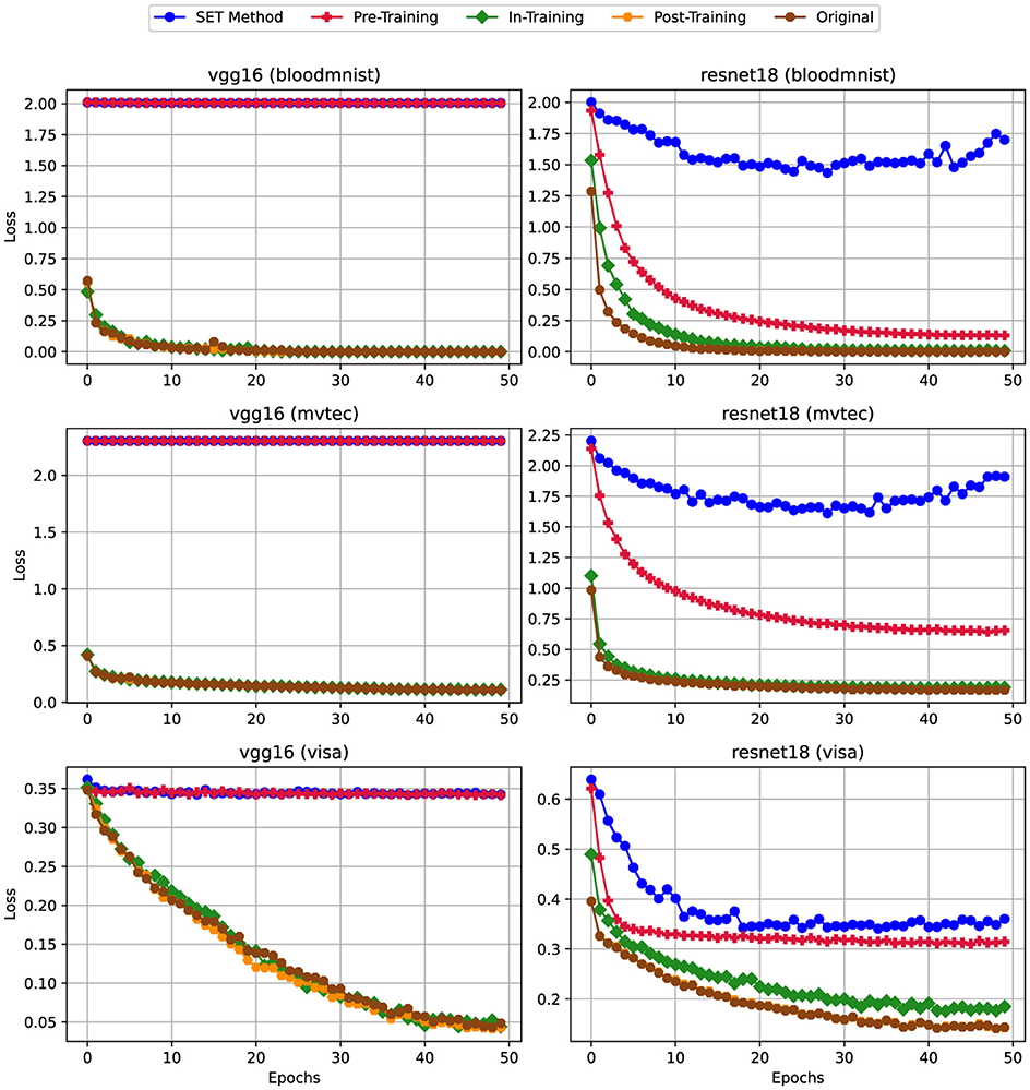
Figure 6. Training Loss for scenario (i) Uniform High Sparsity (80%)—Sparsity of 80% applied uniformly to both convolutional and linear layers. For details on all sparsity configurations, refer to Table 2.

Figure 7

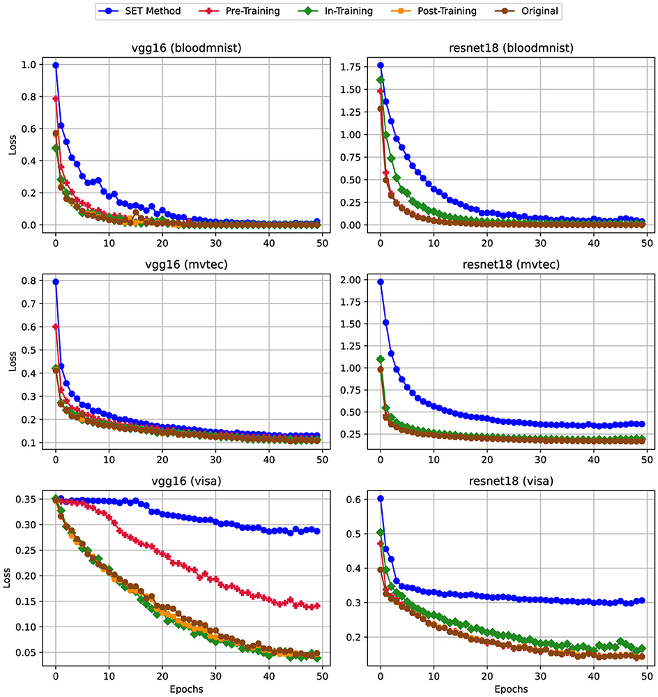
Figure 7. Training Loss for scenario (ii) Mixed Sparsity (Linear: 80%, Convolutional: 50%)—Sparsity levels of 80% and 50% applied to linear and convolutional layers, respectively. For details on all sparsity configurations, refer to Table 2.

Figure 8

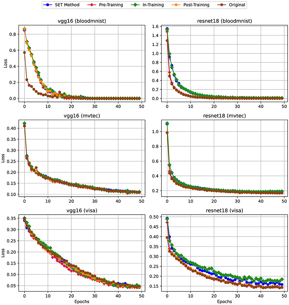
Figure 8. Training Loss for scenario (iii) Linear-Only Sparsity—80% sparsity on linear layers, convolutional layers unpruned. For details on all sparsity configurations, refer to Table 2.

According to the charts, similar to the trends observed in training accuracy, applying pruning techniques like In-Training and SET to dense models impacts the training loss, particularly at higher sparsity levels in Figure 6. For instance, when training VGG16 on the BloodMNIST and MVTec3D datasets, the training loss remains constant, posing around 2. In contrast, that of the VisA dataset fixes at a much lower value (i.e., approximately 0.35), though the general behavior remains consistent across datasets.

On the other hand, reducing the sparsity level from 80% (Figure 6) to 50% (Figure 7) on the convolutional layers leads to significant improvements in the training loss metric. As shown in the charts, except for the VisA dataset, the training loss exhibits a steady decrease from epoch 1 to epoch 50. Finally, in Figure 8, by removing the sparsity from convolutional layers we can see the trend of this metric is getting similar to the dense version.

4.3 Training time

To evaluate model efficiency it is also important to monitor the training time. In industrial settings is particularly important, given that computational resources are limited and expensive. Training time for sparse networks can vary depending on the pruning technique used. For instance, with SET and In-Training methods, we expect an increase in training time since these techniques need to identify weak connections during each epoch. By contrast, Pre-Training and Post-Training methods only need to find these connections once, which results in lower computational overhead. In addition, for the Post-Training technique, if we need to have models with different sparsity levels, we do not need to retrain the model and we can use the dense version again. Moreover, it is important to note that time-based metrics, such as training time, are highly sensitive and can be influenced by both direct and indirect factors. Direct factors include dataset size, image resolution, and model architecture, while indirect factors include the number of parallel tasks competing for resources or background processes running on the system, these kinds of variables can lead to some unexpected behaviors in the experiments. Figures 9–11 show the training time in the three pruning settings.

Figure 9

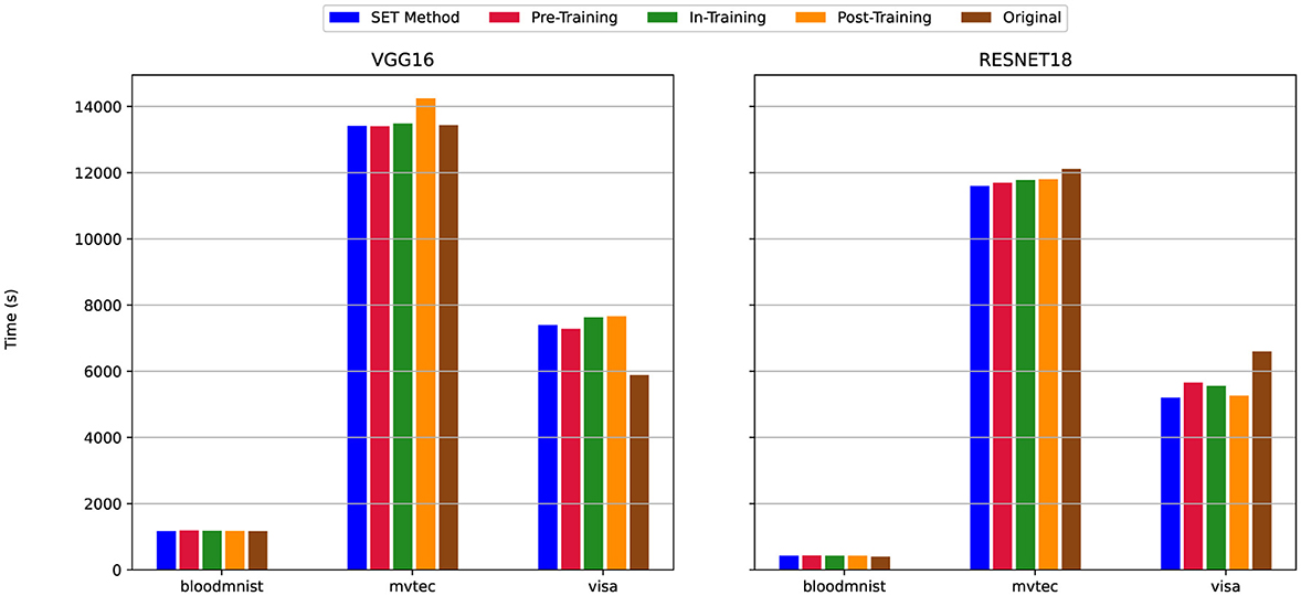
Figure 9. Total Training Time for scenario (i) Uniform High Sparsity (80%)—Sparsity of 80% applied uniformly to both convolutional and linear layers. For details on all sparsity configurations, refer to Table 2.

Figure 10

Figure 10. Total Training Time for scenario (ii) Mixed Sparsity (Linear: 80%, Convolutional: 50%)—Sparsity levels of 80% and 50% applied to linear and convolutional layers, respectively. For details on all sparsity configurations, refer to Table 2.

Figure 11

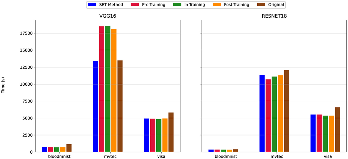
Figure 11. Total Training Time for scenario (iii) Linear-Only Sparsity—80% sparsity on linear layers, convolutional layers unpruned. For details on all sparsity configurations, refer to Table 2.

The figures show that in the majority of cases-85 out of 90 experiments (94% of cases), the training time for SET methods is either comparable to or less than that of dense models, regardless of the model (VGG16 or ResNet18) or dataset used. However, with VGG16 on MVTec3D dataset and an 80% of pruning only for linear layers (Figure 11) the training time for the SET method is similar to the dense version, while the other pruning techniques need more time to complete the training process. Moreover, by training the model with the VisA dataset and VGG16 architecture and the sparsity level set at 80% for both the classification and feature extraction part of the model (Figure 9), the training time for all pruning techniques needs more time compared to the dense version. In this scenario, by changing the model from VGG16 to ResNet18 we have the opposite results and the total training time for the dense version is more than that of sparse models. According to Figure 9, the dense version of the models shows a 500-second increase, while the four other sparse models decrease from nearly 8,000 seconds to 5,800 seconds.

Across all three sets of charts, ResNet18, despite having more convolutional layers than VGG16 (Figure 1), requires less total training time both with and without pruning techniques. The only exception is when training on the VisA dataset, where the difference in training time between VGG16 and ResNet18 becomes insignificant, which shows that, the architecture of this network is more time-efficient compared to VGG16, because of using Residual Block instead of regular convolution blocks.

4.4 Test accuracy

The Test Accuracy results are illustrated across three sets of charts, each of them indicates the specific pruning scenario: Figure 12 presents the 80% pruning on all layers, Figure 13 shows the 80% pruning on linear layers and 50% pruning on convolutional layers, and Figure 14 illustrates the 80% pruning only on linear layers.

Figure 12

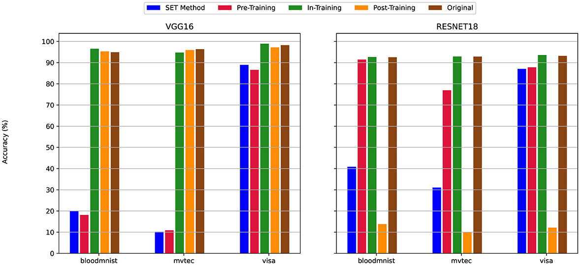
Figure 12. The Test Accuracy for scenario (i) Uniform High Sparsity (80%)—Sparsity of 80% applied uniformly to both convolutional and linear layers. For details on all sparsity configurations, refer to Table 2.

Figure 13

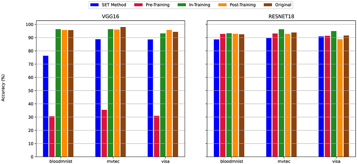
Figure 13. The Test Accuracy for scenario (ii) Mixed Sparsity (Linear: 80%, Convolutional: 50%)—Sparsity levels of 80% and 50% applied to linear and convolutional layers, respectively. For details on all sparsity configurations, refer to Table 2.

Figure 14

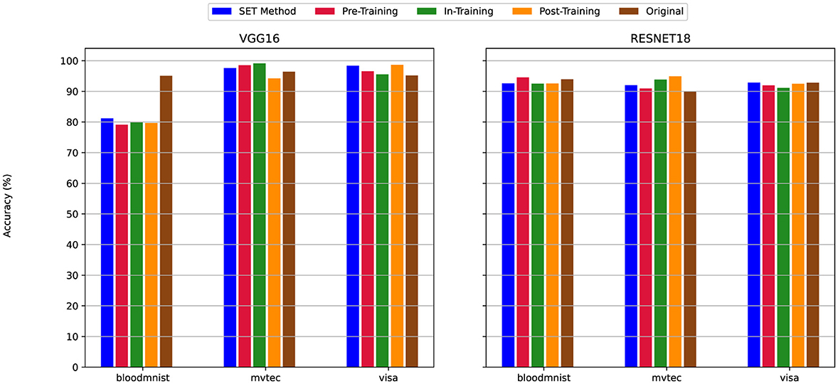
Figure 14. The Test Accuracy for scenario (iii) Linear-Only Sparsity—80% sparsity on linear layers, convolutional layers unpruned. For details on all sparsity configurations, refer to Table 2.

By decreasing the sparsity level in convolution layers from 80% (Figure 12) to 50% (Figure 13), the test accuracy of the SET Method was improved across all datasets and models. For example, when we train the VGG16 with the MVTec3D dataset If we apply the 80% sparsity on both convolution and linear layers (Figure 12) we will have nearly 10% accuracy, even if we change the model to ResNet18 we cannot get better result higher than 30%. However, By decreasing the sparsity level to 50% in convolution layers in Figure 13 the final accuracy of the model for both VGG16 and ResNet18 improved significantly and to nearly 90%. Additionally, if we set the sparsity level at 0% for convolution layers, the accuracy of the model is similar to the dense version. In this scenario (Figure 14), we have an insignificant difference between the accuracy of all the pruning techniques and their dense versions-which is almost 92%.

Moreover, Figure 12 presents that, while changing the models from VGG16 to ResNet18 boosts the accuracy of the models in all the pruning techniques, the opposite change is observed when we apply the 80% sparsity at all the convolution layers by choosing the Post-Training techniques for the sparsification.

According to the the behavior of the models when we decrease the applied sparsity level on the convolution layers, the test accuracy boosts up throughout all experiments. For instance, Figure 12 presents the accuracy of the Pre-Training methods less than 20% when we train the VGG16 model using MVTec3D. However, Figure 14 shows over 90% for the same experiments, with the same configuration.

4.5 Average inference time

Inference time is another metric to determine how fast the trained model can process the data at test time when the training process is finished. The “Average” word, refers to the fact that like the other metrics that we collect after the training finished, we calculate this metric by measuring the total inference time for all the samples that we used for this phase. As shown in Figure 2, we use 20% of VisA and 10% of the BloodMNIST and MVTec3D data set for the test phase and calculate the average inference time between them.

According to this metric, the highest average inference time (slowest) is 0.008s, while the lowest average inference time (fastest) is 0.002s. In the majority of cases–12 out of 18 experiments (75% of cases)—the average inference time for the SET method matches that of the dense version, demonstrating its efficiency. For the remaining 25% of experiments, the SET method exhibits a slightly higher inference time, with a maximum increase of only 0.002s. This light difference remains well within acceptable limits for real-world applications, highlighting the feasibility of the SET method. It is important to note, however, that this experiment did not specifically target real-time applications, leaving an area for future exploration in scenarios with lower latency requirements.

4.6 Total training energy

Energy efficiency is one of the primary metrics when measuring the viability of sparse neural networks, especially in industrial applications where sustainability and resource constraints are crucial. Sparse networks train to reduce computational complexity by removing less important connections, which directly impact the energy required for training. By collecting the total energy usage during the training process, we can evaluate the benefit of pruning techniques in reducing energy usage while maintaining model performance. This metric is particularly important for edge devices and IoT systems (Sofianidis et al., 2024), where energy efficiency is a key for deployment according to their limited power supply (Kang and Lim, 2024).

The total training energy results are organized into three sets of charts, each of them shows the specific pruning scenario: Figure 15 presents the 80% pruning on all layers, Figure 16 shows the 80% pruning on linear layers and 50% pruning on convolutional layers, and Figure 17 illustrates the 80% pruning only on linear layers.

Figure 15

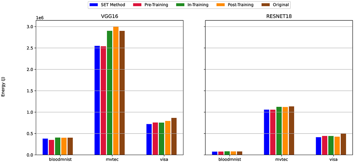
Figure 15. Energy efficiency of sparse vs. dense models under scenario (i) Uniform High Sparsity (see Table 2). Compares energy consumption between sparse (80% sparsity on convolutional and linear layers) and dense models, emphasizing energy savings achieved through pruning while maintaining accuracy.

Figure 16

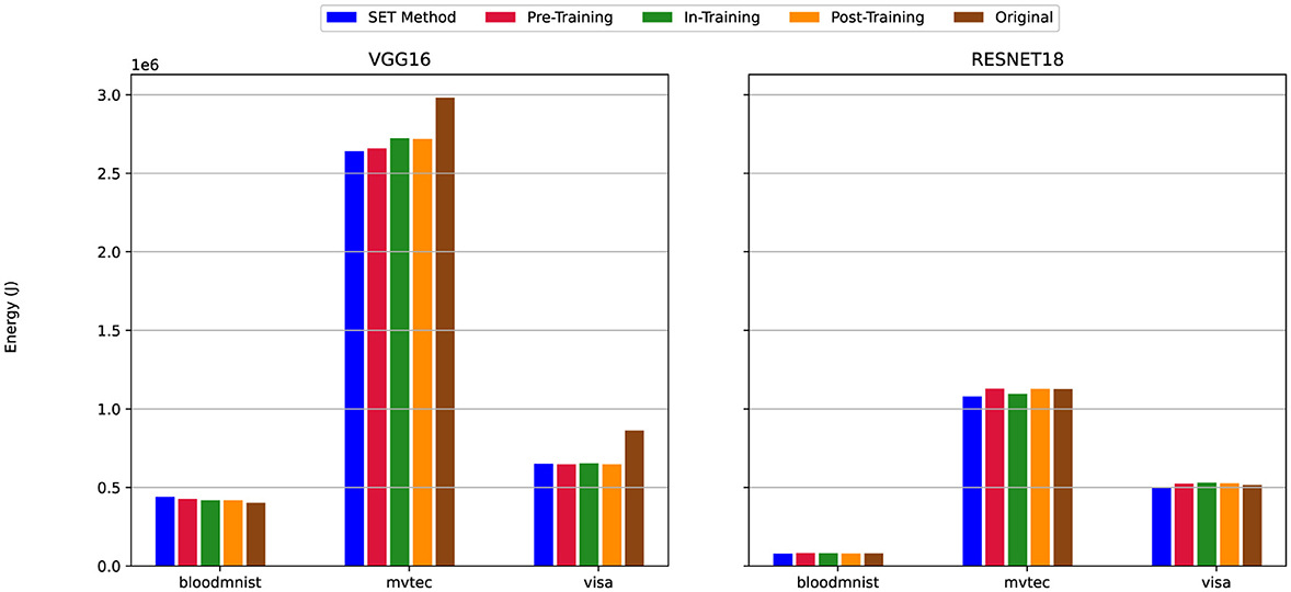
Figure 16. Energy efficiency of sparse vs. dense models under scenario (ii) Mixed Sparsity (see Table 2). Evaluates energy usage for sparse models with 80% sparsity on linear layers and 50% on convolutional layers, demonstrating the trade-offs between energy reduction and performance retention.

Figure 17

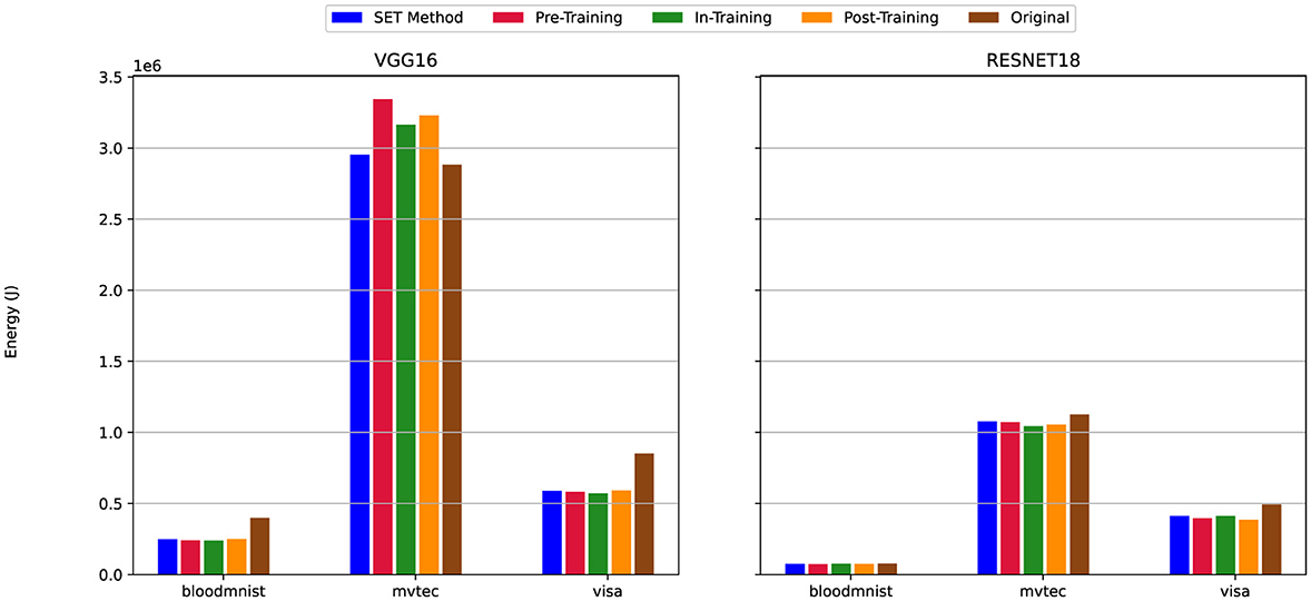
Figure 17. Energy efficiency of sparse models with pruning confined to classification layers in scenario (iii) (see Table 2). Analyzes energy savings when sparsity (80%) is applied exclusively to linear (classification) layers, while convolutional layers remain dense, preserving feature extraction capabilities.

Across all six plots, the SET method consistently indicates better energy efficiency compared to the dense version of the model. Regardless of the dataset (MVTec3D, BloodMNIST, or VisA) (Section 3.3) or the model architecture (VGG16 or ResNet18) (Section 3.2), the SET method requires less energy to train the sparse network. This is observable across all pruning scenarios, as the SET method shows better performance in terms of energy consumption under similar settings and configurations.

Regarding model architecture, ResNet18 always shows better performance compared to VGG16. The difference between training the models using VGG16 or ResNet18 is observable in Figures 15–17 when we choose BloodMNIST and MVTec3D as a dataset to train the model. In detail, when training on the MVTec3D dataset, the average total energy consumption for VGG16 is approximately 2.7 × 10⁶ J across all sparse and dense models, while ResNet18 consumes notably less energy, averaging around 1.1 × 10⁶ J. Furthermore, we observed the same trends for the BloodMNIST dataset, where the average total energy consumption for VGG16 is approximately 0.6 × 10⁶ J, compared to 0.2 × 10⁶ J for ResNet18.

However, between all these illustrations, we have some exceptions. For instance in Figure 15 when training VGG16 on the MVTec3D dataset, the total energy consumption for the In-Training and Post-Training pruning techniques is nearly the same as that of the dense version and higher than that of Pre-Training and SET method. Similarly, another exception occurs in Figure 17, for the same dataset (i.e., MVTec3D) and also the same model (i.e., VGG16), the total energy to train sparse model when we use Pre-Training, In-Training, and Post-Training is higher than Dense and SET method.

4.7 Performance evaluation on resource-constrained devices

Understanding how machine learning models perform on resource-constrained laptop devices is important for real-world applications, where computational resources are limited. To address this, we conducted experiments on a consumer-grade laptop to evaluate the efficiency of sparse neural networks compared to their dense counterparts. These measurements provide insights into the feasibility of deploying such models in resource-constrained environments.

For our experiments, we used a Lenovo Legion 5 laptop, a mid-range consumer device with specifications that can reflect typical hardware available in constrained scenarios (when considering laptops as part of an Edge scenario). This setup mirrors the configuration described in Section 3.5 for consistency, allowing a direct comparison between high-performance computing environments and a more resource-constrained one. According to Table 3, although the Lenovo Legion 5 is a laptop equipped with an NVIDIA GeForce RTX 3060 GPU and an Intel Core i7 CPU, it remains a suitable choice for an initial evaluation of model performance for resource-constrained devices. This is because, in this experiment, we did not use the GPU as our main computational unit, but rather the CPU which is better aligned with the category of resource-constrained environments. Even if the GPU was to be utilized, its performance would not be comparable to high-end GPU processors typically found in HPC or workstation environments. However, the chosen laptop is indeed more powerful than traditional IoT devices such as a Raspberry Pi, but in an industrial setting, it is not necessarily the rule that we only encounter very resource-constrained devices. Nevertheless, this choice allows us to run a variety of experimental scenarios and test and analyse the performance of SNNs compared to their dense counterparts in a timely manner, while doubling as a validation approach for further future experiments. The results indicate that further deployment in more resource-constrained environments should be possible and promising. Besides that, while the Lenovo Legion 5 is not a specialized lightweight device, its affordability and widespread availability make it a suitable proxy for evaluating performance in an initial comparative study of Neural Network pruning strategies. However, in future work, we intend to further address the issue of resource-constrained environments by evaluating and comparing the performance of pruning techniques, alongside assessing the viability of using and training SNNs in a variety of lightweight and very lightweight devices.

We focused on two key metrics that were previously measured in the HPC environment, namely inference time and energy consumption. Inference time was measured as the average duration required to process input samples, excluding the initial model loading phase. Since loading the model is a one-time task, skipping this step allows us to isolate the repetitive computational tasks during inference, which is more relevant for real-time applications. We use average duration to make the results more comparable together since we have different datasets, and the number of samples in each of them is different so by measuring the average time we neutralize the impact of different numbers of samples in the test phase for each dataset.

Energy consumption was, instead, measured for the entire inference process, including both model loading and sample classification, to measure the total energy requirement during the usage.

Measuring inference time helps us evaluate how quickly the model can predict the answers. Faster inference is crucial for applications requiring immediate responses, such as autonomous systems or interactive tools. According to Figure 18, in all our tests, the dense model took longer to process inputs compared to the sparse version. This difference became more noticeable as the sparsity level increased, directly linking sparsity to reduced computational overhead. For instance, a model with 80% sparsity showed faster inference times than a 50% sparse model, reinforcing the benefits of sparsity in optimizing speed. However, finding the best combination between the sparsity level and accuracy of the model is heuristic and depends on our final needs or ultimate goals.

Figure 18

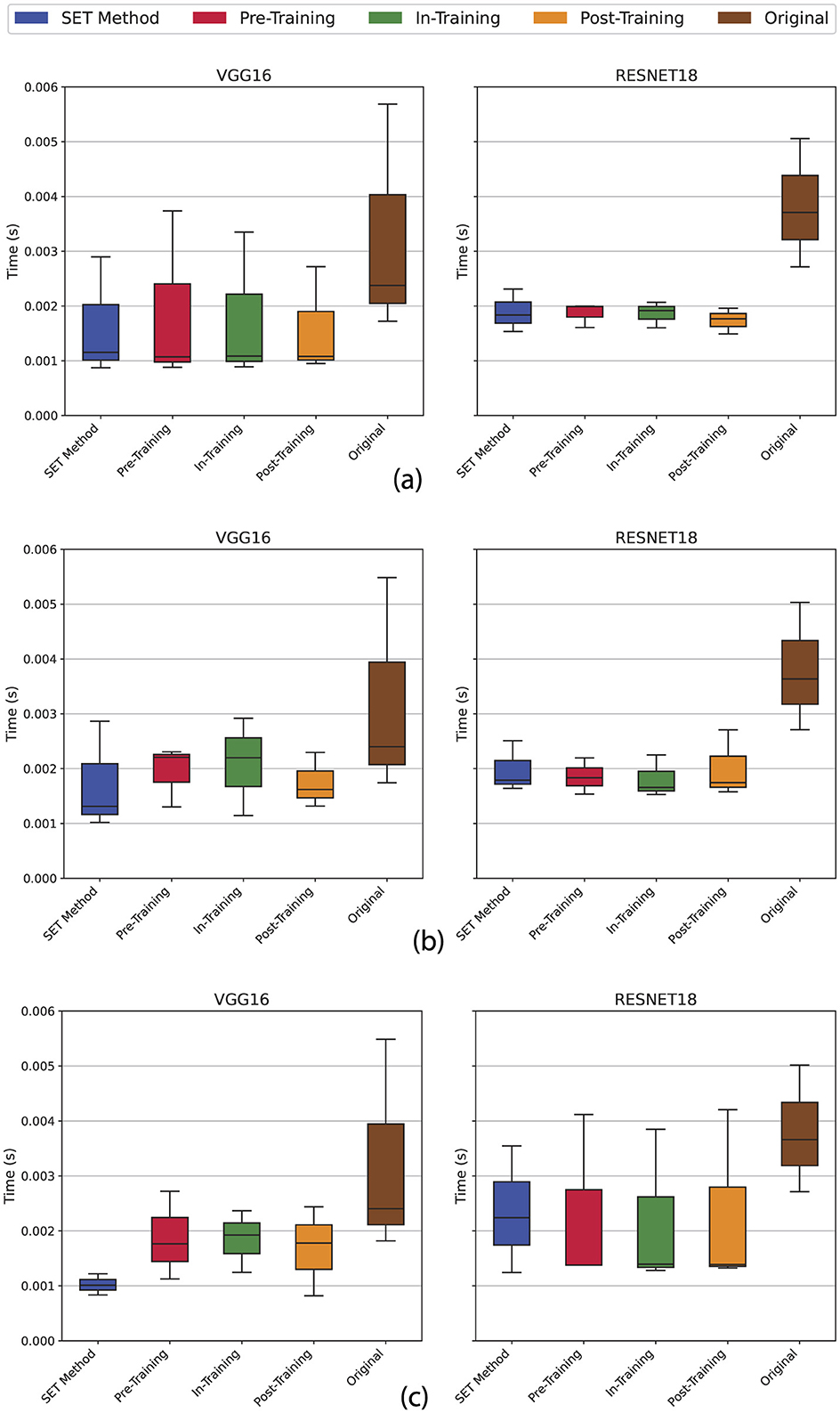
Figure 18. The evaluation of inference time metric on lightweight devices with limited resources based on 3 different sparsity scenarios (see Table 2). (a) Scenario (i), Uniform 80% sparsity applied to both convolution and linear layers; (b) Scenario (ii), Mixed sparsity with 80% on linear layers and 50% on convolution layers; (c) Scenario (iii), Linear-only sparsity (80%) sparsity on linear layers with dense (unpruned) convolution layers.

As expected, minor fluctuations were observed in the experimental results. These variations primarily come from the use of general-purpose devices (e.g., consumer laptops) during evaluation, which essentially runs background processes for routine user tasks. Fully deactivating these processes is impractical, as such devices prioritize multitasking over-controlled, isolated workloads. In contrast, real-world IoT deployments usually involve dedicated devices optimized for specific tasks. In these scenarios, administrators retain full control over resource allocation, enabling the model to utilize the device's computational capacity exclusively, thereby minimizing interference and stabilizing performance. This distinction highlights the importance of context-aware evaluations when assessing models for lightweight or edge-computing applications.

Energy consumption is equally important, especially for battery-powered devices. Our experiments realize that energy usage depends on the model architecture. According to Figure 19, VGG-based models require more energy to load and run compared to ResNet-based designs (Lazzaro et al., 2023; Canziani et al., 2016). This trend aligns with our earlier observations on HPC systems, where VGG architectures demanded higher computational resources. One of the main reason behind this difference is that in VGG16 model has 138,000,000 parameters while the ResNet18 has only 11,000,000 parameters. The other reason also is that in ResNet-based model have residual blocks and skip connections in their architecture, while in VGG-based model we use the regular convolution layers. It is worth to mention that the sparse versions of both architectures used less energy than their dense counterparts. However, the impact of energy reduction on the sparse version of the model is not as much as we expected, and we believe that this difference is related to the how PyTorch library implements the sparsification. This library uses a mask Matrix to generate the final model and in this way, parts of the prunned connection still exist and it affects the energy metric during the inference phase. This reduction highlights how sparsity not only improves inference time but also lowers energy costs, making sparse models more sustainable for deployment in resource-limited scenarios and environments.

Figure 19

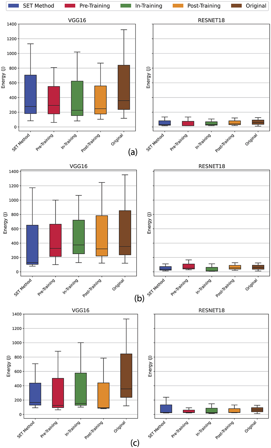
Figure 19. The evaluation of total energy consumption metric on lightweight devices with limited resources based on 3 different sparsity scenarios (see Table 2). (a) Uniform 80% sparsity applied to both convolution and linear layers; (b) Mixed sparsity with 80% on linear layers and 50% on convolution layers; (c) Linear-only sparsity (80%) sparsity on linear layers with dense (unpruned) convolution layers.

These findings confirm that the advantages of sparse networks observed in HPC environments extend to lightweight devices. The consistent reduction in inference time and energy consumption across both settings underscores the robustness of our experiments. This evaluation fills the gap between theoretical efficiency and real-world usage.

5 Discussion

The performed experiments led us to a number of insightful observations. According to the results, applying high levels of sparsity to convolutional layers significantly impacts the final accuracy of the model. We observed that increasing the sparsity level from 50% to 80% on convolutional layers can reduce the final accuracy by up to 80% in the worst-case scenario of our experiments, as illustrated in Figure 12. This highlights the critical role of convolutional layers in feature extraction and also the role of each filter in extracting the features from inputs during the training process.

By contrast, applying the same level of sparsity (80%) to linear layers, which are the main component of the models' classification part, does not significantly impact the final accuracy. In our experiments, when sparsity techniques were applied to linear layers in the classification component, we achieved comparable results in 87.5% of all cases (21 out of 24 sparse models), indicating that sparse networks can maintain performance close to that of dense models when sparsity is limited to linear layers, as visualized in Figure 14.

This observation confirms our expectation: while applying a higher sparsity level to the linear layers of the model does impact the final accuracy, the high number of connections in this part of the model covers the removed connections. For instance, the large number of connections in linear layers allows the model to maintain robust performance even after pruning, as the remaining connections can effectively redistribute the information flow.

Training time is one of the key metrics that directly impacts total energy usage. By comparing similar experiments, we can identify the reasons behind the exceptions in total energy consumption discussed in Section 4.6. According to the charts, the total training time for VGG16 trained on the MVTec3D dataset is higher when using Pre-Training, In-Training, and Post-Training techniques compared to the SET method and the dense version of the model, which is matched with the same behavior of energy consumption. This increased training time leads to higher energy consumption. However, this discrepancy in training time may also be attached to indirect factors, such as background processes, hardware architecture, or the use of virtual GPU partitions instead of dedicated hardware (for more details, see Section 3).

As confirmed by the energy consumption metric, our experiments show that the pruned versions of the models are more energy-efficient compared to their dense versions, which highlights a key advantage of pruning: reducing computational overhead while keeping model performance. However, contrary to our expectations, increasing the sparsity level did not consistently lead to further reductions in energy consumption. We attribute this to the implementation of sparsification in PyTorch, which uses mask matrix for filters and weights during training. In this approach, increasing the sparsity level only modifies the mask values during the training stage. Despite this limitation, our work showcases the potential of pruning to improve energy efficiency.

6 Conclusion

In this paper, we investigate the performance of different pruning techniques for industrial applications, to achieve this goal we used two of the most common model architectures including VGG16 and ResNet18 in the industrial environment. We commence with similar works in the industrial environment and the other papers that used similar models, datasets, or pruning techniques. Then we define sparse neural networks and explain the pruning techniques used in our experiments. After that, we explain the architecture of the models and dataset that we used in detail. Finally, we collect metrics to evaluate the performance of sparse networks in industrial settings, focusing on energy efficiency, accuracy, and inference time. By collecting these metrics, we compared the effectiveness of different pruning techniques, including the SET method in the same environment, and examined their impact on model performance and energy consumption.

According to the results, although using common machine learning libraries in an industrial environment, i.e., PyTorch, to develop and implement our experiments introduces limitations–such as relying on mask matrices to create pruned models and constraints on modifying the model architecture during training–we successfully show reductions in total energy consumption during the training phase. This is particularly evident when using the SET method to prune the network, which consistently outperformed three other pruning techniques that we used for our experiments in terms of energy efficiency. The SET method's strong approach to sparsity, which keeps the most important connections in linear layers and filters in convolution layers while pruning weaker ones in each training round, confirms highly efficient for industrial applications where energy efficiency is crucial and leads to cost reduction on large-scale cases.

Moreover, while the remaining methods also show a decrease in energy consumption during the training stage, the SET method shows better performance in terms of efficiency. Besides that, simpler techniques such as Post-Training pruning require major attention, as they inherit the drawbacks of the dense model. For instance, if the dense version of the model suffers from overfitting, the sparse version will retain this issue, limiting its generalization capability. This emphasizes the importance of using stronger pruning techniques that not only reduce energy consumption but also are able to address other weaknesses.

In summary, this research highlights the potential of sparse neural networks, particularly the one that used the pruning of the model during the training namely, the SET method and In-Training, to provide energy-efficient solutions for industrial applications. By addressing the challenges of energy consumption and computational costs, our work clears the way for more sustainable and scalable AI deployments in industrial settings.

7 Future work

While this study provides valuable insights, several areas remain unexplored, offering significant opportunities for further research. One of the potential directions is the integration of sparse neural networks with real-time industrial systems. Fault detection is a critical element of manufacturing pipelines, and establishing low-resource, energy-efficient models in this context can notably enhance operational efficiency. By enabling real-time monitoring and lively anomaly detection, sparse models can reduce downtime, decrease production losses, and improve overall output in industrial settings.

Another area for exploration is federated learning with sparse models. This approach can revolutionize how industrial AI systems are trained and deployed. Federated learning allows sparse models to be trained on low-cost devices, such as smartphones or IoT sensors while keeping data privacy. Instead of centralizing data on a single server, each device trains the model locally using its own data and computational resources, and only the model updates (not the raw data) are shared with a central server. This decentralized training pattern not only enhances data privacy but also addresses the challenge of limited datasets in industrial applications. Moreover, federated learning enables collaboration among similar industries by allowing them to collectively improve a single shared model without compromising sensitive data.

We also plan to investigate the efficacy of sparse neural networks in more limited-resource environments such as IoT and edge devices (e.g., Raspberry Pi, NVIDIA Jetson Boards) which is the ultimate goal of our research. These platforms naturally face limitations in computational power, memory, and energy budgets, making sparse architectures a potential candidate for efficient deployment. Additionally, we aim to evaluate the impact of quantization techniques on these sparse models, analyzing how reduced precision affects their accuracy, latency, and energy efficiency. A deeper exploration of the interplay between sparsity and quantization could yield practical insights into optimizing neural networks for real-world applications while maintaining robustness under hardware limitations.

Additionally, future work should expand the comparison of sparse models across heavier datasets, diverse architectures, and more complex models. For instance, evaluating the performance of sparse networks on large-scale industrial datasets, such as high-resolution data or multi-modal datasets, could provide deeper insights into their scalability. Exploring architectures beyond CNNs, such as Transformers or Graph Neural Networks (GNNs), would also help generalize the findings of this study to a broader range of applications.

Data availability statement

Publicly available datasets were analyzed in this study. This data can be found here: https://medmnist.com/, https://www.kaggle.com/datasets/beschue/industrial-classification-data-set/, and https://paperswithcode.com/dataset/visa.

Author contributions

AD: Data curation, Software, Visualization, Writing – original draft. AL: Conceptualization, Supervision, Validation, Writing – review & editing. LE: Investigation, Writing – review & editing. LC: Investigation, Methodology, Supervision, Writing – review & editing.

Funding

The author(s) declare that financial support was received for the research and/or publication of this article. This work was supported by the Open Access Publishing Fund of the Free University of Bozen-Bolzano and was carried out in the context of project COMMON-WEARS (Community oriented wearable computing systems), funded by the Italian Ministry of Research (PRIN 2020 program), grant number I53C21000210001.

Conflict of interest

The authors declare that the research was conducted in the absence of any commercial or financial relationships that could be construed as a potential conflict of interest.

Generative AI statement

The author(s) declare that no Gen AI was used in the creation of this manuscript.

Publisher's note

All claims expressed in this article are solely those of the authors and do not necessarily represent those of their affiliated organizations, or those of the publisher, the editors and the reviewers. Any product that may be evaluated in this article, or claim that may be made by its manufacturer, is not guaranteed or endorsed by the publisher.

Footnotes

1. ^“MedMNIST” dataset: https://medmnist.com/.

2. ^“MVTec 3D Object Classification” Dataset: https://www.kaggle.com/datasets/beschue/industrial-classification-data-set/.

3. ^“VisA” Dataset: https://paperswithcode.com/dataset/visa.

4. ^Available at https://ml.energy/zeus/.

References

Akcay, S., Ameln, D., Vaidya, A., Lakshmanan, B., Ahuja, N., and Genc, U. (2022). “Anomalib: a deep learning library for anomaly detection,” in 2022 IEEE International Conference on Image Processing (ICIP) (IEEE), 1706–1710. doi: 10.1109/ICIP46576.2022.9897283

Crossref Full Text | Google Scholar

Andriulo, F. C., Fiore, M., Mongiello, M., Traversa, E., and Zizzo, V. (2024). Edge computing and cloud computing for internet of things: a review. Informatics (MDPI) 11:71. doi: 10.3390/informatics11040071

Crossref Full Text | Google Scholar

Apostolopoulos, I. D., and Tzani, M. A. (2022). Industrial object and defect recognition utilizing multilevel feature extraction from industrial scenes with deep learning approach. J. Ambient Intell. Humaniz. Comput. 14, 10263–10276. doi: 10.1007/s12652-021-03688-7

Crossref Full Text | Google Scholar

Atashgahi, Z., Liu, T., Pechenizkiy, M., Veldhuis, R., Mocanu, D. C., and van der Schaar, M. (2024). Unveiling the power of sparse neural networks for feature selection. arXiv:2408.04583.

Google Scholar

Balaprakash, P., Egele, R., Salim, M., Wild, S., Vishwanath, V., Xia, F., et al. (2019). “Scalable reinforcement-learning-based neural architecture search for cancer deep learning research,” in Proceedings of the International Conference for High Performance Computing, Networking, Storage and Analysis, SC '19 (New York, NY, USA: Association for Computing Machinery), 33. doi: 10.1145/3295500.3356202

Crossref Full Text | Google Scholar

Blalock, D., Ortiz, J. J. G., Frankle, J., and Guttag, J. (2020). What is the state of neural network pruning? arXiv:2003.03033.

Google Scholar

Brennan, R. L., and Lee, T. (2024). “Extremely low-power edge connected devices,” in 2024 IEEE 67th International Midwest Symposium on Circuits and Systems (MWSCAS) (IEEE), 674–677. doi: 10.1109/MWSCAS60917.2024.10658964

Crossref Full Text | Google Scholar

Canziani, A., Paszke, A., and Culurciello, E. (2016). An analysis of deep neural network models for practical applications. arXiv:1605.07678.

Google Scholar

Chen, X., Han, Y., and Zhang, J. (2023). APRIL-GAN: a zero-/few-shot anomaly classification and segmentation method for CVPR 2023 VAND workshop challenge tracks 1&2: 1st place on zero-shot AD and 4th place on few-shot AD. arXiv:2305.17382.

Google Scholar

Cheng, H., Zhang, M., and Shi, J. Q. (2024). A survey on deep neural network pruning: taxonomy, comparison, analysis, and recommendations. IEEE Trans. Pattern Anal. Mach. Intell. 46, 10558–10578. doi: 10.1109/TPAMI.2024.3447085

PubMed Abstract | Crossref Full Text | Google Scholar

Deng, J., Dong, W., Socher, R., Li, L.-J., Li, K., and Fei-Fei, L. (2009). “Imagenet: a large-scale hierarchical image database,” in 2009 IEEE Conference on Computer Vision and Pattern Recognition (IEEE), 248–255. doi: 10.1109/CVPR.2009.5206848

PubMed Abstract | Crossref Full Text | Google Scholar

Doerrich, S., Di Salvo, F., Brockmann, J., and Ledig, C. (2024). Rethinking model prototyping through the MedMNIST+ dataset collection. Sci. Rep. 15:7669. doi: 10.1038/s41598-025-92156-9

PubMed Abstract | Crossref Full Text | Google Scholar

Drost, B., Ulrich, M., Bergmann, P., Härtinger, P., and Steger, C. (2017). “Introducing mvtec itodd – a dataset for 3d object recognition in industry,” in 2017 IEEE International Conference on Computer Vision Workshops (ICCVW), 2200–2208. doi: 10.1109/ICCVW.2017.257

Crossref Full Text | Google Scholar

Duan, J., Shi, T., Zhou, H., Xuan, J., and Wang, S. (2021). A novel ResNet-based model structure and its applications in machine health monitoring. J. Vib. Control 27, 1036–1050. doi: 10.1177/1077546320936506

Crossref Full Text | Google Scholar

Erdős, P., and Rényi, A. (2022). On random graphs. I. Publ. Math. Debrecen 6, 290–297. doi: 10.5486/PMD.1959.6.3-4.12

PubMed Abstract | Crossref Full Text | Google Scholar

Erhan, L., Liotta, A., and Cavallaro, L. (2025). “Comparing training of sparse to classic neural networks for binary classification in medical data,” in Lecture Notes in Computer Science (Cham: Springer Nature Switzerland), 101–106. doi: 10.1007/978-3-031-78049-3_10

Crossref Full Text | Google Scholar

Gadhikar, A., Mukherjee, S., and Burkholz, R. (2022). Why random pruning is all we need to start sparse. arXiv:2210.02412.

Google Scholar

Gao, H., Zhen, T., and Li, Z. (2022). Detection of wheat unsound kernels based on improved ResNet. IEEE Access 10, 20092–20101. doi: 10.1109/ACCESS.2022.3147838

Crossref Full Text | Google Scholar

Goodfellow, I. J., Pouget-Abadie, J., Mirza, M., Xu, B., Warde-Farley, D., Ozair, S., et al. (2014). Generative adversarial networks. arXiv:1406.2661.

Google Scholar

He, K., Zhang, X., Ren, S., and Sun, J. (2016). “Deep residual learning for image recognition,” in 2016 IEEE Conference on Computer Vision and Pattern Recognition (CVPR) (IEEE), 770–778. doi: 10.1109/CVPR.2016.90

Crossref Full Text | Google Scholar

Hossain, M. S., Al-Hammadi, M., and Muhammad, G. (2019). Automatic fruit classification using deep learning for industrial applications. IEEE Trans. Industr. Inform. 15, 1027–1034. doi: 10.1109/TII.2018.2875149

Crossref Full Text | Google Scholar

Huo, Z., Gu, B., and Huang, H. (2021). Large batch optimization for deep learning using new complete layer-wise adaptive rate scaling. Proc. Conf. AAAI Artif. Intell. 35, 7883–7890. doi: 10.1609/aaai.v35i9.16962

Crossref Full Text | Google Scholar

Jayasimhan, A., and Pabitha, P. (2024). Resprune: an energy-efficient restorative filter pruning method using stochastic optimization for accelerating CNN. Pattern Recogn. 155:110671. doi: 10.1016/j.patcog.2024.110671

Crossref Full Text | Google Scholar

Jeong, J., Zou, Y., Kim, T., Zhang, D., Ravichandran, A., and Dabeer, O. (2023). “Winclip: Zero-/few-shot anomaly classification and segmentation,” in 2023 IEEE/CVF Conference on Computer Vision and Pattern Recognition (CVPR) (IEEE), 19606–19616. doi: 10.1109/CVPR52729.2023.01878

Crossref Full Text | Google Scholar

Kanagarla, K. (2024). Edge computing and analytics for iot devices: enhancing real-time decision making in smart environments. Int. J. Multidisc. Res. 6, 1–9. doi: 10.2139/ssrn.5012466

PubMed Abstract | Crossref Full Text | Google Scholar

Kang, Y.-M., and Lim, Y.-S. (2024). Handling power depletion in energy harvesting IoT devices. Electronics 13:2704. doi: 10.3390/electronics13142704

Crossref Full Text | Google Scholar

Khan, R. U., Zhang, X., Kumar, R., and Tariq, H. A. (2017). “Analysis of resnet model for malicious code detection,” in 2017 14th International Computer Conference on Wavelet Active Media Technology and Information Processing (ICCWAMTIP) (IEEE), 239–242. doi: 10.1109/ICCWAMTIP.2017.8301487

PubMed Abstract | Crossref Full Text | Google Scholar

Kolapo, R., Kawu, F. M., Abdulmalik, A. D., Edem, U. A., Young, M. A., and Mordi, E. C. (2024). Edge computing: revolutionizing data processing for IoT applications. Int. J. Sci. Res. Arch. 13, 023–029. doi: 10.30574/ijsra.2024.13.2.2082

Crossref Full Text | Google Scholar

Krizhevsky, A. (2014). One weird trick for parallelizing convolutional neural networks. arXiv:1404.5997.

Google Scholar

Lasby, M., Golubeva, A., Evci, U., Nica, M., and Ioannou, Y. (2023). Dynamic sparse training with structured sparsity. arXiv:2305.02299.

Google Scholar

Lazzaro, D., Ciná, A. E., Pintor, M., Demontis, A., Biggio, B., Roli, F., et al. (2023). Minimizing energy consumption of deep learning models by energy-aware training. arXiv:2307.00368.

Google Scholar

Lee, J., Lee, Y. C., and Kim, J. T. (2020). Fault detection based on one-class deep learning for manufacturing applications limited to an imbalanced database. J. Manuf. Syst. 57, 357–366. doi: 10.1016/j.jmsy.2020.10.013

Crossref Full Text | Google Scholar

Li, I.-H., and Chang, T.-S. (2024). “Dynamic gradient sparse update for edge training,” in 2024 IEEE International Symposium on Circuits and Systems (ISCAS), 1–5. doi: 10.1109/ISCAS58744.2024.10558072

PubMed Abstract | Crossref Full Text | Google Scholar

Liang, T., Glossner, J., Wang, L., Shi, S., and Zhang, X. (2021). Pruning and quantization for deep neural network acceleration: a survey. Neurocomputing 461, 370–403. doi: 10.1016/j.neucom.2021.07.045

Crossref Full Text | Google Scholar

Lin, T.-Y., Maire, M., Belongie, S., Bourdev, L., Girshick, R., Hays, J., et al. (2014). Microsoft COCO: common objects in context. arXiv:1405.0312.

Google Scholar

Ma, X., Qin, M., Sun, F., Hou, Z., Yuan, K., Xu, Y., et al. (2021). Effective model sparsification by scheduled grow-and-prune methods. arXiv:2106.09857.

Google Scholar

Mittal, D., Bhardwaj, S., Khapra, M. M., and Ravindran, B. (2019). Studying the plasticity in deep convolutional neural networks using random pruning. Mach. Vis. Appl. 30, 203–216. doi: 10.1007/s00138-018-01001-9

Crossref Full Text | Google Scholar

Mocanu, D. C., Mocanu, E., Stone, P., Nguyen, P. H., Gibescu, M., and Liotta, A. (2018). Scalable training of artificial neural networks with adaptive sparse connectivity inspired by network science. Nat. Commun. 9:2383. doi: 10.1038/s41467-018-04316-3

PubMed Abstract | Crossref Full Text | Google Scholar

Nikdan, M., Pegolotti, T., Iofinova, E., Kurtic, E., and Alistarh, D. (2023). SparseProp: Efficient sparse backpropagation for faster training of neural networks. arXiv:2302.04852.

Google Scholar

Nimmagadda, Y. (2025). “Model optimization techniques for edge devices,” in Model Optimization Methods for Efficient and Edge AI, Ch. 4 (John Wiley & Sons, Ltd), 57–85. doi: 10.1002/9781394219230.ch4

Crossref Full Text | Google Scholar

Palena, M., Cerquitelli, T., and Chiasserini, C. F. (2024). Edge-device collaborative computing for multi-view classification. Comput. Netw. 254:110823. doi: 10.1016/j.comnet.2024.110823

Crossref Full Text | Google Scholar

Qu, Y., Qu, L., Chen, T., Zhao, X., Li, J., and Yin, H. (2024). Sparser training for on-device recommendation systems. arXiv:2411.12205.

Google Scholar

Rane, J., Kaya, Ö., Mallick, S. K., and Rane, N. L. (2024). “Scalable and adaptive deep learning algorithms for large-scale machine learning systems,” in Future Research Opportunities for Artificial Intelligence in Industry 4.0 and 5.0 (Deep Science Publishing), 39–92. doi: 10.70593/978-81-981271-0-5_2

Crossref Full Text | Google Scholar

Redmon, J., Divvala, S., Girshick, R., and Farhadi, A. (2016). “You only look once: unified, real-time object detection,” in 2016 IEEE Conference on Computer Vision and Pattern Recognition (CVPR) (IEEE), 779–788. doi: 10.1109/CVPR.2016.91

PubMed Abstract | Crossref Full Text | Google Scholar

Reed, R. (1993). Pruning algorithms-a survey. IEEE Trans. Neural Netw. 4, 740–747. doi: 10.1109/72.248452

PubMed Abstract | Crossref Full Text | Google Scholar

Schuerrle, B., Sankarappan, V., and Morozov, A. (2023). “SynthiCAD: generation of industrial image data sets for resilience evaluation of safety-critical classifiers,” in Proceeding of the 33rd European Safety and Reliability Conference (Singapore: Research Publishing Services), 2199–2206. doi: 10.3850/978-981-18-8071-1_P400-cd

Crossref Full Text | Google Scholar

Shi, Y., Tang, A., Niu, L., and Zhou, R. (2024). Sparse optimization guided pruning for neural networks. Neurocomputing 574:127280. doi: 10.1016/j.neucom.2024.127280

Crossref Full Text | Google Scholar

Shuvo, M. M. H., Islam, S. K., Cheng, J., and Morshed, B. I. (2023). Efficient acceleration of deep learning inference on resource-constrained edge devices: a review. Proceed. IEEE 111, 42–91. doi: 10.1109/JPROC.2022.3226481

Crossref Full Text | Google Scholar

Simonyan, K., and Zisserman, A. (2014). Very deep convolutional networks for large-scale image recognition. arXiv:1409.1556.

Google Scholar

Sofianidis, I., Konstantakos, V., and Nikolaidis, S. (2024). “Energy consumption aspects on embedded system for IoT applications,” in 2024 13th International Conference on Modern Circuits and Systems Technologies (MOCAST) (IEEE), 1–5. doi: 10.1109/MOCAST61810.2024.10615490

PubMed Abstract | Crossref Full Text | Google Scholar

Soumyalatha, N., and Manjunath, R. K. (2023). Compact optimized deep learning model for edge: a review. Int. J. Electr. Comput. Eng. 13:6904. doi: 10.11591/ijece.v13i6.pp6904-6912

Crossref Full Text | Google Scholar

Sun, C., Chen, J., Li, Y., Wang, W., and Ma, T. (2023). Random pruning: channel sparsity by expectation scaling factor. PeerJ Comput. Sci. 9:e1564. doi: 10.7717/peerj-cs.1564

PubMed Abstract | Crossref Full Text | Google Scholar

Susskind, Z., Arora, A., Miranda, I. D. S., Bacellar, A. T. L., Villon, L. A. Q., Katopodis, R. F., et al. (2023). ULEEN: a novel architecture for ultra low-energy edge neural networks. arXiv:2304.10618.

Google Scholar

Taha, R. T., Abdullah, A. O., Dronach, A., Shnain, S. K., Khaleefah, A. M., and Tkachenko, O. (2024). “The convergence of edge computing and IoT-A paradigm shift in data processing,” in 2024 36th Conference of Open Innovations Association (FRUCT) (IEEE), 787–796. doi: 10.23919/FRUCT64283.2024.10749961

Crossref Full Text | Google Scholar

Tyche, N., Taylor, A., Evans, J., and Reid, M. (2024). Improving neural network efficiency through advanced pruning techniques. Techrxiv. doi: 10.36227/techrxiv.172720330.08872446/v1

Crossref Full Text | Google Scholar

Wang, J. (2023). Research on pruning optimization techniques for neural networks. Appl. Comput. Eng. 19, 152–158. doi: 10.54254/2755-2721/19/20231025

Crossref Full Text | Google Scholar

Witt, N., Deutel, M., Schubert, J., Sobel, C., and Woller, P. (2024). “Energy-efficient AI on the edge,” in Unlocking Artificial Intelligence (Cham: Springer Nature Switzerland), 359–380. doi: 10.1007/978-3-031-64832-8_19

Crossref Full Text | Google Scholar

Wu, S., Li, G., Deng, L., Liu, L., Wu, D., Xie, Y., et al. (2019). L1 -norm batch normalization for efficient training of deep neural networks. IEEE Trans. Neural Netw. Learn. Syst. 30, 2043–2051. doi: 10.1109/TNNLS.2018.2876179

PubMed Abstract | Crossref Full Text | Google Scholar

Xiang, K., Peng, L., Yang, H., Li, M., Cao, Z., Jiang, S., et al. (2021). A novel weight pruning strategy for light weight neural networks with application to the diagnosis of skin disease. Appl. Soft Comput. 111:107707. doi: 10.1016/j.asoc.2021.107707

Crossref Full Text | Google Scholar

Xu, W., Fu, Y.-L., and Zhu, D. (2023). ResNet and its application to medical image processing: research progress and challenges. Comput. Methods Progr. Biomed. 240:107660. doi: 10.1016/j.cmpb.2023.107660

PubMed Abstract | Crossref Full Text | Google Scholar

Yang, J., Shi, R., and Ni, B. (2021). “Medmnist classification decathlon: a lightweight automl benchmark for medical image analysis,” in 2021 IEEE 18th International Symposium on Biomedical Imaging (ISBI) (IEEE), 191–195. doi: 10.1109/ISBI48211.2021.9434062

Crossref Full Text | Google Scholar

Yang, J., Shi, R., Wei, D., Liu, Z., Zhao, L., Ke, B., et al. (2023). Medmnist v2-a large-scale lightweight benchmark for 2d and 3d biomedical image classification. Sci. Data 10:41. doi: 10.1038/s41597-022-01721-8

PubMed Abstract | Crossref Full Text | Google Scholar

You, J., Chung, J.-W., and Chowdhury, M. (2023). “Zeus: understanding and optimizing GPU energy consumption of DNN training,” in 20th USENIX Symposium on Networked Systems Design and Implementation (NSDI 23) (Boston, MA: USENIX Association), 119–139.

Google Scholar

Zou, Y. (2024). Research on pruning methods for mobileNet convolutional neural network. Highlights Sci. Eng. Technol. 81, 232–236. doi: 10.54097/a742e326

Crossref Full Text | Google Scholar

Zou, Y., Jeong, J., Pemula, L., Zhang, D., and Dabeer, O. (2022). “SPot-the-difference self-supervised pre-training for anomaly detection and segmentation,” in Lecture Notes in Computer Science (Cham: Springer Nature Switzerland), 392–408. doi: 10.1007/978-3-031-20056-4_23

Crossref Full Text | Google Scholar