Discomfort detection during automated driving using temporal transformers

Introduction: With the recent breakthroughs in driving automation and the development of smart vehicles, human-technology interaction issues, such as detecting comfort levels in automated driving, have been gaining increasing attention. Given the evidence of discomfort levels being an evolving psychological state in time, the tracking of discomfort levels for passengers of an automated vehicle can be considered a time-varying phenomenon.

Methods: We assessed a passenger's discomfort level in a smart, automated vehicle using physiological, environmental, and vehicle automation features from different sensors. Our approach is to dynamically predict discomfort levels using time-dependent models, particularly the Temporal Fusion Transformer (TFT), an advanced attention-based deep learning architecture providing an interpretable explanation of temporal dynamics as well as high-performance forecasting over multiple horizons. The models are trained and evaluated using a dataset of 100 participants of a simulated automated driving experiment, during which they signaled their level of discomfort using a manual device. Two TFT models, TFT-full and TFT-restricted, are investigated depending on which physiological, environmental, and vehicle automation signals are used as inputs. The results are compared with the auto-regressive model DeepAR. Different window sizes are used to analyze the impact of the window size on the model's performance.

Results: Among the tested models, TFT-restricted with a window size of 300-time steps (about 5 s) demonstrates the best performance in predicting discomfort levels on our data, with a mean absolute error (MAE) of 0.037 and a root mean square error (RMSE) of 0.131.

Discussion: In our study, TFT-restricted outperformed TFT-full and the autoregressive model DeepAR in discomfort prediction, delivering superior results for all metrics. Finally, our study shows that the TFT can capture temporal dependencies in the data and help us interpret the model for detecting discomfort, which is essential for analyzing and improving people's acceptance of automated vehicles.

1 Introduction

The rapid growth of research on autonomous driving is an indicator that it will significantly impact our transportation and society in the future. Consequently, driving will become a cooperative task between a human and a vehicle that is able to perceive, act, and make decisions. Thus, human-technology interaction aspects need to be taken into account in the development of automated vehicles to achieve acceptance of such technology, to build reliable cooperation between the user and the machine, to lay a foundation in offering an enjoyable journey, and most importantly, to strengthen their trust in that particular technology (Kyriakidis et al., 2019).

Among human factors, passenger comfort is considered a key requirement for the acceptance and usage of driving automation, especially at higher levels of automation such as highly or fully automated driving (SAE-Level 4-5) (J3016-201806, 2024). Thus, automated vehicles need to provide a pleasant passenger experience to make humans feel comfortable to “put their lives in the hands of computers” (Wintersberger et al., 2018). We understand comfort as a psychological construct that can be defined as feeling pleasantly relaxed based on the trust in the vehicle's ability to execute the driving task safely (Constantin et al., 2014). It is influenced by the characteristics of the passengers (e.g., their attitudes toward the technology) (Hartwich et al., 2020), the driving behavior of the automated vehicle (e.g., speed, acceleration) (Dettmann et al., 2021), and the surrounding traffic situation (e.g., situation complexity) (Hartwich et al., 2018). Attempts to reduce passenger discomfort and thereby provide comfort during automated driving would benefit from real-time discomfort detection or prediction, which could trigger counteracting measures such as driving style adaptations (Dettmann et al., 2021) or in-vehicle information presentation (Hartwich et al., 2021). However, discomfort detection poses challenges, such as the selection of suitable discomfort indicators or the development of high-performance algorithms. It is essential to note that discomfort evolves over time, which should be represented through temporal information on an algorithmic level (Trende et al., 2020).

In this paper, we focus on testing a state-of-the-art computational model to predict the discomfort experienced by passengers based on the information recorded by the sensors in a driving simulator study. We are interested in predicting discomfort in the future given past information, including the state of the environment, the vehicle, and its passenger, as indicated by psycho-physiological measures such as heart rate or pupil diameter (Beggiato et al., 2019) patterns. The Temporal Fusion Transformer (TFT) (Lim et al., 2021) was selected due to its ability to handle long-term dependencies and provide interpretable insights, making it particularly suited for discomfort prediction. The main contribution of this study is applying the TFT to the novel domain of discomfort prediction in automated vehicles by using physiological, environmental, and vehicle state data. Additionally, we systematically analyze the impact of varying window sizes on model performance, which is an underexplored part of time series forecasting in this domain. Subsequently, we focus on explaining which input features are the most important for detecting discomfort and illustrating which part of the input is the most influential for forecasting. Finally, to evaluate the TFT model, we trained two different TFT models, TFT-full and TFT-restricted, and compared their performance against DeepAR, an established time series forecasting model. We focus on TFT and DeepAR in this study, while in the future, it will be important to evaluate other advanced models, such as Mamba-based architectures or other LSTM-based architectures, to have a more comprehensive review of the models. Furthermore, the robustness and scalability of the presented model for real-world applications are very important. While we use a simulated environment, the scalability in real environments remains for future research.

2 Related work

There are various techniques to detect discomfort in an automated vehicle. However, finding a mathematical model that can describe human experiences using the available data requires considering non-linearities and the complexity of the parameters involved. Moreover, discomfort detection has to be defined as a time-dependent problem since discomfort evolves over time. Although researchers have tried implementing different algorithms to detect various states of discomfort, to the best of our knowledge, none of them described or viewed the problem as a time-dependent one.

For instance, (Dommel et al. 2021) proposed a logistic regression and a Support Vector Machine (SVM) model and compared them to detect discomfort based on psychological parameters. (Niermann et al. 2021) designed a linear model and explored different combinations of features when predicting discomfort. (Todorovikj et al. 2022) developed a new approach based on the k-Nearest Neighbors (k-NN) algorithm to significantly improve the prediction of the discomfort of individual passengers. However, these studies have not considered the time-varying nature of discomfort, and their implementation utilizes simple discriminative machine learning techniques.

Deep Neural Networks (DNNs), especially Recurrent Neural Networks (RNNs), have been developed to handle sequential data and are successfully used to predict temporal sequences and trends. One instance of the application of such models is presented by (Wollmer et al. 2011), where a model was developed based on Long Short-Term Memory (LSTM) (Hochreiter and Schmidhuber, 1997) networks for real-time driver distraction recognition using the long-term temporal context of driving and head-tracking data. Through empirical analysis of their driving dataset, they have demonstrated that LSTM networks offer reliable inattention detection across different individuals, achieving an accuracy of up to 96.6%. The study gathered experimental data from 30 participants using various sensors to measure both head position and rotation in realistic driving situations.

Time series prediction is not limited to tasks involving driving, and there are plenty of studies on models and methods using DNNs to predict future instances of a measured signal. The work of (Khedhiri 2022) gives insight into a temperature prediction task by a comparison of the Seasonal Autoregressive Fractionally Integrated Moving Average (SARFIMA) (Qi et al., 2020) and LSTM methods, empirically demonstrating the better performance of LSTM models. Autoregressive models refer to a class of time series algorithms that use their own predictions to predict the future of a time series further than the horizon they were trained on. (Gehring et al. 2017) proposed a convolutional architecture that exceeded the accuracy of a deep LSTM model on a sequence-to-sequence task. (Salinas et al. 2020) proposed a novel model, Deep Temporal Clustering, to integrate dimensionality reduction and temporal clustering in a completely unsupervised way. The Amazon Research group proposed a method for generating accurate probabilistic forecasts based on training an auto-regressive recurrent network model called DeepAR (Salinas et al., 2020). (Lai et al. 2018) developed LSTNet, which is based on the LSTM architecture and is an auto-regressive model for learning temporal dependencies.

Furthermore, conventional models, which are typically less computationally expensive, could benefit from coupling with the aforementioned temporal models. (Liu et al. 2022) proposed a combination of Convolutional Neural Networks (CNN) and LSTM for real-time driver fatigue detection. Experimental data in this study were obtained by collecting images of the driver using cameras throughout a 6-h continuous driving session. The driver's image was then used to subjectively evaluate their level of fatigue. Their model detected fatigue with an accuracy of 99.78%, with an average detection time of 16.94 ms/frame.

Although LSTM-based models are ubiquitously utilized, they fall short when predicting long sequences. In recent years, however, self-attention-based neural networks such as the Transformer architecture (Vaswani et al., 2017) have achieved considerably better performance in time-dependent problem modeling, including language modeling. The self-attention mechanism in the Transformer architecture enables the model to learn temporal patterns of sequences effectively. (Li et al. 2019) introduced Transformer-based models employing convolutional layers for local processing and a sparse attention mechanism to enhance the receptive field size during prediction. These Transformer-based models have been widely applied to address time series problems successfully. For instance, (Wu et al. 2020) developed a method that employs Transformer-based models to forecast Influenza prevalence and showed a similar performance to Autoregressive Integrated Moving Average (ARIMA), a standard statistical method for time series forecasting.

Models such as GRU and Bi-LSTM are recurrent-based architectures that can extract short- and medium-term dependencies in sequential data. However, they often have limitations in longer temporal dependencies, handling heterogeneous inputs, parallelization of computation, and offering interpretability (Lim et al., 2021; Vaswani et al., 2017). Recently, transformer models like Informer (Zhou et al., 2021) and Autoformer (Wu et al., 2021) have been used for long-sequence forecasting. Nevertheless, these models are not specifically designed to integrate heterogeneous inputs from multiple sensors or provide interpretability of input features over time. These aspects are important in real-world automated driving scenarios, where data comes from different sources and needs to be processed jointly. In contrast, the TFT explicitly supports this setting through components such as variable selection networks, gating mechanisms, and interpretable multi-head attention.

A groundbreaking state-of-the-art model for time series prediction based on Transformers is the TFT proposed by (Lim et al. 2021). Its impressive performance compared to its predecessors and our empirical comparison to other well-known models motivated us to use this model in our data. Due to the ability of DeepAR (Salinas et al., 2020) to train significantly faster than its counterparts, it appears to be a promising candidate for comparison with the TFT model on our dataset.

3 Materials and methods

3.1 Dataset

The dataset for training and evaluating the models was obtained through a previous driving simulator study (Bocklisch et al., 2023), in which 100 first-time users were able to experience fully automated driving [SAE-Level 5 (J3016-201806, 2024)] in a standardized and safe environment.

3.1.1 Participants

The 100 participants of the study (63 female, 37 male) were between 20 and 43 years old (M = 25.9, SD = 4.9). All of them held a valid driver's license, but none of them had experienced higher levels of driving automation before. Prior to the study's conduct, all participants signed an informed consent. In this context, they were informed about the experimental procedure, including information on the automated driving system in the driving simulator, simulator sickness, data privacy, and their right to discontinue the study at any time without consequences. As compensation for their time, they could choose between credit points (for students of the university) or a monetary payment.

3.1.2 Simulated driving environment

The study was conducted in a fixed driving simulator, which consisted of a fully equipped vehicle interior, a projector-based 180° horizontal field of view extended by a rear-view mirror and two side mirrors, and the SILAB 5.1 simulation environment. In this simulator, all participants experienced two simulated fully automated rides (SAE-Level 5) (J3016-201806, 2024): a short familiarization ride to get accustomed to the driving environment and a test ride that was used for the collection of discomfort data. The test ride was performed along a 7 km long test track, which consisted of 4 km of urban road with a speed limit of 50 km/h and 3 km of rural road with a speed limit of 100 km/h. It included a wide variety of traffic scenarios to create variance in the discomfort experienced during automated driving. Simple scenarios (e.g., driving straight ahead with little surrounding traffic) were expected to induce less passenger discomfort, while complex scenarios (e.g., changing onto the oncoming lane to bypass obstacles, approaching intersections with a lot of surrounding traffic) were expected to provoke higher passenger discomfort (Hartwich et al., 2018). Automated driving along the test track was prerecorded based on a dynamic driving style and replayed identically for all participants. The driving simulator did not provide haptic feedback, but the steering wheel was turning automatically in accordance with the lateral driving behavior of the vehicle. In addition, participants were able to trace the actions of the automated driving system visually through the windows, mirrors, and the instrument cluster, which presented all information known from manual real-world driving (e.g., speedometer) as well as the status of the automated driving system (deactivated/activated).

3.1.3 Discomfort assessment

The discomfort assessment during driving included a manual input device for continuous feedback by the participants (i.e., the value to be predicted by the models) as well as a sensor setup for recording potential indicators of discomfort (i.e., the input data for the models) (see Figure 1). The manual input device was an ACD Pro 10 handset control, which the participants used to continuously indicate their perceived discomfort on a scale from 0 (comfortable) to 100 (uncomfortable) while driving (Hartwich et al., 2018). The handset control method was validated in previous studies, in which the discomfort indicated by participants via handset control during differently comfortable rides was comparable to their discomfort expressed in standardized questionnaires after these rides (Hartwich et al., 2018). However, in comparison to a post hoc questionnaire, the handset control allows for more detailed analyses of situational discomfort changes during driving. In these previous studies and the study presented here, discomfort changes indicated via handset control during driving corresponded to theory-based expectations: on average, participants indicated situations that were expected to be more uncomfortable based on the state of the field (e.g., complex intersections) as more uncomfortable than other situations. Before the test ride, the participants exercised the usage of the handset control during the familiarization ride, in which situations of different complexity were presented in order to provide a standardized impression of the possible range of situations. The handset control signal was recorded with a frequency of 60 Hz. The sensor setup for recording potential discomfort indicators included the SMI Eye Tracking Glasses 2 for recording gaze data (e.g., pupil dilation) with a frequency of 60 Hz and the Microsoft Band 2 smart band for measuring physiological data (e.g., heart rate) with a frequency of 10 Hz. In addition, data on the behavior of the simulated automated vehicle and characteristics of the traffic situation were provided by the simulation software at a frequency of 60 Hz. The four groups of input data (gaze behavior, physiological parameters, driving environment, driving behavior of the automated vehicle) were selected based on suitability for a non-intrusive, continuous online assessment during driving as well as known associations with psychological driver or passenger states such as stress, fear or psychological discomfort (see for example Dettmann et al., 2021; Beggiato et al., 2019).

Figure 1

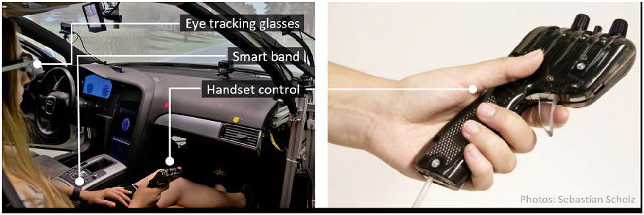
Figure 1. Driving simulator with sensor setup for discomfort assessment (left); including handset control as an experimental tool for continuous discomfort feedback during fully automated driving (right).

3.1.4 Data preparation

Data of each sensor was recorded by independent data loggers. During the study conduct, the system time of all data loggers was synchronized continuously using a software tool (Meinberg NTP Software) based on the network time protocol. After recording, raw data from all loggers were imported into a PostgreSQL-based storage and analysis framework (Beggiato, 2015). Within this framework, all sensor inputs were inspected for missing or implausible data and were then synchronized based on the driving simulator data (60 Hz). Therefore, data from all sensors were added to the corresponding timestamps of the driving simulator data. For smart band data (10 Hz), data of the last time stamp were reproduced until the next time tamp of the driving simulator data in order to adjust the different sampling rates. Gaze data provided by the eye tracker, as well as physiological data provided by the smart band, had to be further prepared to derive potential indicators of discomfort. The eye tracker recorded raw pupil diameter values for each eye. These values were preprocessed based on the procedure recommended by (Kret and Sjak-Shie 2019), including the exclusion of implausible values (<1.5mm; > 9.0 mm), dilation speed artifacts, and outliers from the trend line. Preprocessed pupil diameter values for the right and left eye were averaged to obtain a single variable for pupil dilation. The smart band provided a continuous interbeat interval by measuring the time between two consecutive heartbeats. To remove artifacts, values outside the plausible range (< 400 ms; >1,500 ms) were excluded from this variable. Based on the data provided by these sensors, additional variables were computed as potential indicators of discomfort. Supplementary Table S3 provides a full list of input variables. Eye blinks recorded by the eye tracker were transformed into a blink rate, which represents the number of blink events per second, as well as into a continuous interblink interval, which represents the time between the beginning of the last and the beginning of the next blink event. Based on the x, y, and z gaze vectors of each eye provided by the eye tracker, the standard deviation for each axis and eye was calculated for a rolling time window of 5 s. These six values were then averaged to obtain a single variable for the dispersion of gaze behavior. Based on the preprocessed interbeat intervall of the smart band, we calculated heart rate (as reciprocal of the interbeat interval), change in heart rate (hear rate slope as linear regression of heart rate) and heart rate variability (as the root mean square of successive differences between the interbeat intervals) as additional indicator variables (each over a rolling time window of 10 s). Figure 2 provides an overview of the whole data processing pipeline.

Figure 2

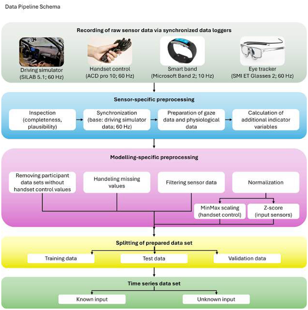
Figure 2. Overview of the data preprocessing pipeline. All sensors are shown, including eye tracking, smart band, and simulator signals, followed by preprocessing and preparation of data for time-series forecasting models.

3.2 Methodology

This section describes the problem formulation, model architecture, input/output configuration, and evaluation procedure used for discomfort prediction.

3.2.1 Model input/output definition

The TFT model is an optimized deep neural network for multi-horizon time series forecasting (Lim et al., 2021). At the core of the TFT architecture lies self-attention, a mechanism that enables the model to learn the interrelationships between sequence items in parallel. TFTs have two main characteristics that make them highly proficient in time series forecasting.

First, TFTs can support heterogeneous inputs of input data, ranging from time-dependent to static, and from known variables, which can either be obtained in advance or is already determined (such as the date or time in the future), to unknown variables, which can only be quantified at each step and are not identified in advance. Although our specific dataset does not include static features, it is important to note that, in this context, static features could represent different automated vehicles with distinct physical characteristics. It should be emphasized, however, that our analysis is conducted solely in a simulated environment, and including known variables or unknown features in the data can improve the model's performance by augmenting the input. For instance, future-known variables, such as data or signals obtained from the driving simulator at time t, are already incorporated into the forecasts. Besides, unknown inputs, like physiological signals, can also be incorporated to support the forecasting process. Thus, in time series forecasting, detailed consideration of the nature of different input features is required, with each known or unknown feature requiring specific data handling techniques to maximize the extraction of critical patterns from the data.

Second, TFTs provide an interpretability mechanism that explains the relative importance and influence of inputs. Unfortunately, the most typically used explainability methods for deep neural networks, such as Local Interpretable Model-Agnostic Explanations (LIME) (Ribeiro et al., 2016) and Shapley Additive exPlanations (SHAP) (Lundberg and Lee, 2017), are unsuitable for time series data. In their standard form, post-hoc methods like LIME and SHAP do not account for the temporal ordering of input features (Lim et al., 2021). For example, LIME builds surrogate models independently for each data point, handling each point as a separate entity without considering the time steps before or after it. Likewise, SHAP considers features independently for neighboring time steps, ignoring the dependencies between different time steps.

In order to define the input and output of a time series model, it is necessary to separate the variables into static, time-dependent, and target variables. A static covariate is represented by the variable S_i. For a time series dataset with I unique entities, such as different participants, each entity i is associated with a specific set of inputs X_{i, t} and the corresponding scalar target y_{i, t}. This separation of variables is important for building an accurate time series model. Time-dependent input features X_{i, t} are also divided into two categories $X_{i,t}=\left[z_{i,t}^T,x_{i,t}^T\right]$, where $z_{i,t}\in {\Re }^{(m_z)}$ are unknown covariate features that can only be measured at each time step and $x_{i,t}\in {\Re }^{(m_x)}$ are future known covariate features that can be predetermined, such as the velocity and acceleration of an automated vehicle. We define discomfort prediction as a sequence-to-sequence forecasting problem. Given a window of past sensor data, the model predicts a future sequence of discomfort. In this approach, we used physiological, environmental, and vehicle signals as input sequences to forecast the passenger's discomfort level up to 250 time steps ahead. We use quantile regression for our forecasting by setting the 10-th percentile at each time step. The forecasting function is defined as follows:

$\begin{array}{ll}{ŷ}_i(q,t,\tau )=f_q(\tau ,y_{i,t-k:t},z_{i,t-k:t},x_{i,t-k:t+\tau },s_i),& (1)\end{array}$

where ŷ_i(q, t, τ) is the forecasted q-th quantile for the value τ ∈ {1, ..., τ_max} in the entity i at time t, which in our scenario would be the discomfort value obtained by the handset-controller. f_q(.) is our prediction model. Simultaneously, given all past information within a finite window of retrospection k, we anticipate the target (discomfort) value for τ_max time steps ahead. In our implementation, the static information s_i is not considered, as it is evident in the dataset that every feature is time-dependent.

To match an automated driving experience in a real environment, we intentionally exclude the use of past discomfort outputs, y_{i, t−k:t}, as the input signal. This decision is based on the knowledge that discomfort cannot be directly measured in real-world scenarios. Our method, therefore, does not have autoregression, which is the process of predicting the future value of a time series given its past values. Rather, our model is based on a sequence-to-sequence framework, where the model takes a sequence of past sensor signals as input and estimates a sequence of future predictions as output. We do not give the target value (discomfort) as an input signal to the model, because it is necessary to prevent any information leakage from the target into the input sequence. By avoiding the use of auto-regression and carefully picking the input and output sequences, we can ensure that our model is accurate and robust for predicting future values of the output sequence. Multi-head attention is a strong element in TFT that allows models to focus on different parts of the input signal when making predictions. It is like having multiple sets of perspectives, and each explores a different aspect of the data, which is especially useful for capturing complex patterns from the data.

3.2.2 Temporal Fusion Transformer architecture

The TFT model also introduces Interpretable Multi-Head Attention, making it easier to understand how the model uses attention. Each attention head still focuses on different aspects of the data, but they all share and collectively decide on what is important in the data. This makes the model's decision-making process more transparent and understandable and helps us to better grasp why it makes specific predictions. The TFT model consists of five main components that improve its predictive powers:

• Gating mechanism: this component allows the network to bypass components that are not needed selectively. This helps the model handle different types of data and adapt to different scenarios.

• Variable selection network: this part of the network identifies the most important input features at each time step by ignoring less informative ones. This helps improve the model's performance, especially with real-time series data that may contain noisy or irrelevant features.

• Static covariate encoders: these encoders integrate static features into the network. It considers the context that doesn't change over time. This addition helps the model understand the impact of these static factors on the time series data.

• Temporal processing: it learns both long- and short-term temporal relationships from both known and unknown time-dependent inputs. A sequence-to-sequence layer is designed for local processing, and simultaneously, long-term dependencies are captured by an interpretable multi-head attention block.

• Prediction intervals: the model uses quantile forecasts to estimate a range of possible values for each forecast period (Wen et al., 2017). These prediction intervals provide an understanding of the uncertainty and potential variability in the predictions.

Figure 3 illustrates the structure of the TFT model. Details about these mechanisms can be found in the original publication (Lim et al., 2021). The model takes the raw temporal input signals and selects the most relevant variables at each step by using the static context and temporal dependencies. These chosen variables then go to the temporal processing component, where LSTMs capture local dependencies and multi-head attention mechanisms identify the long temporal patterns with weighting the relevance of earlier time-steps to prediction time. The gating mechanism manages information flow throughout the network, passing only the most relevant information forward to reduce noise and overfitting. Multi-head attention mechanism to improve interpretability, and is calculated as:

$\text{Attention}(Q,K,V)=\text{Softmax}\left(\frac{Q{K}^{\top }}{\sqrt{d_{\text{attn}}}}\right)V,$

where Q, K, V ∈ ℝ are the query and key and value matrices and d_attn is the attention dimension. To enhance learning capacity, multi-head attention is introduced.

$\begin{array}{l}\text{MultiHead}(Q,K,V)=\left[H_1,\dots ,H_H\right]W_H,\text{with}\\ H_h=\text{Attention}(Q{W}_Q^{(h)},K{W}_K^{(h)},V{W}_V^{(h)}),\end{array}$

where $W_Q^{(h)},W_K^{(h)},W_V^{(h)}\in ℝ$ are learned projection weights for each head h, and W_H ∈ ℝ combines the outputs concatenated from all heads. Additionally, the TFT Model originally introduced Interpretable multi-head attention ($\tilde{H}$) and shared the value projection across all heads, and is calculated as

$\tilde{H}=\frac{1}{H}{\displaystyle \sum _{h=1}^H}\text{Attention}(Q{W}_Q^{(h)},K{W}_K^{(h)},V{W}_V),$

where W_V ∈ ℝ is shared across heads. The final output is projected using W_H ∈ ℝ. This formulation allows each head to learn different temporal dependencies and makes the attention weights easier to interpret (more details in Lim et al., 2021). Finally, in the prediction intervals, probabilistic forecasts are generated, providing a range of potential outcomes and their associated uncertainties.

Figure 3

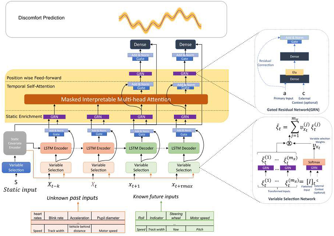
Figure 3. The proposed TFT architecture. The TFT model contains three types of inputs: static covariates, time-varying past signals (known and unknown), and time-varying future signals (known in advance). This architecture integrates key modules for interpretable and accurate forecasting. The variable selection network dynamically identifies important and relevant variables within each time window according to the static context and temporal dependencies. In addition, it combines the LSTM structure and multi-head attention mechanisms to capture local and global temporal patterns. The gating mechanism controls the flow of information and tries to reduce noise by allowing the most essential information to pass through. Notably, the interpretable multi-head attention mechanism allows the model to focus on specific time steps or patterns in the past that are most relevant to the current prediction, which is helpful to capture long-range temporal dependencies that LSTM layers alone may miss, and improves both performance and interpretability in sequences where causes and effects are temporally distant.

We used the TFT architecture as described by (Lim et al. 2021) without structural modifications.

3.2.3 Evaluation metrics

To assess and compare the forecasting performance, four statistical metrics are utilized: Mean Absolute Error (MAE), Root Mean Square Error (RMSE), Coefficient of determination (R²), and Pearson correlation (P_corr). These metrics provide quantitative measures of the accuracy and quality of the forecasts. For a target sequence y = {y₁, y₂, …, y_n} and a predicted sequence ŷ = {ŷ₁, ŷ₂, …, ŷ_n}, the formulas for these metrics are as follows:

$\begin{array}{ll}\text{MAE}=\frac{1}{n}{\displaystyle \sum _{t=1}^n}||y_t-{ŷ}_t||& (2)\end{array}$

$\begin{array}{ll}\text{RMSE}=\sqrt{\frac{1}{n}{\displaystyle \sum _{t=1}^n}{(y_t-{ŷ}_t)}^2}& (3)\end{array}$

$\begin{array}{ll}{R}^2=1-\frac{{\displaystyle {\sum }_{t=1}^n}{(y_t-{ŷ}_t)}^2}{{\displaystyle {\sum }_{t=1}^n}{(y_t-E_t\left[y\right])}^2}& (4)\end{array}$

$\begin{array}{ll}{P}_{\text{corr}}=\frac{\text{C}\text{o}\text{v}(y,ŷ)}{\text{s}\text{t}\text{d}(y)\text{s}\text{t}\text{d}(ŷ)}& (5)\end{array}$

The MAE and RMSE metrics are utilized to evaluate the error level between the predicted and actual results. Lower values of these metrics indicate higher forecasting performance. The coefficient of determination R² compares the variance of the residual error to the variance of the target sequence around its temporal average E_t[y]. The particular benefit of R² is that it provides a normalized measure of how well the predictions explain the variability of the actual data. A coefficient of determination equal to 1 denotes that the predictions perfectly fit the data. The P_corr, calculated using the covariance Cov() and standard deviation std() functions, represents the strength of the linear relationship between the target and predicted signals, ranging from –1 to 1. An absolute value of 1 indicates a perfect relationship between the target and the predicted signal. It is mainly useful for assessing the linear relationship between the target values and the predicted signal. TFT training involves a joint minimization of the quantile loss, as described in (Wen et al. 2017), which is aggregated across all quantile outputs. To achieve quantile predictions, the Quantile Loss (QL) is explicitly formulated for each quantile q as follows:

$\begin{array}{ll}L(\text{Ω},W)={\displaystyle \sum _{y_t\in \text{Ω}}}{\displaystyle \sum _{q\in Q}}{\displaystyle \sum _{\tau =1}^{{\tau }_{max}}}\frac{QL(y_t,ŷ(q,t-\tau ,\tau ),q)}{M{\tau }_{max}}& (6)\end{array}$

$\begin{array}{ll}\text{QL}(y,ŷ,q)=q·\text{max}\left\{0,(y-ŷ)\right\}+(1-q)·\text{max}\left\{0,(ŷ-y)\right\}& (7)\end{array}$

Ω denotes the training data domain, which comprises M samples, W stands for the weights associated with TFT, and q is a set of quantile values. The set q comprises the following quantiles:

$\begin{array}{ll}q=\left\{0.1,0.27,0.36,0.45,0.54,0.63,0.72,0.81,0.9\right\}& (8)\end{array}$

The size of the set is 10, indicating that 10 quantile values are being considered.

3.2.4 DeepAR

DeepAR is an autoregressive recurrent network that can learn a single global model from the past data of all time series in a dataset (Salinas et al., 2020). Compared to traditional statistical methods like ARIMA (Newbold, 1983), DeepAR obtains a better performance and can be trained much faster than TFT, making it a practical option for the discomfort prediction task. DeepAR utilizes an encoder-decoder architecture based on LSTM, as indicated in Figure 4. The encoder takes past time series data and processes it through a stack of LSTMs to generate a compressed representation of the state of the time series. The decoder then takes this representation as input and generates a probability distribution over the future values of the time series. During training, DeepAR is optimized to minimize the negative log-likelihood of the actual future values given the predicted probability distribution. This allows it to capture the uncertainty and variability in the time series, making it an effective tool for generating accurate probabilistic forecasts. In our setup, we used a one-layer LSTM encoder-decoder architecture and the normal distribution for the output.

Figure 4

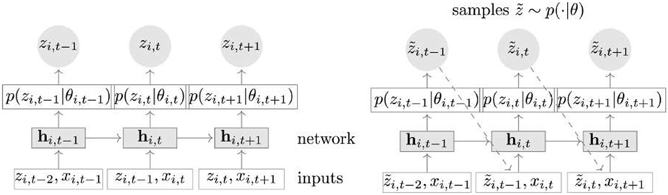
Figure 4. DeepAR model overview. Training phase (left side): At time step t, the model gets three inputs: the covariates x_{i, t}, the target value at the previous time step, z_{i, t−1}, and the last output from the model, h_{i, t−1}. The network's output at time t, denoted as h_{i, t} = h(h_{i, t−1}, z_{i, t−1}, x_{i, t}, Φ), is utilized to calculate the parameters θ_{i, t} = θ(h_{i, t}, Φ) for the likelihood function (z|θ), which in turn is employed to train the model parameters. During the prediction phase, the historical data of the time series z_{i, t} is given for t<t₀. For the prediction interval (right side) when t≥t₀, a predicted sample ẑ_{i, t} (.|θ_{i, t}) is generated, fed back into the model for forecasting the subsequent point, and this process is continued until the end of the forecast period at t = t₀+T, producing a single sample path. By repeating the prediction procedure, multiple sample paths are generated, illustrating the combined predicted distribution (Salinas et al., 2020; Graves, 2013).

4 Performance evaluation

4.1 Preprocessing

Because of the possible shortcomings of the sensors, the generation of our dataset was highly susceptible to missing entries, inconsistent collection, and noise due to the simultaneous use of different sensors. These faulty readings and the occasional absence of values may provide an incorrect view of the overall domain from which the data is supposedly sampled. Furthermore, we eliminated nine participants from our dataset because they had no discomfort reaction throughout the experiment. Eleven participants were further excluded as their gaze data had no entries. The remaining 80 participants are included in the dataset. Data normalization is a transformation performed on a single input to evenly distribute and scale the data to a range acceptable to the network. To establish a standard baseline, input features are rescaled through standardization or Z-score normalization before being fed into the TFT and DeepAR models (Equation 9).

$\begin{array}{ll}z=\frac{x-\text{mean}(x)}{\text{std}(x)}& (9)\end{array}$

The MinMaxScaler method from scikit-learn (Pedregosa et al., 2011) is used to normalize the handset-controller values between 0 and 1. This normalization process is applied only once to the input data before it is used in the models. There are no multiple sets generated randomly for normalization. Finally, all datasets are partitioned into training, validation, and test sets with a ratio of 70% (56 participants): 10% (eight participants): 20 % (16 participants).

The discomfort experienced by each participant during the test drive was distinct and varied. A detailed overview of the handset control responses of participants during the test drive is illustrated in Figure 5. It is visible that different participants displayed different response patterns. For instance, Participant Number 5 showed relatively trivial reactions, mostly during complex traffic scenarios. Conversely, participants 38 and 40 demonstrated their most noticeable reactions outside complex traffic scenarios, as indicated by the gray shade segments in the graph. Nevertheless, many reactions must occur outside of these traffic scenarios. These additional responses add complexity to predicting and analyzing the discomfort experienced during the test drive.

Figure 5

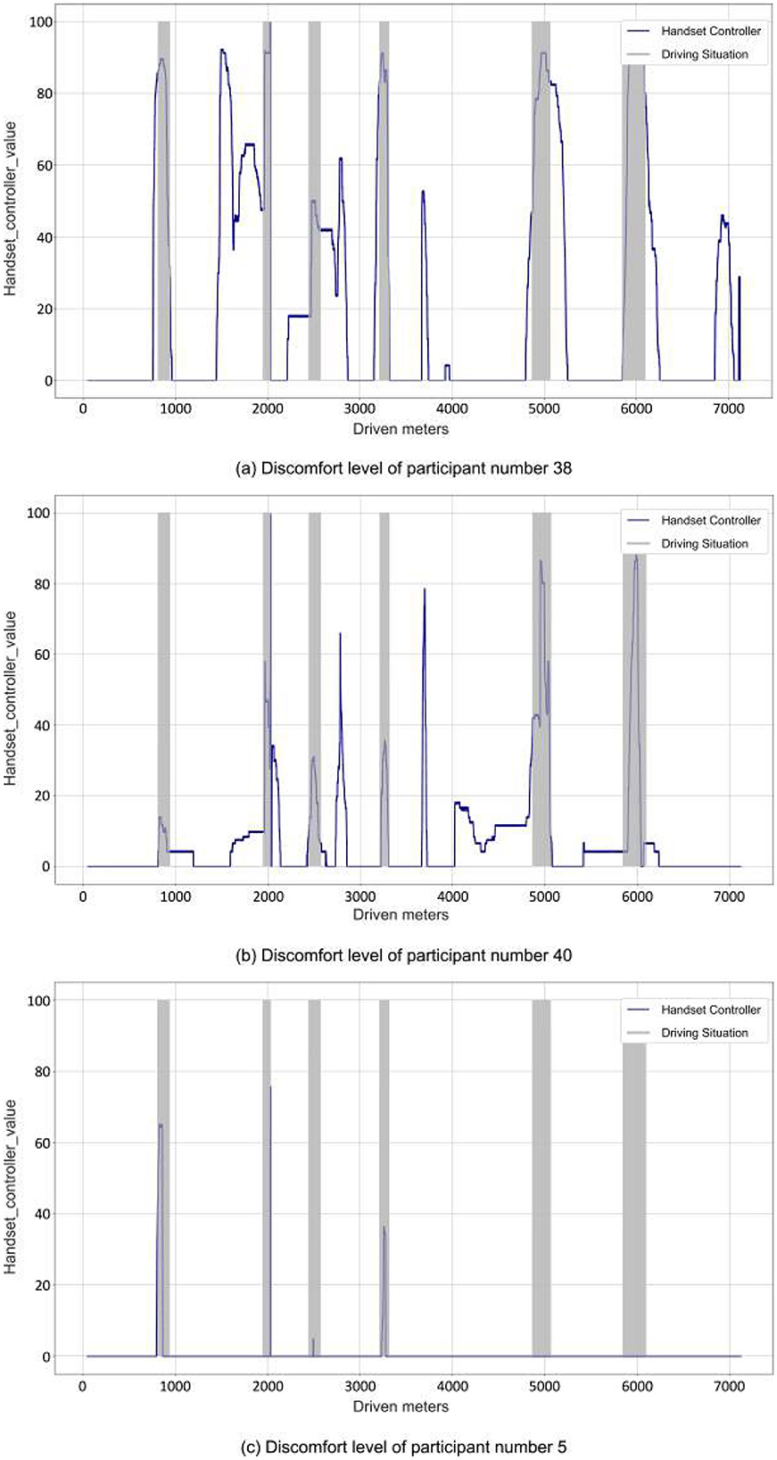
Figure 5. Handset controller values (discomfort levels) of three random participants. (a–c) Correspond to these different random participants and illustrate their levels of discomfort in an identical scenario. The gray-shaded area represents complex and, therefore, potentially discomfort-inducing driving conditions, such as traffic lights or lane changes.

The overall data pipeline, from data preparation to preprocessing, is illustrated in Figure 2.

4.2 Training procedure

In this study, we use the PyTorch-Forecasting library for implementing our model (Beitner, 2020). This library has a specific class, TimeSeriesDataset, to organize and structure our data in a format suitable for training the model. Our analysis involves the use of two distinct models: TFT-full and TFT-restricted. In the TFT-full model, all physiological signals such as pupil diameter and blink rate variables are considered as unknown inputs. However, the state of the vehicle (e.g., speed, acceleration) and characteristics of the driving environment (e.g., speed and distance to surrounding vehicles) are treated as known inputs. This approach is based on our assumption that the automated vehicle possesses inherent knowledge about its planned actions and obtains information about the surrounding environment. We consider these inputs to be known and expect an improvement in the accuracy of passenger discomfort prediction. In the TFT-restricted model, we consider both the environmental and physiological signals as unknown inputs while keeping the vehicle signals as known inputs. This method was used to explore the relationship between the known signals from the driving simulator and the level of discomfort experienced by passengers. Figure 6 shows the differences between the inputs of the TFT-restricted and TFT-full models. For example, let's consider a situation where the vehicle is approaching an intersection. In the TFT-full model, the vehicle has information about its current speed, acceleration, and distance to the intersection (these are the known inputs). These known inputs are based on the vehicle's sensors and programmed route. The vehicle is aware that it will need to slow down or stop at the intersection, as this knowledge is part of its programmed actions. However, passenger reactions, like changes in pupil size or blinking rates as they approach the intersection, are considered unknown inputs because they vary from participant to participant and cannot be predicted accurately in advance. In the TFT-restricted model, the vehicle is still aware of its current speed and acceleration (known inputs). Nevertheless, other environmental signals, such as the behavior of surrounding vehicles, are considered as unknown inputs, as they may change unexpectedly. Similarly, the physiological reaction of the passengers remains unknown. In addition, we train a DeepAR model for comparative analysis. However, due to the DeepAR model's autoregressive nature, the handset controller's value is treated as an unknown input. Unlike the TFT model, where the handset-controller value was explicitly excluded as an input, the DeepAR model directly incorporates this value as an input variable. The decision to omit the past discomfort signal when training the TFT was made based on the understanding that any sensor in a real-world scenario cannot directly measure discomfort. However, DeepAR is not designed to predict a variable whose past is not provided; therefore, it was necessary to use the past discomfort signal in an autoregressive manner when training this model.

Figure 6

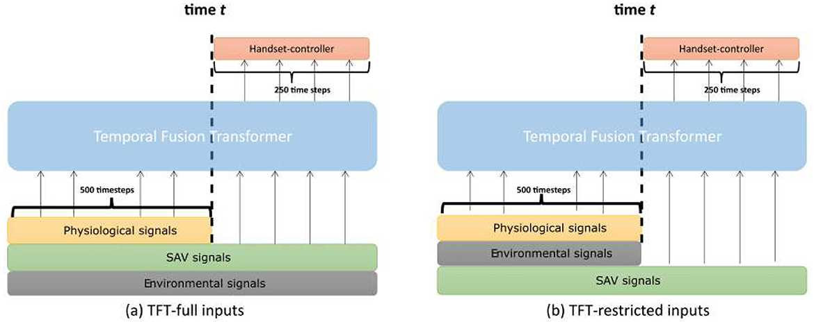
Figure 6. Input differences between TFT-full (a) and TFT-restricted models (b) for a prediction window of 250 steps, with 500 past time steps of inputs.

4.3 Hyperparameter optimization

The hyperparameters of both models are optimized through a random search, which involves 15 iterations. This optimization process is performed on the training data. During each iteration, a different set of hyperparameters is randomly selected and evaluated. The performance of each set is assessed based on its ability to predict passenger discomfort accurately. The best-performing hyperparameters are then chosen for the final models. The search ranges for all hyperparameters are listed in a Supplementary Table S1. To reduce the dimension of hyperparameter search and the amount of guesswork involved in selecting a good starting learning rate, we use the learning rate finder (Smith, 2017) with the use of Pytorch Lightning. The TFT models reported here are trained using the final hyperparameters of Supplementary Table S2.

5 Results

5.1 Time series prediction

We first investigate the impact of different input window sizes on the performance of the TFT-full, TFT-restricted, and DeepAR models. The input window sizes are 500 (approximately 8 s), 400 (about 6.5 s), 300 (about 5 s), and 200 (about 3.5 s) time steps. The objective is to determine the optimal window size of the input signal for detecting discomfort using both the full TFT model and the restricted version. Previous experiments with non-transformer-based neural networks indicated poor results for small window sizes, such as less than 1 second. As a result, the search space for window sizes is constrained to these sizes to focus on potential improvements in model performance. Predictions are made for a horizon of 250 time steps (about 4 s) ahead.

Each model is trained 10 times with randomly initialized weights to avoid any possible bias. Table 1 shows the mean and standard deviation of the evaluation metrics over the 10 different training runs for the TFT-full, TFT-restricted, and DeepAR models. By presenting the mean and standard deviation, we provide a measure of the average performance of the model as well as the variability of the results across different training runs.

Table 1

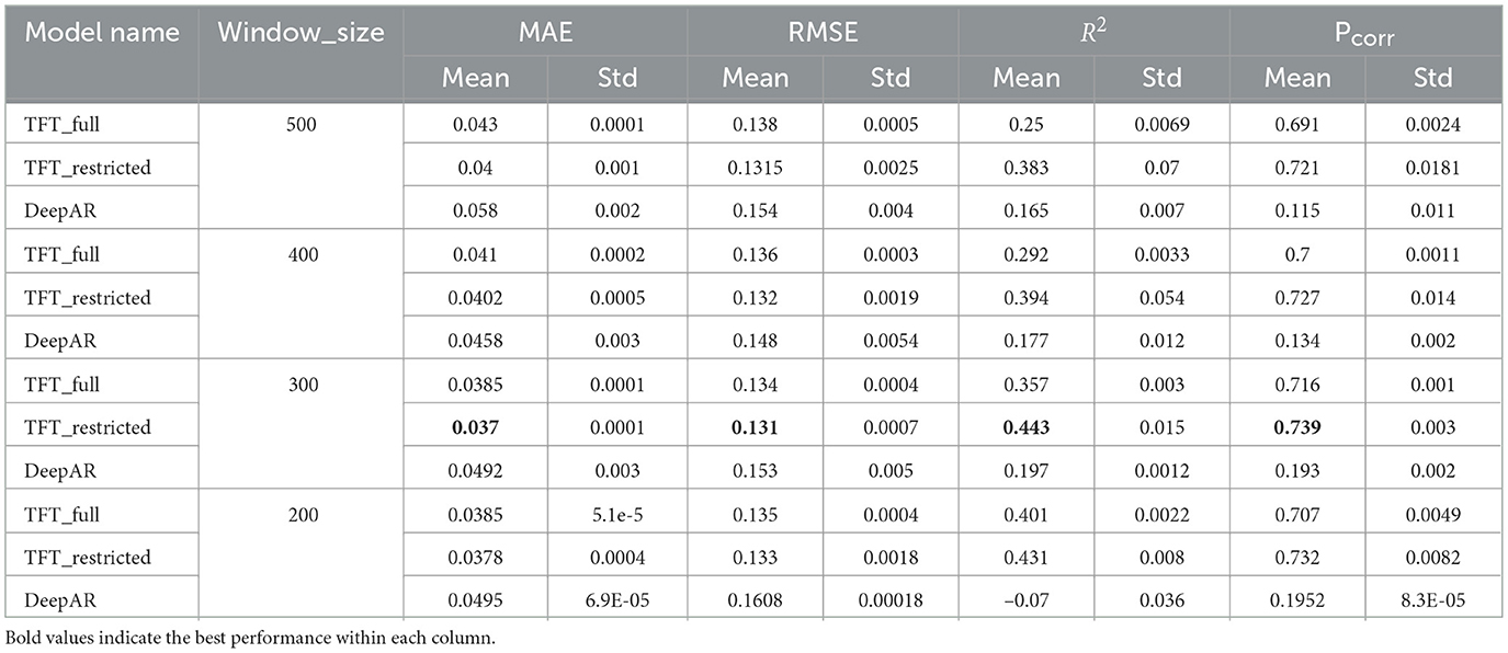
Table 1. Comparative analysis of model performance in a 250-step prediction on the test set using different input window sizes. The data of each sensor was synchronized based on the 60 Hz of the driving simulator data.

According to the data in Table 1, it is clear that the TFT-restricted model, with a window size of 300, outperformed the other models. To evaluate the statistical significance of these performance differences, we performed paired t-tests between the TFT-restricted and the other models across 10 independent runs. Table 2 reports the mean and 95% confidence intervals (CI) of the TFT-restricted model along with the p-values from these comparisons. The results demonstrate that the improvements of TFT-restricted over both TFT-full and DeepAR are statistically significant (p < 0.05) across all metrics and window sizes.

Table 2

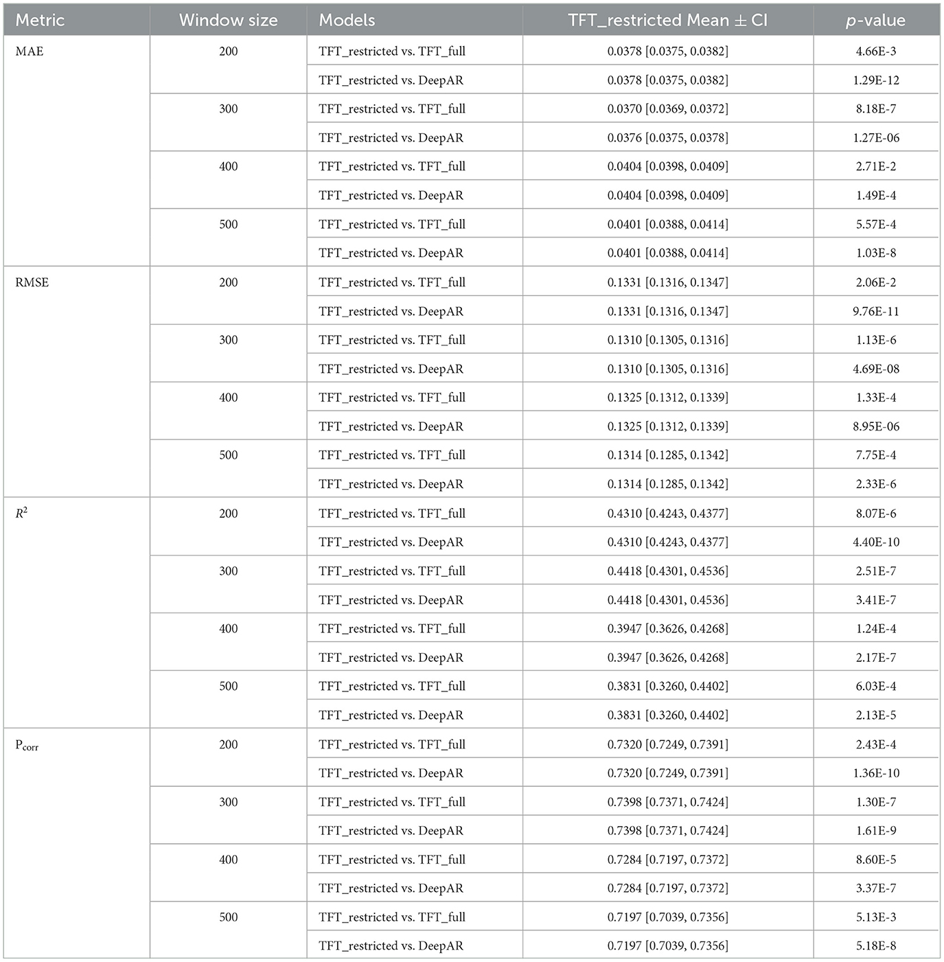
Table 2. Performance comparison of TFT-restricted against other models for all input window sizes. We considered the mean and 95% confidence intervals (CI) for 10 runs. Paired t-tests were applied to evaluate statistical significance (p = 0.05).

Supplementary Table S4 presents the Diebold-Mariano (DM) (Diebold and Mariano, 2002) test to again statistically evaluate the performance of the proposed TFT and DeepAR models as secondary analysis.

Figure 7 depicts the analysis of MAE performance for our different models across various window sizes. The results indicate that a window size of 300 performs better, highlighting its suitability as the optimal window size for our model. A shorter window size allows our model to focus on fewer time steps. Across various window sizes, the TFT-restricted model consistently outperforms the other models. Taking a closer look at the predictions, we can see in Figure 8 the predictions made by the restricted model for a single sequence of a random participant. For this specific participant with a fixed horizon, given different sizes of past windows, the prediction is shown, i.e., the prediction window in all the subplots is the same. These plots represent the handset controller and the predicted values using the last 300, 400, and 500 time steps as input. The predicted value is plotted with the prediction intervals, and the orange area shows the uncertainty of the predicted values. Figure 8a highlights the individual prediction for 250-time steps ahead using the TFT-restricted model with a window size of 300, which closely aligns with the ground truth. Conversely, Figures 8b, c demonstrate a decrease in prediction accuracy and certainty as the window size increases. Furthermore, a larger window size diminishes the model's sensitivity to short-term data variations, resulting in reduced accuracy for short-term predictions. In general, using quantiles to compute uncertainty in time series forecasting allows the model to better understand the potential range of outcomes.

Figure 7

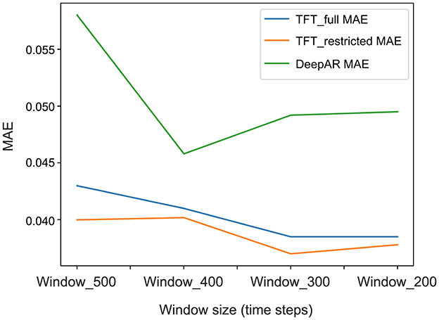
Figure 7. Comparison of MAE values of TFT-full, TFT-restricted, and DeepAR for various input window sizes.

Figure 8

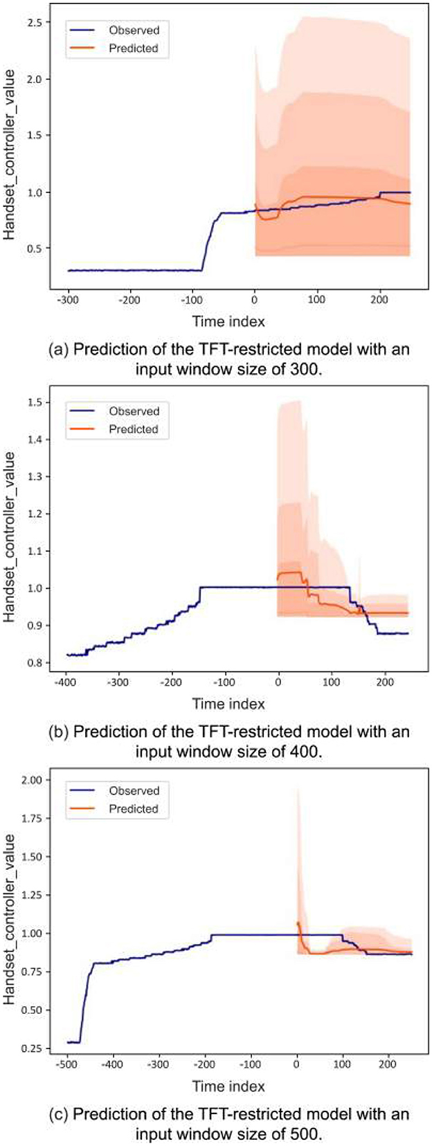
Figure 8. Visual representation of predictions from the TFT-restricted for a single sequence with different input window sizes. The sequence was randomly selected from the test set and demonstrated the model's performance on individual instances. The orange line indicates the model's predictions, while the blue line corresponds to a specific participant's ground truth handset controller values. The orange-shaded area represents the prediction intervals, providing insights into the uncertainty in the forecast. The transparency in the orange area indicates the confidence level. The uncertainty is computed using quantiles. (a–c) Correspond to the prediction window sizes of 300, 400, and 500, respectively.

Figure 9 illustrates the one-step-ahead predictions of discomfort for the participant's entire route from the test set. To maintain fairness in the comparison, we specifically visualize the TFT-restricted, TFT-full, and DeepAR models, all with a window size of 300, as it has exhibited superior performance across various evaluation metrics. Among these models, the TFT-restricted model shows the closest alignment with the ground truth and achieves an R² score of 0.62. On the other hand, the TFT-full model demonstrates a reasonably close alignment with an R²-score of 0.59. Finally, the DeepAR model shows the poorest result, with an R²-score of 0.4. Figure 10 shows the TFT-restricted model's prediction uncertainty for a test participant. We use a 300-time step window size (equivalent to 5 s). Our analysis focuses on the one-step-ahead prediction and employs a set of 10 quantiles chosen as our quantile levels. Following this, we compute these quantiles' mean and standard deviation and visualize the uncertainty by displaying both the mean and standard deviation across the entire trajectory. This helps us to understand the uncertainty dynamics within the TFT predictions for the entire test route. It is observable that when discomfort increases slowly, the uncertainty associated with TFT predictions tends to be lower compared to situations where discomfort increases rapidly. This can be attributed to the temporal nature of the TFT model and its window size of 300 time steps. The model captures and leverages temporal patterns in the data, enabling it to make predictions based on historical information within the defined window. On the other hand, when discomfort increases rapidly, the patterns and dynamics change abruptly within the defined window. The TFT-restricted model may struggle to capture and interpret such rapid changes effectively, leading to higher uncertainty in its predictions. Another interesting relationship is the correlation between the uncertainty level of the model and the rate of change in the state of discomfort. This relation will show whether the higher uncertainty arises mostly when the rate of discomfort is significantly above zero, when only the absolute values are considered. The rate of change in discomfort is the derivative of the discomfort signal, which can be obtained by the absolute difference in discomfort at time t minus discomfort at time t−1, divided by Δt. Therefore, one can plot the derivative of the discomfort signal against the standard deviation of the prediction. The analysis, encompassing the entire test set, showed a P_corr of 0.474. This visualization is included in Supplementary Figure S1.

Figure 9

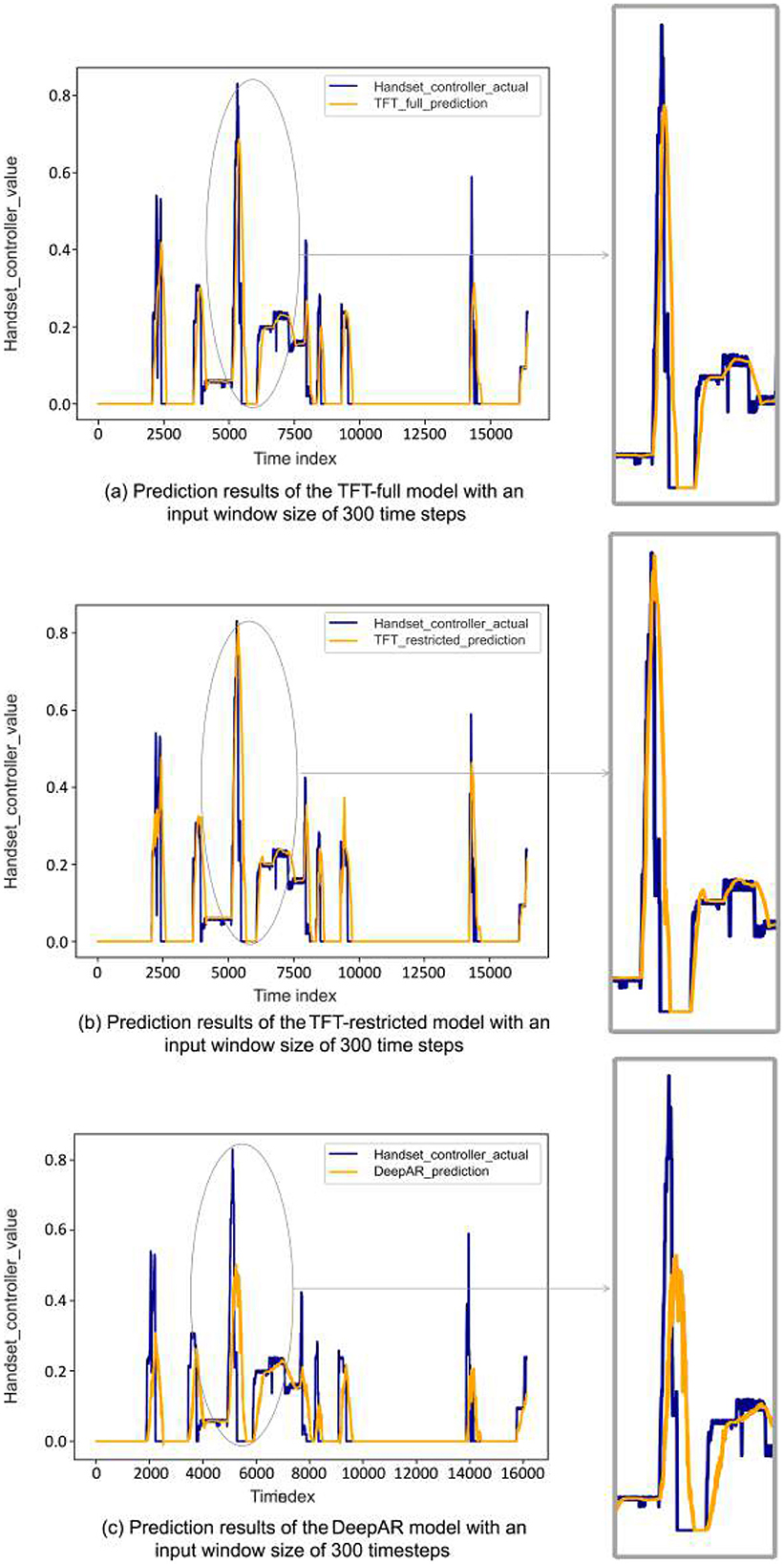
Figure 9. Visualization of one-step-ahead discomfort predictions across a participant's entire route from the test set. The focus is on TFT-full (a), TFT-restricted (b), and DeepAR models (c); all have the configuration of the input window size of 300. The zoomed area on critical points demonstrates the details of the predictions.

Figure 10

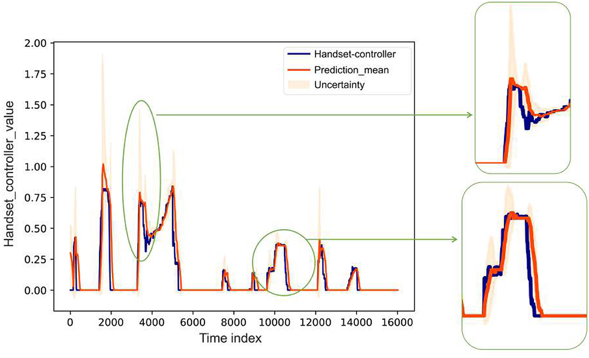
Figure 10. Visualization of the uncertainty in TFT-restricted model predictions for a test participant using 300 time steps. Our analysis highlights the one-step-ahead prediction, using 10 quantiles from 10 training iterations. The mean and standard deviation for these quantiles are computed, providing a comprehensive visualization of uncertainty across the entire trajectory averaged over 10 training iterations with different starting conditions.

5.2 Interpretability

In this section, we show how the restricted TFT model with a window size of 300 helps to interpret the relationship between the input signals (known and unknown). We demonstrate the model's interpretability by assessing the importance of each input signal in the prediction process. Additionally, we showcase the visualization of attention-weighting patterns. Variable importance is quantified by analyzing the variable selection weights. In concrete terms, we aggregate the selection weights for each variable across our entire test set and plot the 10-th percentile of each sampling distribution. The results are shown in Figure 11, which shows the importance of input signals observed in the past, Figure 12, which plots the importance of input signals known in the future, and Figure 13, which predicts the attention weighting patterns. No variable importance was assigned to static inputs as they were not considered in the dataset. The encoder variables, representing known past values at prediction time, consist of previously selected features and a relative time index. Figure 11 displays the importance of each variable known at prediction time. Acceleration received the highest attention importance with a proportion of 22%, followed by the speed of the rear car (11.5%) and the average standard deviation of the gaze vector (10.33%). Variables on the encoder side with gradually decreasing importance are the roll, vehicle indicators, heart rate changes, and other signals depicted in Figure 11. The variables in the decoder include the signals that are known until the end of the prediction time steps. Their interpretation and significance are shown in Figure 12. Based on the decoder chart, it is clear that the roll signal of the vehicle shows the highest attention importance, accounting for nearly 17.9% of its impact on predicting the discomfort sequence. This is followed by the indicator of the vehicle (14.2%) and the angle of the steering wheel (11.5%). The RPM of the vehicle had the lowest attention importance, with a score of only 5%. Figure 13 illustrates the attention-weighting patterns across all our test datasets. In this graph, we specifically represent the 10th percentile of each sampling distribution, which provides insight into the lower range of attention weights. The observed data exhibits a U-shaped pattern, signifying that the model places significant importance on both the initial and final portions of the input sequence. This pattern suggests that the information at the beginning and end of the period is crucial for the model's predictions.

Figure 11

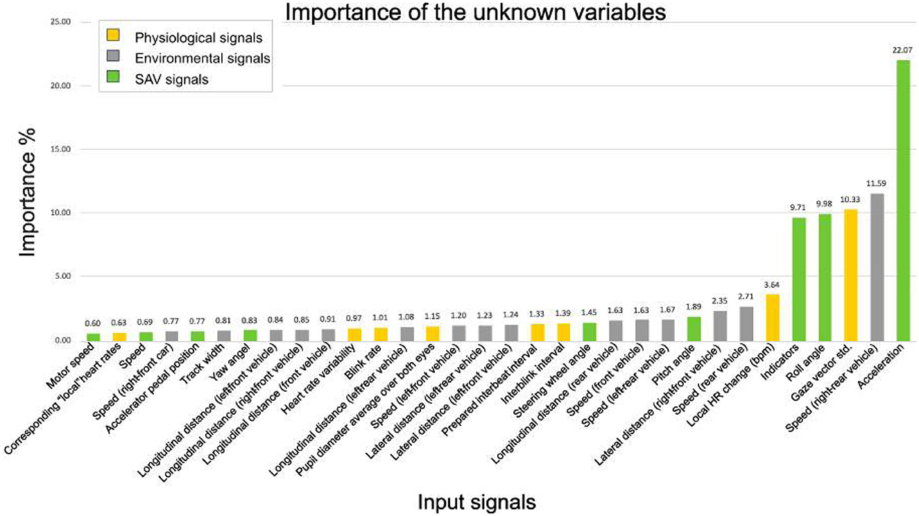
Figure 11. Visualizing the importance analysis of encoder variables (or unknown input signals) in TFT-restricted with 300 time steps. The analysis is conducted across the entire test set and averaged over 10 training runs of the model. We classify the unknown signal using different colors, according to the definition of TFT restricted in Figure 6b. The analysis provides an understanding of the importance of each unknown variable over time.

Figure 12

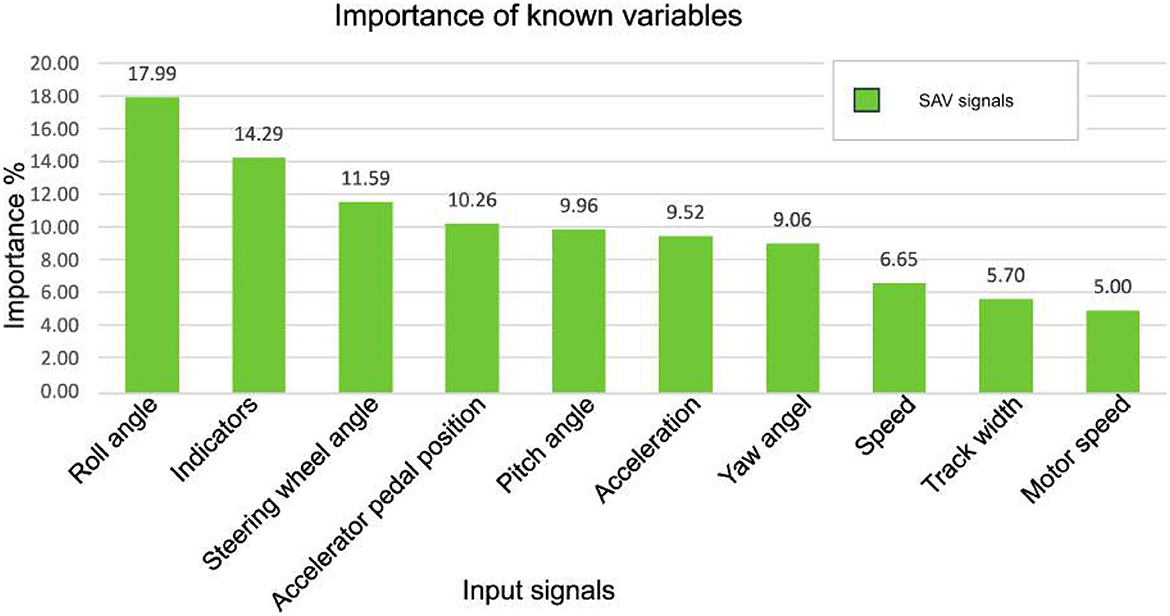
Figure 12. Exploring the importance analysis of decoder variables (or known input signals) in TFT-Restricted with 300-time steps. The analysis is operated across the entire test set and averaged over 10 training runs of the model. The analysis provides an understanding of the importance of each known variable over time.

Figure 13

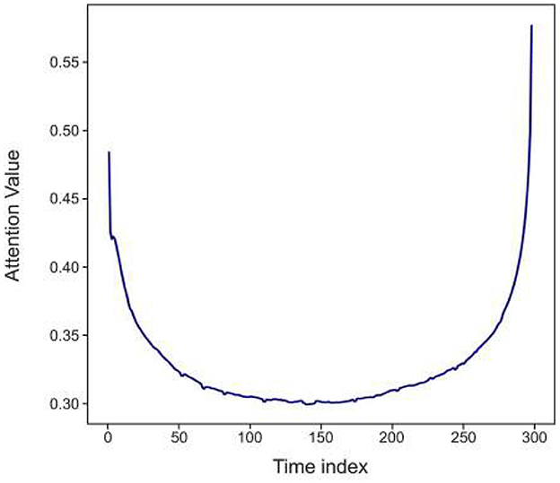
Figure 13. Visualizing attention weight patterns in TFT-Restricted with a 300-time step input window size. This visualization contains the entire test set, highlighting the importance of both the beginning and end of the input sequence.

6 Discussion

Assessing discomfort in automated vehicles is challenging due to multiple factors like inter-individual differences between humans, diverse scenarios, and unpredictable environmental conditions. In this study, we trained two temporal Transformer-based models, TFT-full and TFT-restricted, to detect discomfort during automated driving. TFT models generally have interesting properties for time series forecasting, such as interpretability, handling of long-term dependencies, relevant input feature selection, data redundancy reduction, and versatility for different datasets. Furthermore, TFT models are well-suited for real-world scenarios, including the detection of discomfort in automated vehicles. These features enable us to make accurate predictions and surpass sophisticated methods like DeepAR. The analysis of the importance of decoder and encoder variables highlighted the significance of combining different input sources. The six most important input variables (see Figure 11) included all four groups of input data used in this study (gaze behavior, physiological parameters, driving environment, and driving behavior of the automated vehicle). This emphasizes the strength of a multimodal discomfort assessment compared to single-mode approaches, which corresponds with previous studies in this context (e.g., Niermann et al., 2021). Probable reasons for this finding are that (a) human gaze parameters and physiological parameters can be expressions of diverse psychological states (unspecificity) and (b) identical environmental factors (e.g., driving environment, driving behavior of the automated vehicle) can evoke different psychological and physiological reactions for different individuals (interindividual differences). Therefore, detecting psychological states such as discomfort in automated driving benefits from interpreting multiple signals from different sources in combination with each other, e.g., using context information about the driving environment and driving behavior of an automated vehicle to interpret the gaze behavior and physiological parameters of its passengers. Furthermore, it becomes crucial in future investigations to investigate the importance of adjusting the past window size in relation to the future window size. Our experiments explore varying past window sizes of 500, 400, 300, and 200 to predict a constant 250 time steps (about 4 s), and the optimal performance belongs to the TFT model with a window size of 300 (about 5 s). This emphasizes the importance of studying different prediction window sizes in future studies by finding a trade-off between the length of the past and prediction windows.

To simulate real-world conditions where actual discomfort values are not available during driving, we intentionally excluded past discomfort levels from the model inputs. This is a strength of the model and avoids data leakage. Regarding interpretability, our main focus was to understand the importance of the input signal types (e.g., sensor or feature names) rather than identifying which specific parts of the time series were important for the predictions. Therefore, we focused on feature-level interpretability using variable importance scores. The presented bar plots of variable importance (Figures 11, 12) summarize the TFT's multi-head attention weights aggregated over the test set and prediction window. This shows the attention distribution across input variables and shows interpretable insights into which features contributed most to the discomfort predictions. In addition, Figure 13 shows aggregated attention weights over the input sequences. Future work could explore visualizing attention heatmaps over individual prediction windows to provide even deeper temporal interpretability. We performed a participant-based data split. Specifically, participants in the test set were not present in the training or validation sets; therefore, the model's performance reflects its ability to generalize to unseen samples.

When interpreting the study results, a few methodological limitations must be considered. First, the simulated driving environment provides lower external validity than real-world driving. Since failures of the automated driving system would have had no actual safety effects, the participants might have felt safer and more comfortable during fully automated driving in the driving simulator than they would have felt in real-world traffic. Therefore, discomfort values could be underestimated by our results. However, driving simulations currently represent the only approach to provide the experience of fully automated driving (SAE-Level 5) (J3016-201806, 2024) along realistic routes (i.e., long, diverse routes with a lot of other road users) in a safe and ethical manner. Therefore, the results of the study should be evaluated in real, fully automated vehicles in the future. Second, the group of participants was not representative of the population. Since taking part in the study was voluntary, it was subject to some degree of self-selection. Therefore, the participants could have been more interested in technology or more open toward driving automation then the average of the population, which might also have led to lower levels of discomfort experienced during automated driving. In addition, the age and gender distribution of the sample implicates an overrepresentation of younger women, which might restrict the generalizability of the results to other age groups and genders. Especially elderly drivers (i.e., 65 years and older) are known to report specific attitudes and experiences regarding modern technologies such as fully automated driving (see, e.g., Hartwich et al., 2018). Therefore, further studies based on more heterogeneous participant groups are desirable. In the end, the TFT model, like many sophisticated deep learning models, faces limitations in terms of training time, especially on large datasets. The computational complexity associated with transformer-based architectures can result in longer training durations. Future investigations should explore techniques such as model compression or quantization to improve scalability and efficiency for real-time applications in automated vehicles. Finally, we acknowledge that predictive uncertainty is an inherent aspect of such forecasting models. As shown in Figure 8, variations in input-window size affect model performance, and the length of temporal context can influence both predictive accuracy and stability. Additionally, Supplementary Figure S1 shows that the standard deviation of predictions changes with the rate of change in discomfort. These observations show that predictive uncertainty may arise from both the selection of temporal context in input and the prediction window size, which could be another aspect of investigation in future work, to model and quantify such uncertainty explicitly.

7 Conclusion

In our study, TFT-restricted outperformed TFT-full and the autoregressive model DeepAR in discomfort prediction, delivering superior results for all metrics. We speculate that TFT-restricted outperformed TFT-full may be due to its statements of environmental signals as unknown inputs, which allows the model to learn more from the vehicle's signals and make better predictions. Finally, our study shows that the TFT can capture temporal dependencies in the data and help us interpret the model for detecting discomfort. This is essential for analyzing and improving people's acceptance of using automated vehicles. However, our study focused on adapting the TFT model to predict discomfort in a simulated environment; we did not explore domain adaptation, transfer learning, or robustness aspects such as missing data or sensor failures in a real-world application. These topics are outside the scope of the current investigation, but we recognize them as important directions for future research.

Data availability statement

The data analyzed in this study is subject to the following licenses/restrictions. The dataset used in this study was collected as part of the Ko-MTI project and is described in detail in its final report. The raw data supporting the conclusions of this article are available upon request from the author (Franziska Hartwich). Requests to access these datasets should be directed to ZnJhbnppc2thLmhhcnR3aWNoQGl3dS5mcmF1bmhvZmVyLmRl.

Ethics statement

Ethical approval was not required for the study involving humans in accordance with the local legislation and institutional requirements. The study only contributed the data analysis based on an existing dataset, see (Bocklisch et al., 2023, for details). No new data collection was conducted as part of this study. Written informed consent to participate in this study was not required from the participants or the participants' legal guardians/next of kin in accordance with the national legislation and the institutional requirements.

Author contributions

MA: Formal analysis, Investigation, Methodology, Visualization, Writing – original draft, Writing – review & editing. FH: Data curation, Formal analysis, Validation, Writing – original draft, Writing – review & editing. JV: Validation, Supervision, Writing – review & editing. FB: Data curation, Funding acquisition, Resources, Supervision, Writing – review & editing. FHH: Funding acquisition, Writing – review & editing, Resources, Supervision.

Funding

The author(s) declare that financial support was received for the research and/or publication of this article. This research was funded by the German Federal Ministry of Education and Research (Bundesministerium für Bildung und Forschung), grant number 16SV8297.

Conflict of interest

JV was employed at eOdyn.

The remaining authors declare that the research was conducted in the absence of any commercial or financial relationships that could be construed as a potential conflict of interest.

Generative AI statement

The author(s) declare that no Gen AI was used in the creation of this manuscript.

Any alternative text (alt text) provided alongside figures in this article has been generated by Frontiers with the support of artificial intelligence and reasonable efforts have been made to ensure accuracy, including review by the authors wherever possible. If you identify any issues, please contact us.

Publisher's note

All claims expressed in this article are solely those of the authors and do not necessarily represent those of their affiliated organizations, or those of the publisher, the editors and the reviewers. Any product that may be evaluated in this article, or claim that may be made by its manufacturer, is not guaranteed or endorsed by the publisher.

Supplementary material

The Supplementary Material for this article can be found online at: https://www.frontiersin.org/articles/10.3389/fcomp.2025.1639505/full#supplementary-material

References

Beggiato, M., Hartwich, F., and Krems, J. (2019). Physiological correlates of discomfort in automated driving. Transp. Res. F Traffic Psychol. Behav. 66, 445–458. doi: 10.1016/j.trf.2019.09.018

Crossref Full Text | Google Scholar

Beggiato, M. M. (2015). Changes in Motivational and Higher Level Cognitive Processes When Interacting With in-vehicle Automation. PhD thesis, Technische Universität Chemnitz. Available online at: https://nbn-resolving.org/urn:nbn:de:bsz:ch1-qucosa-167333

Google Scholar

Beitner, J. (2020). Pytorch-forecasting: A Library for Time Series Forecasting with Pytorch.

Google Scholar

Bocklisch, F., Hartwich, F., Kreißig, I., Rozsa, F., Assarzadeh, R., Vitay, J., et al. (2023). Ko-mti Project Final Report. Chemnitz.

Google Scholar

Constantin, D., Nagi, M., and Mazilescu, C.-A. (2014). Elements of discomfort in vehicles. Procedia-Soc. Behav. Sci. 143, 1120–1125. doi: 10.1016/j.sbspro.2014.07.564

Crossref Full Text | Google Scholar

Dettmann, A., Hartwich, F., Roßner, P., Beggiato, M., Felbel, K., Krems, J., et al. (2021). Comfort or not? Automated driving style and user characteristics causing human discomfort in automated driving. Int. J. Hum. Comput. Interact. 37, 331–339. doi: 10.1080/10447318.2020.1860518

Crossref Full Text | Google Scholar

Diebold, F. X., and Mariano, R. S. (2002). Comparing predictive accuracy. J. Bus. Econ. Stat. 20, 134–144. doi: 10.1198/073500102753410444

PubMed Abstract | Crossref Full Text | Google Scholar

Dommel, P., Pichler, A., and Beggiato, M. (2021). “Comparison of a logistic and SVM model to detect discomfort in automated driving,” in International Conference on Intelligent Human Systems Integration (Cham: Springer), 44–49. doi: 10.1007/978-3-030-68017-6_7

Crossref Full Text | Google Scholar

Gehring, J., Auli, M., Grangier, D., Yarats, D., and Dauphin, Y. N. (2017). “Convolutional sequence to sequence learning,” in International Conference on Machine Learning (Sydney, NSW: PMLR), 1243–1252.

Google Scholar

Graves, A. (2013). Generating sequences with recurrent neural networks. arXiv [preprint]. arXiv:1308.0850. doi: 10.48550/arXiv.1308.0850

Crossref Full Text | Google Scholar

Hartwich, F., Beggiato, M., and Krems, J. F. (2018). Driving comfort, enjoyment and acceptance of automated driving-effects of drivers' age and driving style familiarity. Ergonomics 61, 1017–1032. doi: 10.1080/00140139.2018.1441448

PubMed Abstract | Crossref Full Text | Google Scholar

Hartwich, F., Hollander, C., Johannmeyer, D., and Krems, J. F. (2021). Improving passenger experience and trust in automated vehicles through user-adaptive HMIS: “the more the better” does not apply to everyone. Front. Hum. Dyn. 3:669030. doi: 10.3389/fhumd.2021.669030

Crossref Full Text | Google Scholar

Hartwich, F., Schmidt, C. Gräfing, D., and Krems, J. F. (2020). “In the passenger seat: differences in the perception of human vs. automated vehicle control and resulting HMI demands of users,” in HCI in Mobility, Transport, and Automotive Systems. Automated Driving and In-Vehicle Experience Design: Second International Conference, MobiTAS 2020, Held as Part of the 22nd HCI International Conference, HCII 2020, Copenhagen, Denmark, July 19-24, 2020, Proceedings, Part I 22 (Cham: Springer), 31–45. doi: 10.1007/978-3-030-50523-3_3

Crossref Full Text | Google Scholar

Hochreiter, S., and Schmidhuber, J. (1997). Long short-term memory. Neural. Comput. 9, 1735–1780. doi: 10.1162/neco.1997.9.8.1735

PubMed Abstract | Crossref Full Text | Google Scholar

J3016-201806 (2024). Taxonomy and Definitions for Terms Related to Driving Automation Systems for On-road Motor Vehicles - Sae International. Available online at: https://www.sae.org/standards/content/j3016_201806 (Accessed September 01, 2024).

Google Scholar

Khedhiri, S. (2022). Comparison of sarfima and lstm methods to model and to forecast canadian temperature. Reg. Stat. 12, 177–194. doi: 10.15196/RS120204

Crossref Full Text | Google Scholar

Kret, M. E., and Sjak-Shie, E. E. (2019). Preprocessing pupil size data: guidelines and code. Behav. Res. Methods 51, 1336–1342. doi: 10.3758/s13428-018-1075-y

PubMed Abstract | Crossref Full Text | Google Scholar

Kyriakidis, M., de Winter, J. C., Stanton, N., Bellet, T., van Arem, B., Brookhuis, N., et al. (2019). A human factors perspective on automated driving. Theor. Issues Ergon. Sci. 20, 223–249. doi: 10.1080/1463922X.2017.1293187

Crossref Full Text | Google Scholar

Lai, G., Chang, W.-C., Yang, Y., and Liu, H. (2018). “Modeling long-and short-term temporal patterns with deep neural networks,” in The 41st International ACM SIGIR Conference on Research & Development in Information Retrieval (New York, NY: ACM), 95–104. doi: 10.1145/3209978.3210006

Crossref Full Text | Google Scholar

Li, S., Jin, X., Xuan, Y., Zhou, X., Chen, W., Wang, Y.-X., et al. (2019). “Enhancing the locality and breaking the memory bottleneck of transformer on time series forecasting,” in Advances in Neural Information Processing System (Red Hook, NY), 32.

Google Scholar

Lim, B., Arık, S., Loeff, N., and Pfister, T. (2021). Temporal fusion transformers for interpretable multi-horizon time series forecasting. Int. J. Forecast. 37, 1748–1764. doi: 10.1016/j.ijforecast.2021.03.012

PubMed Abstract | Crossref Full Text | Google Scholar

Liu, M.-Z., Xu, X., Hu, J., and Jiang, Q.-N. (2022). Real time detection of driver fatigue based on cnn-lstm. IET Image Process. 16, 576–595. doi: 10.1049/ipr2.12373

Crossref Full Text | Google Scholar

Lundberg, S. M., and Lee, S.-I. (2017). “A unified approach to interpreting model predictions,” in Advances in Neural Information Processing System (Red Hook, NY), 30.

Google Scholar

Newbold, P. (1983). Arima model building and the time series analysis approach to forecasting. J. Forecast 2, 23–35. doi: 10.1002/for.3980020104

Crossref Full Text | Google Scholar

Niermann, D., Trende, A., Ihme, K., Drewitz, U., Hollander, C., Hartwich, F., et al. (2021). An integrated model for user state detection of subjective discomfort in autonomous vehicles. Vehicles 3, 764–777. doi: 10.3390/vehicles3040045

Crossref Full Text | Google Scholar

Pedregosa, F., Varoquaux, G., Gramfort, A., Michel, V., Thirion, B., Grisel, O., et al. (2011). Scikit-learn: machine learning in Python. J. Mach. Learn. Res. 12, 2825–2830. doi: 10.5555/1953048.2078195

PubMed Abstract | Crossref Full Text | Google Scholar

Qi, C., Zhang, D., Zhu, Y., Liu, L., Li, C., Wang, Z., et al. (2020). Sarfima model prediction for infectious diseases: application to hemorrhagic fever with renal syndrome and comparing with sarima. BMC Med. Res. Methodol. 20, 1–7. doi: 10.1186/s12874-020-01130-8

PubMed Abstract | Crossref Full Text | Google Scholar

Ribeiro, M. T., Singh, S., and Guestrin, C. (2016). ““Why should i trust you?” Explaining the predictions of any classifier,” in Proceedings of the 22nd ACM SIGKDD International Conference on Knowledge Discovery and Data Mining (New York, NY: ACM), 1135–1144. doi: 10.18653/v1/N16-3020

PubMed Abstract | Crossref Full Text | Google Scholar

Salinas, D., Flunkert, V., Gasthaus, J., and Januschowski, T. (2020). Deepar: probabilistic forecasting with autoregressive recurrent networks. Int. J. Forecast. 36, 1181–1191. doi: 10.1016/j.ijforecast.2019.07.001

PubMed Abstract | Crossref Full Text | Google Scholar

Smith, L. N. (2017). “Cyclical learning rates for training neural networks,” in 2017 IEEE Winter Conference on Applications of Computer Vision (WACV) (Santa Rosa, CA: IEEE), 464–472. doi: 10.1109/WACV.2017.58

Crossref Full Text | Google Scholar

Todorovikj, S., Kettner, F., Brand, D., Beggiato, M., and Ragni, M. (2022). “Predicting individual discomfort in autonomous driving,” in Proceedings of the Annual Meeting of the Cognitive Science Society, Volume 44 (Toronto, ON).

PubMed Abstract | Google Scholar

Trende, A., Hartwich, F., and Schmidt, C. Fränzle, M. (2020). “Improving the detection of user uncertainty in automated overtaking maneuvers by combining contextual, physiological and individualized user data,” in HCI International 2020-Posters: 22nd International Conference, HCII 2020, Copenhagen, Denmark, July 19-24, 2020, Proceedings, Part III 22 (Cham: Springer), 390–397. doi: 10.1007/978-3-030-50732-9_52

Crossref Full Text | Google Scholar

Vaswani, A., Shazeer, N., Parmar, N., Uszkoreit, J., Jones, L., Gomez, A. N., et al. (2017). “Attention is all you need,” in Advances in Neural Information Processing Systems, Volume 30, eds. I. Guyon, U. V. Luxburg, S. Bengio, H. Wallach, R. Fergus, S. Vishwanathan, et al. (Red Hook, NY: Curran Associates).

Google Scholar

Wen, R., Torkkola, K., Narayanaswamy, B., and Madeka, D. (2017). A multi-horizon quantile recurrent forecaster. arXiv [preprint]. arXiv:1711.11053. doi: 10.8550/arXiv.1711.11053

PubMed Abstract | Crossref Full Text | Google Scholar

Wintersberger, P., Frison, A.-K., Riener, A., and Sawitzky, T. v. (2018). Fostering user acceptance and trust in fully automated vehicles: evaluating the potential of augmented reality. PRESENCE Virtual Augment. Real. 27, 46–62. doi: 10.1162/pres_a_00320

Crossref Full Text | Google Scholar

Wollmer, M., Blaschke, C., Schindl, T., Schuller, B., Farber, B., Mayer, S., et al. (2011). Online driver distraction detection using long short-term memory. IEEE Trans. Intell. Transp. Syst. 12, 574–582. doi: 10.1109/TITS.2011.2119483

Crossref Full Text | Google Scholar

Wu, H., Xu, J., Wang, J., and Long, M. (2021). Autoformer: decomposition transformers with auto-correlation for long-term series forecasting. Adv. Neural Inf. Process. Syst. 34, 22419–22430. doi: 10.5555/3540261.3541978

Crossref Full Text | Google Scholar

Wu, N., Green, B., Ben, X., and O'Banion, S. (2020). Deep transformer models for time series forecasting: the influenza prevalence case. arXiv [preprint]. arXiv:2001.08317. doi: 10.48550/arXiv.2001.08317

Crossref Full Text | Google Scholar

Zhou, H., Zhang, S., Peng, J., Zhang, S., Li, J., Xiong, H., et al. (2021). Informer: beyond efficient transformer for long sequence time-series forecasting. Proc. AAAI Conf. Artif. Intell. 35, 11106–11115. doi: 10.1609/aaai.v35i12.17325

Crossref Full Text | Google Scholar