Entropy measurement and online quality control of bit streams by a true random bit generator

Generating random bit streams is required in various applications, most notably in cyber-security, which is essential for Internet of Everything applications to enable secure communication between interconnected devices. Ensuring high-quality and robust randomness is crucial to mitigate risks associated with predictability and system compromise. True random numbers provide the highest levels of unpredictability. However, known systematic biases that can emerge from physical imperfections, environmental variations, and device aging in the processes exploited for random number generation must be carefully monitored. This article reports the implementation and characterization of an online procedure for the detection of anomalies in a true random bit stream. It is based on the NIST adaptive proportion and repetition count tests, complemented by statistical analysis relying on the Monobit and RUNS tests. The procedure is implemented in firmware through dedicated hardware accelerators processing configurable-length sequences, with automated anomaly detection triggering alerts after three consecutive threshold violations. The implementation is performed simultaneously with bit stream generation and also provides an estimate of the entropy of the source. A statistical analysis of the results from the NIST procedure to evaluate the symbols of the bit-stream as independently and identically distributed is also performed, leading to a computation of the minimum entropy of the source that cross-checks the previously mentioned estimate. The experimental validation of the approach is performed up the bit streams generated by a quantum, silicon-based entropy source.

1 Introduction

The use of massive amounts of random numbers is a critical issue in security-related techniques and tools for protecting and sharing data in open, distributed environments (Gennaro, 2006; Seyhan and Akleylek, 2022), as well as their deployment in large statistical and numerical simulations (Cowan, 2016).

The need for high-quality random numbers has driven the search for new, more reliable, and robust approaches for their generation. Current solutions are divided into two main categories: true random number generators (TRNGs) and pseudo random number generators (PRNGs). TRNGs are driven by observables connected to stochastic, chaotic, or quantum natural phenomena. The latter, where unpredictability is rooted in the laws of nature, guarantees the highest level of security; they are identified as quantum random number generators (QRNGs). PRNGs, also known as deterministic random bit generators (DRBGs), are deterministic algorithms implemented in software or firmware which, given an initial value known as a seed, emulate the properties of TRNGs; therefore, unpredictability in the generated sequences is irreducibly constrained.

TRNGs are not immune to systematic deviations: known biases can arise from device imperfections, environmental variations (temperature, voltage), or hardware aging, which may reduce entropy if left undetected. Recent studies have emphasized this vulnerability. For example, Zhang B. et al. (2025) demonstrated that classical fluctuations can subtly compromise QRNG outputs despite passing standard statistical batteries. Likewise, IoT deployments have suffered from reduced entropy due to slow or unstable randomness harvesting (Fox, 2021). These cases highlight that even quantum or physical sources of entropy require continuous online quality control.

In parallel, PRNGs provide an efficient way to emulate randomness for simulations and general computational tasks. However, their deterministic nature makes them unsuitable for applications where unpredictability is essential, such as cryptography. This distinction reinforces the necessity of employing TRNGs or QRNGs in the domain of cybersecurity (Herrero-Collantes and Garcia-Escartin, 2017).

Proving randomness poses challenges regarding diagnostic statistical methods and their implementation. The open problem can, therefore, be stated as follows: how can one efficiently guarantee, in real time, that a TRNG or QRNG remains unbiased and unpredictable under realistic operating conditions? Current efforts address this challenge in two ways. On the one hand, heavy statistical test suites such as NIST SP800-22 (Rukhin et al., 2001) or TestU01 (L'Ecuyer and Simard, 2007) provide high sensitivity but require large data volumes and offline computation, making them unsuitable for online monitoring. On the other hand, lighter “health tests” recommended by NIST SP800-90B (Turan et al., 2018) provide rapid detection but are limited in scope, targeting catastrophic failures rather than gradual entropy degradation. More recent TRNG architectures have optimized throughput and resource efficiency at the hardware level (Piscopo et al., 2025), but generally focus less on embedding comprehensive online quality monitoring. Bridging this gap is the objective of this work.

Our contributions: In this article, we present an anomaly detection procedure based on a sample of outputs from the NIST health tests, namely the repetition count test (RCT) and the adaptive proportion test (APT), complemented by the Monobit and RUNS statistics. More precisely, two main contributions enhance the analysis of source entropy.

Unlike the lightweight NIST health tests, which flag and discard individual failing sequences, our framework extends the tests into a distribution-based analysis. By accumulating outcomes over multiple sequences, it distinguishes ordinary statistical fluctuations from persistent deviations, enabling online detection of long-term drifts and supporting entropy estimation consistent with NIST's min-entropy bounds.

As a premise to the assessment of the diagnostic developed, the procedure to test the symbols of the dataset as independently and identically distributed (IID) and consequently compute the minimum entropy of the source described in (Turan et al. 2018) is analyzed.

Firstly, results obtained from the Monobit and RUNS tests are given a statistical interpretation by measuring the shift of the average of a sample from the expected value for an unbiased sequence of bits, instead of the traditional approach that analyzes single-bit strings and outputs a result for each one of them.

Secondly, an innovative method is proposed to estimate a lower bound on the source entropy based on the measured RCT failure frequency, overcoming limitations of traditional approaches that require significant amounts of storage and additional computations.

The procedures were software-tested and firmware implemented, embedded in the entropy extractor of a proprietary silicon-based QRNG embodiment, to maximize efficiency and guarantee online execution without impacting the bit-generation rate. This article also provides detailed descriptions of the FPGA-based hardware implementations of these statistical tests, structured as finite state machines that enable online anomaly detection and continuous quality monitoring of the generated random bit streams.

The article is organized as follows: in Section 2, some of the most relevant related work is briefly mentioned; in Section 3, the QRNG system architecture and firmware implementation are described; in Section 4, the IID procedure is described and analyzed; in Section 5, a short introduction to the statistical tests is presented; Section 6 describes the procedure relying on the aforementioned statistical tests, and the experimental results obtained using a silicon-based QRNG are reported; finally, conclusions and outlook are drawn in Section 8.

This article represents an extended version of the research initially presented at the 2024 IEEE Cyber-Security and Resilience Conference (Caratozzolo et al., 2024). Here, we elaborate on the firmware implementation of the statistical tests and IID procedures, as well as the calculation of min-entropy, all of which serve as premises for the developed procedures.

2 Related work

The earliest quantum bit generators relied on analyzing series of pulses originating from a detector by alpha, beta, or gamma particles emitted by unstable radioactive nuclei. Such pulses are unpredictable, statistically independent, and uncorrelated, allowing for bit extraction through various techniques (Figotin et al., 2004). Nevertheless, using radioactive sources comes with several drawbacks, including the need for shielding for radiation protection and limitations imposed by the detector characteristics in terms of limited throughput and radiation-induced damage. All of these factors hinder the widespread adoption of such technologies.

In recent years, the field of QRNGs has witnessed significant advances driven by the unique properties of quantum phenomena using various instruments and methods. A comprehensive review can be found in (Herrero-Collantes and Garcia-Escartin 2017). Further developments include high-throughput implementations such as mesh-topology XOR ring oscillator TRNGs validated by NIST and AIS-31 tests (Lu et al., 2025), DSP-based compact FPGA designs assessed with NIST and Dieharder (Frustaci et al., 2024), and state-switchable oscillators verified through NIST evaluations (Wu, 2025), as well as highly parameterized FPGA-based designs with Keccak post-processing and compliance with NIST 800-90B health tests (Piscopo et al., 2025). More experimental proposals, such as dynamic hybrid TRNG architectures (Zhang Y. et al., 2025), report partial validation but primarily target throughput and area efficiency, aiming to balance entropy quality with performance.

Generation methods can result in the production of sequences of binary symbols or larger alphabets. Regardless of the mechanism, the significant impact of the randomness quality of both PRNGs and TRNGs in security applications emerged from several use cases. A well-known example that surfaced in 2008 (Debian Security Team, 2008) concerns a critical vulnerability within the Debian Linux release of OpenSSL, resulting in low entropy during cryptographic key generation. Despite being discovered and promptly fixed, the response was sluggish, and certificate authorities persisted in issuing authentications with weak keys even after the vulnerability was disclosed (Yilek et al., 2009).

More recent work, such as (Fox 2021), reports that errors in cryptographic key generation in IoT devices—due to a slow rate of random bit harvesting—went unnoticed, leading to a significant loss of entropy affecting the security of billions of devices. Almost surely, such vulnerabilities could have been promptly detected by implementing online randomness quality estimation methods. This need is actually recognized by NIST, which prescribes in the DRBG (Barker and Kelsey, 2015) and TRNG (Barker et al., 2012) procedures the implementation of “health tests,” namely quality assessments of possibly limited sensitivity but rapid execution.

Besides NIST, a noteworthy addition to randomness testing is reported in (Sýs et al. 2017). The method is designed to detect biases in the random bit-stream by employing Boolean functions, extending the approach of the Monobit statistics detailed in Section 5. These results require a lower volume of data compared to the standard NIST and Dieharder Statistical Test Suites while maintaining a significant level of reliability. Other work on testing randomness and its improvement through post-processing can be found in (Foreman et al. 2024).

Recent studies involving randomness testing through AI have also been proposed, for example (Feng and Hao 2020) and (Goel et al. 2024).

3 QRNG embodiment

The QRNGs developed as part of the In-silico Quantum Generation of Random Bit Streams (Random Power!) project are implemented in two primary embodiments: a single generator board (SGB) and an enhanced 64× generator board configuration, whose specifications are reported in Table 1. The overall objective of the project is to demonstrate a scalable, low-cost hardware platform for entropy generation and continuous quality control, suitable for applications ranging from secure communications to big data infrastructures. Unlike algorithmic generators, which are deterministic, the proposed devices extract entropy from physical phenomena (Caccia et al., 2020).

Table 1

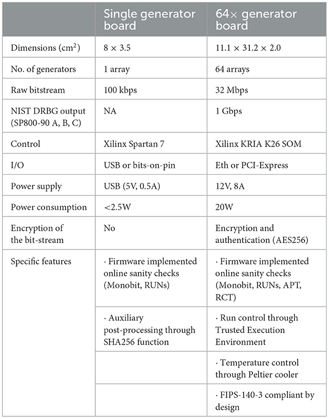
Table 1. Table of specifications for the two embodiments of the silicon-based QTRNG under consideration on which the online health tests were firmware implemented: the single generator board and the 64 × x generator board.

Bit streams are generated by analyzing the time series of self-amplified endogenous pulses in Silicon PhotoMultipliers (SiPMs). These pulses originate from stochastically generated charge carriers in an array of p-n junctions operated beyond their breakdown voltage, mimicking the statistics of radioactive decay events. The physical mechanism is well modeled in semiconductor theory: charge carriers randomly crossing potential barriers enter a high electric field region and trigger an avalanche multiplication by impact ionization in the Geiger-Müller regime. A full description of the underlying processes can be found in reviews of SiPM physics (McKay, 1954; Senitzki B., 1958; Haitz, 1965). Using SiPMs as entropy sources ensures compactness and robustness: pulses are large (millions of electrons) and short (tens of nanoseconds), which enables precise time-tagging and efficient bit extraction without the need for additional post-processing.

The hardware implementation of these principles is shown in Figure 1. Each board integrates the SiPM detector array, biasing, temperature control and/or compensation features, a proprietary time-to-digital converter (TDC), and a field-programmable gate array (FPGA) responsible for bit extraction and health monitoring.

Figure 1

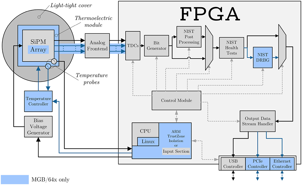
Figure 1. General overview of FPGA-based QTRNGs developed by RandomPower (Caccia et al., 2020). The stochastic impulses are generated by the SiPM. A dedicated analog circuitry (substituted by a dedicated chip in the 64×) implements the triggering logic, generating a digital signal that is fed directly into the FPGA. Inside the FPGA, it is timestamped by a dedicated TDC, and the timestamps are then analyzed by the bit generator to produce four-bit symbols. Optional post-processing, in the form of a SHA-256 whitening accelerator, can be applied to remove any residual bias if needed. After passing through the Health Test accelerator (implementing Monobit, RUNS, APT, and RCT), the bit-stream can be routed through a NIST-compliant DRBG. The resulting output may then be directed to the USB interface (in the case of the SGB) or to the Ethernet/PCIe interface (in the case of the 64 × ). ARM TrustZone ensures isolation of the control logic and allows only approved applications to manage the process. The main difference between the 64× and the SGB is highlighted in light blue: the 64× integrates a temperature controller and thermoelectric module to stabilize the array at a specified temperature.

The prototype implementation replaces discrete commercial TDCs with an embedded FPGA TDC IP Core. The inclusion of the TDC within the FPGA fabric, as shown in Figure 1, allows for on-the-fly updates and tweaks as the device development improves. This design was chosen to increase throughput and upgradability and to reduce costs and possible attack surfaces (Fagan et al., 2025). Generally, the process of time stamping is performed with external TDCs; however, this increases complexity and decreases flexibility. Additionally, the temperature-dependent calibration logic allows for removing the non-linearities generated by temperature shifts.

The FPGA TDC converts electrical impulses to random bit streams by analyzing inter-arrival times of nine-pulse series to generate four-bit sequences, resulting in an alphabet of 2⁴ = 16 possible symbols for each cycle.

It is worth noting that correlations during the generation process, dead times of the QRNG during time stamping of the pulses, and external factors, such as thermal runaways, may introduce time-dependent anomalies in the generation of bits or symbols, making the implementation of efficient, near real-time health tests a very relevant tool for assessing the quality of the generated sequences.

4 The IID procedure

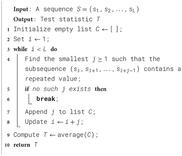
The main metric for the evaluation of the randomness of a bit-stream is given by the measure of the minimum entropy, which is described in document (Turan et al., 2018) and is subject to the assumption that the symbols that make up the stream are independently and identically distributed (the IID hypothesis in the following). The NIST procedure to assess the latter, detailed in Chapter 5 of the same document, is based on a bootstrapping method performed on eleven statistical tests that can be grouped into the excursion test statistic, statistics on runs, statistics on collisions, periodicity and covariance tests, and the compression test. The pseudo-codes as described in NIST documentation for a representative from each category are outlined below in Algorithms 1–5, respectively.

Algorithm 1

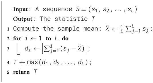
Algorithm 1. Excursion test statistic.

Algorithm 2

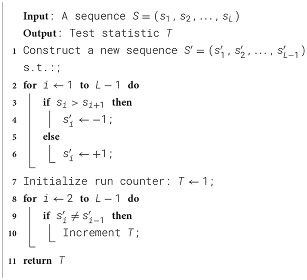
Algorithm 2. Number of directional runs.

Algorithm 3

Algorithm 3. Average collision test.

Algorithm 4

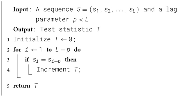
Algorithm 4. Periodicity test.

Algorithm 5

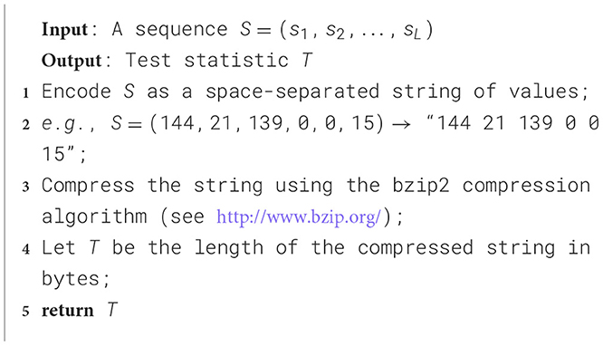
Algorithm 5. Compression test statistic.

A sequence of length n_symbols is taken as input for the above statistical tests. The outcomes (hereinafter referred to as Tx) are taken as reference and used to compare the results of the aforementioned tests on a shuffled set of the input sequence obtained via Fisher-Yates shuffle algorithm: whenever the latter (here called Ti) are greater than Tx, a counter C0 is updated; if they are equal to Tx, a second counter C1 is updated. Such counters are evaluated independently for each test, and a number n_sequences of shuffled sequences is tested. The symbols are validated as IID if, for every test, both C0≥0.0005*n_sequences and C1+C0 ≤ 0.9995*n_sequences (i.e., if the reference value Tx does not lie in the upper or lower 0.05% of the total population of Ti.). This is actually a generalization inferred from the parameters provided in the NIST documentation, as the standard procedure considers only the fixed values n_symbols= 10⁶ and n_sequences= 10⁴, with thresholds for IID validation of C0≥5 and C1+C0 ≤ 9995. The procedure is outlined in Algorithm 6.

Algorithm 6

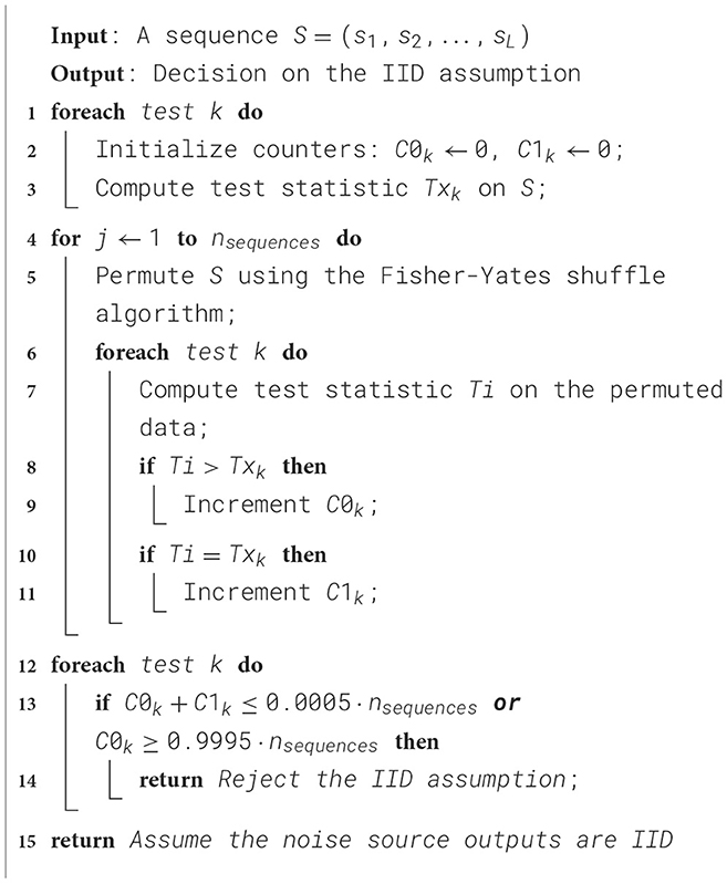
Algorithm 6. Permutation based procedure to test the IID Assumption.

For a fixed test, the population of the Ti considering n_symbols= 10³ and n_sequences= 10⁵ is shown as a histogram in Figure 2. The reference value Tx is marked by a red line.

Figure 2

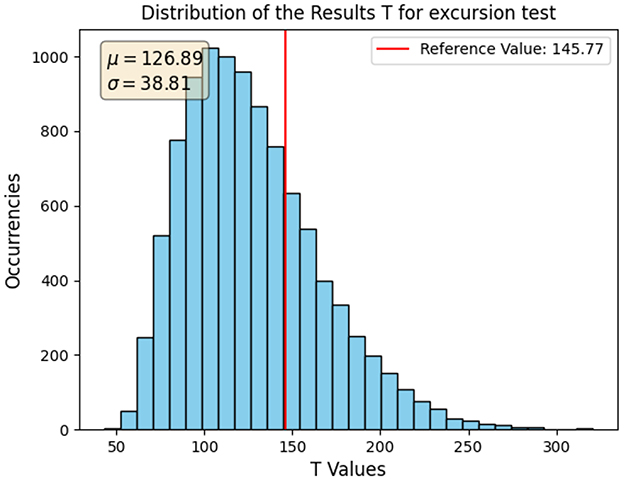
Figure 2. Histogram of the Ti population for the excursion test on 10⁵ sequences of 10³ symbols each. The reference value Tx associated with the input sequence is marked by a vertical red line, and the mean and standard deviation of the population are reported on the graph.

One can already get a qualitative assessment by observing that the reference value Tx is not as far toward an edge of the axes to disprove the IID assumption. As far as that is concerned, however, Tx could just as well fall within the greater 10% of the Ti population: the outcome of the Boolean conclusion on IID behavior would be the same, but the probability for the counter C0 to increase at each iteration would be greatly affected. This aspect was taken into consideration in the statistical analysis developed in the following, which is not a part of any NIST documentation.

The IID tests described by NIST, albeit concise and simple, cannot be easily evaluated in terms of a theoretical distribution of their outcomes. To perform a critical statistical study of the results, understand the NIST procedure, and test the implementation done, an approach similar in spirit to what is done by NITS in the IID evaluation itself is developed. Instead of comparing the distribution of the values Ti obtained in a single run, the distribution of the counter C0 across multiple runs is considered. The latter is assumed to be binomial, with a probability of success p (i.e., the increase of C0) given by the relative value of the reference result Tx.

In this section, the parameters for a single run (i.e., a single value of C0) are n_symbols = 10³ and n_sequences = 200, repeated a number n_iterations = 500 of times. These values are chosen to fully use one of the 250MB files generated by our QRNG in the following steps while leaving some buffer, keeping both the population of the histogram and the space of the results Ti, respectively, high and wide enough for the results to be meaningful. The reason for including this buffer will become clear shortly, as an additional test introduced later requires it. The same parameters were maintained for consistency in the analysis.

Figure 3A displays the results for the excursion test: the blue dots outline the distribution of the measured C0 (each is accompanied by its binomial error), while the red line represents the theoretical binomial distribution they are supposed to follow. The box on the graph reports the mean and standard deviation of the dataset, the probability of success p for the increase of the counter C0 (computed as the relative position of the reference value Tx with respect to the population Ti, i.e., in which percentile of the population stands the red line in Figure 2, and used to compute the theoretical binomial distribution), and the value of the reduced χ² for the dataset under the null hypothesis of them following the red binomial distribution.

Figure 3

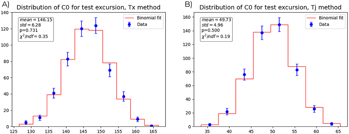
Figure 3. (A) Distribution of 500 counters C0 for the excursion test, each computed over 200 sequences of 10³ symbols and evaluated with respect to the value of the input sequence. The observed distribution is shown by blue dots with binomial error bars, and its mean and standard deviation are reported in the box. The probability of increase of the counter C0 p, computed a priori, is used to plot the theoretical expected binomial distribution in red. The reduced chi-square of the data with respect to this binomial is reported in the box. (B) Distribution of 500 counters C0 for the excursion test, each computed over 200 sequences of 10³ symbols and evaluated with respect to the value of the previous sequence considering disjointed pairs. The observed distribution is shown by blue dots with binomial error bars, and its mean and standard deviation are reported in the box. The probability of increase of the counter C0 p, equal to 0.5 by construction, is used to plot the theoretical expected binomial distribution in red. The reduced chi-square of the data with respect to this binomial is reported in the box.

Throughout the previous analysis, the fact that the value Tx was taken as reference for all the following ones put the input sequence in a very special position. As it was briefly mentioned, such value is effectively picked at random, thus having the potential of skewing significantly the binomial distribution of the counter C0, whose probability of success parameter p can vary significantly with the sole requirement of being 0.0005 ≤ p ≤ 0.9995. To bypass the special role given to the first sequence and have a predictable and uniform value for p throughout the tests and the tested files, a second ratio for the increase of C0 is developed, to which we refer as TjNorm. Instead of having a fixed reference, the sequences are evaluated in pairs: given a statistical test, the counter C0 is increased whenever the result on the jth sequence is greater than the one on the jth+1 sequence. If such results turn out to be equal, the pair is discarded, so that the results are normalized and the probability of increase of the counter C0 is p = 0.5 in each iteration. The need to provide some buffer to account for the fact that some sequences will probably be ignored forces us to lower either the values of n_symbols, n_sequences, or n_iterations from those that would fit in the 250 MB file analyzed.

With this new method, Figure 3B was plotted, with parameters n_symbols = 10³, n_sequences = 200 and n_iterations = 500. These values were chosen giving priority to n_iterations being high enough for the statistical interpretation to be relevant and to n_symbols = 10³ being high enough so that the space of the results of the tests (i.e., what was previously called the Ti) would be wide enough. This is the equivalent of Figure 3A and it is to be interpreted in the same way. Just a caveat: the mean value of the distribution is correctly 50, with n_sequences = 200 and p = 0.5, because, as the sequences are evaluated in pairs, they give an effective halved number of values of C0 compared to their previous “Tx method” counterpart.

After a bitstream has been validated as IID, its minimum entropy can be easily calculated as H_min = −log(p_max), where p_max is the frequency of the symbol that is the most likely to occur. The NIST prescription described in (Turan et al. 2018), chapter 6, actually considers a lower bound on this quantity by taking the highest bound on p_max at 2.576 sigma CL (corresponding to a z value at 0.995). Figure 4 shows the frequencies of the symbols compared to the uniform distribution (red dashed line) for a 250MB file generated by our QRNG; each is accompanied by its binomial error. The resulting minimum entropy is 3.9997 ± 0.0002, where the uncertainty was obtained by propagating the binomial uncertainty of p_max, and the lower bound on it, as computed following NIST standards, is 3.9991. Both are displayed on the graph.

Figure 4

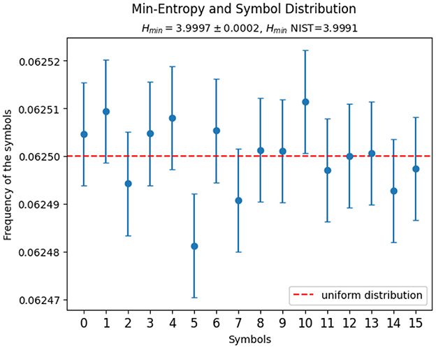
Figure 4. Scatterplot of the frequencies of the four-bit symbols in a 250MB file generated by the QRNG under consideration and consequent evaluation of the minimum entropy. Each frequency is accompanied by a binomial error bar and the expected uniform distribution is plotted as a red dashed line. The minimum entropy H_min and the estimation for minimum entropy according to NIST guidelines H_minNIST are reported. The first is accompanied by an uncertainty obtained by propagating the binomial uncertainty on p_max, while the second is a lower bound estimate that considers an upper bound on p_max at 99.5% CL.

The Python implementation of the procedure for evaluating the IID assumption, the statistical analysis performed to assess it (which can also serve value as validation of the implementation) and the computation of the minimum entropy is made available in a public GitHub repository.¹

5 Standard online statistical tests

The anomaly detection procedure, presented in Section 6, is based on a set of four wellknown and recognized tests, operating on single sets of bits or symbols. The Monobit and RUNS tests were selected from the numerous tests within the NIST test suite based on their simplicity, which is essential for a firmware implementation, and the complementary information they offer. Specifically, the Monobit test assesses the asymmetry of bit distribution within a bit-string, whereas the RUNS test quantifies the occurrence of bit-flips. Due to their minimal correlation, these tests maximize the information inferred from the data. These two tests find their natural generalization to symbols of multiple bits, respectively, in the adaptive proportion and the repetition count tests, which are defined by NIST in (Turan et al. 2018) and used to assess the eligibility of a sequence to seed a DRBG.

5.1 Symmetry tests

5.1.1 Monobit

The Monobit test (Rukhin et al., 2001) asserts the asymmetry between zeros and ones in a bit sequence. Given a set of n bits, the stochastic variable is defined as

$\begin{array}{ll}{S}_n={\displaystyle \sum _{i=1}^n}{x}_i=2n_1-n& (1)\end{array}$

where x_i = 2ϵ_i−1, ϵ_i is the bit state and n₁ is the number of 1s in the bit sequence. Provided that the bit values are independent and identically distributed, the number of bits set to 1 follows the binomial probability density function:

$\begin{array}{ll}B(n_1,n,p)=\frac{n!}{n_1!(n-n_1)!}{p}^{n_1}{(1-p)}^{n-n_1},& (2)\end{array}$

with p being the probability of generating 1. If both values are equally probable, then $\overline{S_n}=0$, with standard deviation ${\sigma }_{S_n}=\sqrt{n}$. The Monobit test fails whenever a sequence has a value S_n that exceeds an alarm level $k\sqrt{n}$, where k is defined according to the sensitivity and false alarm rate set by the user.

5.1.2 Adaptive proportion test

The APT expands upon the binary checks performed by the Monobit test to include an alphabet of m symbols. As defined in the NIST documentation (Turan et al., 2018), the stream is divided into sequences of length n. The frequency of the occurrence of the first symbol is checked against the hypothesis of a binomial distribution with p = 1/m.

Specifications for the sequence length to be considered are specific to the alphabet used and are provided by NIST. For binary sequences, the recommended length is n = 1, 024, while for non-binary sequences, it is suggested to use n = 512. Within each sequence, the occurrences of the first symbol are counted and compared to a cut-off threshold corresponding to a defined failure probability. The cut-off threshold can be calculated relying on the binomial cumulative distribution function, assuming an equal probability for each of the m symbols to be generated.

5.2 RUNS tests

5.2.1 RUNS

This test counts the number of series of consecutive identical bits in a sequence of specified length, as shown in Figure 5. It is worth noting that this quantity can be measured by the number of bit flips plus one.

Figure 5

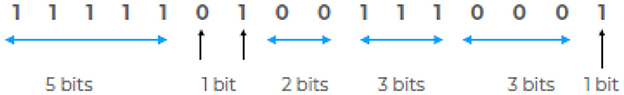
Figure 5. The RUNS test counts the number of sequences of consecutive identical bits in a bit-stream. In this figure, a sequence of n = 16 bits containing a total of seven runs is shown.

This test complements the Monobit: for a given value of n₁, it measures the expected number of bit flips in the sequence under the hypothesis of a “fair coin.” The underlying probability distribution is the probability of having runs of a specific length conditioned on the number of ones in the sequence with p = 1/2. By defining

$\pi =\frac{n_1}{n}$

as the fraction of bits set to 1, the average number of runs and the variance are given by (Bradley 1968)

$\begin{array}{l}\overline{R}=2n\pi (1-\pi )+1,\\ {\sigma }_R^2=\frac{n}{n-1}\times [2\pi (1-\pi )(2n\pi (1-\pi )-1],& (3)\end{array}$

corresponding to the first and second moments of the underlying probability distribution function. Ultimately, the purpose of this test is to determine whether the oscillation between sub-sequences of identical bits is too fast or too slow compared to the expectations (Soto and Bassham, 2000). As for the Monobit, whenever a sequence exceeds a threshold value $\overline{R}\pm k{\sigma }_R$, the test is considered failed.

5.2.2 Repetition count test

The RCT also relies on the concept of runs, generalizing the test to sequences of symbols. However, instead of counting the number of symbol changes, it focuses on the length of consecutive identical instances.

The probability α of having at least C consecutive equal symbols can be written as:

$\begin{array}{ll}\begin{array}{c}\alpha =P(k\ge C)={\displaystyle \sum _{i=1}^m}(1-p_i)p_i{p}_i^{C-1}={\displaystyle \sum _{i=1}^m}(1-p_i)p_i^C\end{array}& (4)\end{array}$

where k is the length of the runs, p_i stands for the probability associated with the i-th symbol of the alphabet, and (1−p_i) represents the probability of the symbol generated before the current one being different, resetting the counter of the length of the run. Assuming p₁ ≥ p₂ ≥....≥ p_m, Equation 4 can be given an upper bound by:

$\begin{array}{ll}\alpha =P(k\ge C)\le (m-1)·p_1^C=(m-1){(2^{-H})}^C,& (5)\end{array}$

where H is the min-entropy defined as H = −log₂(max{p_i}) (Turan et al., 2018). Once the value of α is defined, the cut-off threshold C can then be computed as:

$\begin{array}{ll}C=\lceil \frac{1}{H}\left[lo{g}_2(m-1)-lo{g}_2(\alpha )\right]\rceil & (6)\end{array}$

It should be noted that Equation 6 differs from the original NIST prescription as a consequence of the implementation, which is based on the assumption that the symbols are being analyzed sequentially. Consequently, it embodies the viewpoint of the “observer symbol,” which must differ from the preceding one and match the subsequent C−1 symbols.

NIST recommends choosing the α parameter between 2⁻²⁰ and 2⁻⁴⁰, equivalent to, respectively, a 5σ and a 7σ confidence level, presuming a Gaussian distribution of the measured quantities. In this work, a value of α = 2⁻²⁰ is chosen.

6 Anomaly detection procedure and experimental results

The anomaly detection framework proposed in this work departs in scope and intent from the health tests described in the previous section. NIST defines the repetition count and adaptive proportion tests as lightweight monitors intended solely to detect catastrophic failures of the entropy source, with each failure leading to the rejection of the sequence under test. In contrast, our procedure extends these tests, together with the Monobit and RUNS statistics, into a statistical framework that evaluates series of test outcomes. Rather than discarding each failing sequence, we accumulate results to distinguish between sporadic fluctuations, statistically expected in any random source, and persistent deviations that indicate a systematic bias. This shift from single-sequence rejection to distribution-based monitoring enables online detection of long-term drifts in source quality while simultaneously supporting an estimation of entropy that can be cross-checked against NIST's min-entropy bounds.

Once a sample of results from the health tests on N series of n bits (or symbols) is collected, procedures are developed and commissioned with the aim of identifying long-term drift or otherwise assessing the randomness quality.

The inter-failure sequence number ($\overline{ISN}$) is introduced, which represents the average measured number of sequences between two failures. This measure is employed as a qualifier for the tests.

6.1 Monobit

The diagnostic power of the Monobit on single bit-strings can be assessed as the capability to detect anomalies in the number of ones n₁ in a sequence of n random bits, as those result in an absolute value of S_n in excess of kσ_Sn, where k determines the confidence level. This condition can be written as:

$\begin{array}{l}{S}_n\ge k\sigma \Rightarrow (2n_1-n)\ge k\sigma \\ \Rightarrow n_1\ge \frac{1}{2}(k\sqrt{n}+n).& (7)\end{array}$

If j bits are forced to one, the alarm is triggered whenever the number of ones in the remaining n−j random bit string $n_1^{n-j}$ is

$\begin{array}{ll}{n}_1^{n-j}\ge \frac{1}{2}(k\sqrt{n}+n)-j.& (8)\end{array}$

The rate at which this happens can be computed as the tail of the distribution of $n_1^{n-j}$ and represents the true positive probability (TPP) for Monobit fails; on the other hand, the false positive probability (FPP) is associated with the statistical distribution of n₁ for an unbiased string. The comparison between these two quantities over a sequence of n = 32 bits at varying confidence levels (ranging from 0 to 4σ) is illustrated in Figure 6. Notably, the sensitivity is close to 50% unless the number of biased bits grows to a significant fraction. On the other hand, the analysis of a series of S_n values can lead to a procedure enhancing the TPP, thus providing a basis for anomaly detection with single-bit precision.

Figure 6

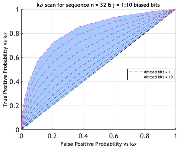
Figure 6. Sensitivity scan of the Monobit test across different confidence levels for a sequence of length n = 32 bits with a number j of biased bits ranging from 1 to 10. For a fixed number of biased bits, the corresponding curve is obtained by plotting the false positive probability vs true positive probability for a kσ threshold, with k varying from 0 to 4. To meaningfully distinguish between a true positive and a false positive warning for bias on a single sequence, the number of corrupted bits must be a significant fraction of the total. This brings us to consider the mean of the Monobit results over a series of sequences as the relevant statistics.

This consideration can be extended to all the tests described in the previous section, driving the shift in focus from the assessment of a single string to the statistical analysis of a series of N sequences of n random bits. This approach is aimed at an online differentiation between systemic failures, which indicate a bias in the source of bits, and occasional failures caused by statistical fluctuations.

The observable considered is $\overline{S_n}$, the average value of S_n over N sequences, which is expected to be Gaussian distributed because of the central limit theorem. A bias model is introduced by setting j bits to 1 and, as outlined in Figure 7, two potential bias indicators can be considered: a normalized shift of the average value and a variation in the fraction of events in the distribution's tails. Presuming every sequence to be biased, the dependence of the shift on the number j of biased bits is linearly dependent on j, in fact

$\begin{array}{l}{S}_n=2n_1-n=2(n_1^{n-j}+j)-(n^{n-j}+j)=\\ =(2n_1^{n-j}-n^{n-j})+j& (9)\end{array}$

and $E\left[\overline{S_n}\right]=j$, eventually scaled by the fraction of biased sequences in the series. On the other hand, the fraction of events in the tail is expected to be non-linearly dependent on j, since it is the integral of the normalized $\overline{S_n}$ distribution above the threshold value k. The sensitivity of the two measures is presented in Figure 8 for an exemplary sequence length n = 32 as the number of biased bits changes. The biasing frequency ranges from every sequence to one in every thousand, across series of N = 2⁵ sequences. Results prove that the $\overline{S_n}$ shift estimator outperforms the method of counting events in the tails. Setting a k = 3 confidence level, the effect of a single biased bit can be detected for tampering frequencies higher than one in 10 sequences, while at least five biased bits are required when one in 100 sequences is biased, and sensitivity is limited for lower frequencies unless a higher statistic is considered.

Figure 7

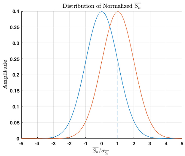
Figure 7. Exemplary distributions of the normalized mean outcomes $\overline{S_n}$ of the Monobit test for an unbiased (in blue) and biased (in red) bit stream. The bias introduces an asymmetry between the 0s and the 1s that results in a shift of the distribution from the expected. Two metrics can be considered to distinguish the two: the shift in the mean value of the distribution and the number of events in the tails over a fixed threshold, here illustrated by the dashed line.

Figure 8

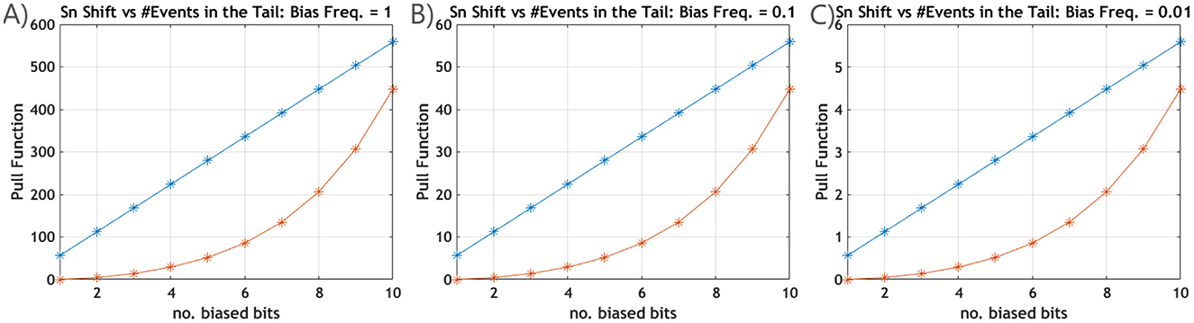
Figure 8. Comparison between the sensitivity of the estimators in the detection of a bias for the Monobit test: the shift of the mean value of $\overline{S_n}$ (in blue) is evaluated against the variation in the number of anomalies expected (in orange), calculated as the integral of the distribution of events in the tails over the 3σ limit, when a number of bits is forced to 1. The comparison is performed with the bias being introduced in every sequence (A), once every 10 sequences (B), and once every 100 sequences (C). The value of the pull function with respect to the unbiased sequence for the two estimators consistently identifies the shift on the mean value of S_n as the most sensitive.

The features of the $\overline{S_n}$ distribution are the basis of the online assessment of the quality of the bit-stream produced by the generator. If the $\overline{S_n}$ of the current series exceeds the 3σ threshold, a false positive warning is raised. The threshold was chosen as a trade-off with the sensitivity to the errors detected. If it is set too low, too many False Flags will be detected, while too high a threshold might not detect actual malfunctions. Therefore, the trade-off was set to a threshold of 3σ, corresponding to a 99.9% confidence level or false flag probability of 10⁻³. The joint probability of having two consecutive uncorrelated warnings is approximately 10⁻⁶, while the probability of three is 10⁻⁹. Therefore, the likelihood of such occurrences is negligible unless a bias in the generation process is present.

A 1 Gb sample is partitioned into series, each with N = 2¹⁷ sequences of n = 32 bits. As shown in Figure 9, the $\overline{S_n}$ trace plot during online production indicates no catastrophic failures of the entropy source, despite a single warning being triggered by statistical fluctuations. The strength of this method lies in its ability to detect systematic failures of the entropy source during online generation and to promptly alert the user of the malfunctions.

Figure 9

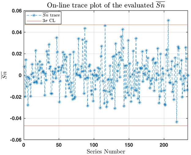
Figure 9. Trace plot of the computed mean of the Monobit statistics $\overline{S_n}$ during online production over a number of series of N = 2¹⁷ sequences of n = 32 unbiased bits each for a total of 1 Gb. The orange horizontal lines represent the 3σ confidence level of deviation from the expected value that act as thresholds: a value of $\overline{S_n}$ outside the range raises a warning; three consecutive warnings signal a catastrophic failure in the bit generation.

Moreover, a retrospective analysis is performed on the properties of the distribution of the number of sequences in between two failures (inter-failure sequence number, ISN). The average value of ISN clearly depends on the threshold value over which a failure is declared, as reported in Table 2, so to have a large statistic of failures, the analysis is performed by setting k = 1. Results are shown in Figure 10, where the trend is fitted with the model

$\begin{array}{ll}P(X=x)=p{(1-p)}^{x-1},& (10)\end{array}$

which describes the probability P of having the next failure after x sequences, with p being the failure probability. Results are statistically compliant with the hypothesis of an unbiased distribution, as confirmed by the total number of failing sequences in 1 Gb of data (measured to be 74.6 ± 2.6 against an expected value of 77).

Table 2

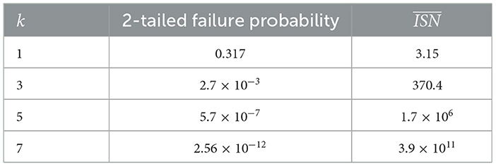
Table 2. Expected ISN (i.e., $\overline{ISN}$) given kσ CL in a normal distribution.

Figure 10

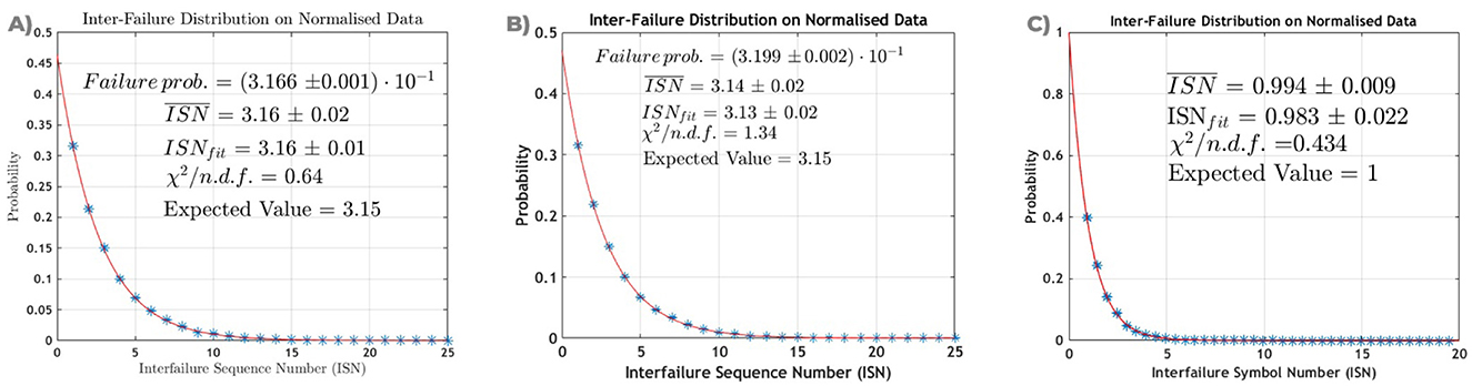
Figure 10. Normalized occurrences of the ISN, i.e., the number of sequences between two consecutive failures, with the threshold set at 1σ for (A) the Monobit test, (B) the RUNS test, and (C) the RCT test. The blue datapoints are fitted with the orange line, and the goodness of fit is evaluated via the reduced chi-square. The mean value of the dataset $\overline{ISN}$ is then compared with the value computed from the fit ISN_fit. The ISN for the Monobit test (A) and for the RUNS test (B) are evaluated over 1 Gb of random bits generated with the QRNG under consideration and fitted assuming that the probability for it to be equal to x is P(ISN = x) = p(1−p)^x−1, with p being the failure probability reported on the graph. Both ISN_fit and $\overline{ISN}$ are compatible with the expected value for an unbiased bitstream. The ISN for the RCT test (C) is evaluated over a sample of 100 Gb of random bits and fitted assuming an exponential trend. Both ISN_fit and $\overline{ISN}$ are compatible with the expected value for an unbiased bitstream.

6.2 RUNS

As for the Monobit, a collection of RUNS values was used to define a diagnostic tool for biases and systematic failures by analyzing samples of N sequences of n bits. It is reasonable to assume that the considerations previously outlined for the Monobit persist, so the analysis is focused on the shift of the average of the measured number of runs from the expected mean. As the latter depends on the actual number of ones n₁ present in the sequence, a normalized shift is considered instead: For each sequence, the measured number of runs R_m is replaced by the z-score

$\begin{array}{ll}z=\frac{R_m-\overline{R}}{\sigma },& (11)\end{array}$

which is expected to exhibit a Gaussian behavior by the central limit theorem. Unbiased series of N sequences are expected to be centered around $\overline{z}=0$.

Following the same approach as the Monobit test, the investigation of the sensitivity of the RUNS test is performed by introducing a bias in the number of runs in the sequences. By defining

$\begin{array}{l}\overline{z}=\frac{1}{N}{\displaystyle \sum _{i=1}^N}{z}_i,\\ {\sigma }_{\overline{z}}=\frac{1}{\sqrt{N}},& (12)\end{array}$

presuming the sequence to be biased, an average change by ΔR in the number of runs will induce a variation

$\begin{array}{ll}\text{Δ}\overline{z}=\frac{\text{Δ}R}{{\sigma }_{\overline{z}}},& (13)\end{array}$

which can be identified as long as $\left|\text{Δ}\overline{z}\right|\ge k·{\sigma }_{\overline{z}}$ where k is set according to the required confidence level. The threshold at k standard deviations from the expected value of number of runs in a series is, therefore,

$\begin{array}{ll}\left|\text{Δ}R\right|\ge k·\frac{1}{\sqrt{N}}.& (14)\end{array}$

The shift of the z-score due to the bias, with a frequency of once every 10 sequences, could be detected with single-bit precision at a confidence level of up to 5σ. As reported in Table 3, this level of accuracy in sensitivity is maintained for sequences up to 128 bits long, while for longer sequences—or equivalently for a lower frequency of the bias—the sensitivity is limited and the test requires a larger deviation ΔR from the expected average to spot the bias.

Table 3

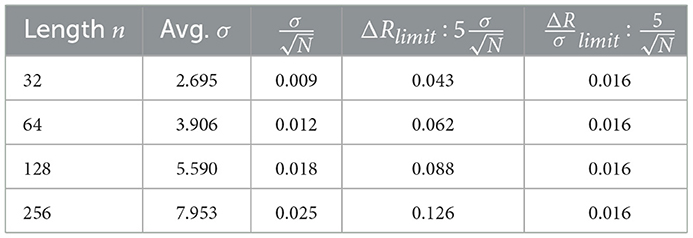
Table 3. Sensitivity of the RUNS test at 5σ CL for ΔR variations of the number of runs, by analyzing 10⁵ unbiased sequences and computing the average σ.

Experimental results from the online evaluation of the z-score are displayed on the trace plot of Figure 11. In the absence of catastrophic failures, the computed z-scores remain within the expected confidence level, except for the expected statistical fluctuations.

Figure 11

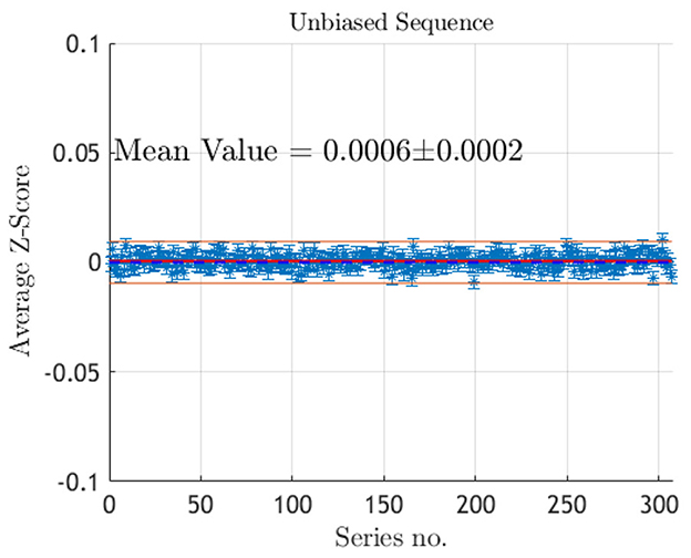
Figure 11. Trace plot of the z-scores with associated error bars for the RUNS test computed online during production over 307 series of N = 2¹⁷ sequences of n = 32 unbiased bits. The red dashed line indicates the expected value for a random bitstream and the orange lines mark the warning thresholds at 3σ. With this choice, 0.3% of the population is expected to generate warnings: the observed count of 1 warning over 307 series aligns with this expectation.

Further analysis is conducted by measuring the ISN, employing the same dataset and setup parameters as the Monobit test. The results of the dataset provided by the considered architecture are statistically compliant with the hypothesis of an unbiased distribution, and are reported in Figure 10.

These findings indicate that, similarly to the Monobit test, the RUNS test is reliable for the online identification of systematic failures of the system during production. These failures cause the distribution to shift significantly from the expected value and can be detected with a relatively small sample size.

6.3 Repetition count test

The repetition count test is approached in a statistical framework by examining the properties of the distribution of the ISN, with the aim of assessing the quality of the bit-stream in terms of the min-entropy H. Due to the large amount of data necessary, this analysis is conducted retrospectively, rather than being performed online. However, it implies no extra computational costs since it uses data already collected from tests required by NIST specifications for the DRBG procedure.

As per NIST recommendations, the failure probability α is set to 2⁻²⁰; this, together with the previously mentioned fact that the architecture under scrutiny provides four-bit symbols, sets the threshold for the number of consecutive identical symbols to C = 6, as reported in Table 4. Failures within a defined window are, therefore, expected to be driven by the Poisson distribution, with the number of sequences between two occurrences being exponentially distributed.

Table 4

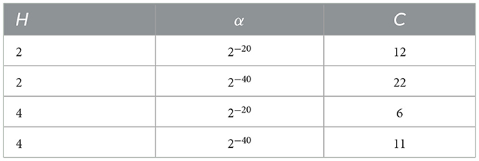
Table 4. Exemplary cut-off thresholds for multiple H and α values, given m = 16.

Over 100 Gb of random bits generated by each of four silicon-based QRNG boards are considered, divided into three sets for each board. To avoid floating-point approximation problems associated with exponentials with extremely low numbers, the measures were scaled with respect to the expected $ISN=1/\alpha =2^{6·4-lo{g}_2(15)}$ obtained by applying Equation 6 with C = 6 and H = 4. As a matter of fact, the observed ISNs, normalized over the number of failures, conform with the exponential hypothesis, as shown by the fit in Figure 10, with the computed parameter for the exponential distribution consistently falling within the 99.7% confidence interval of the expected value for an unbiased source.

The measured entropy H and an estimation of the min-entropy are evaluated starting from $\overline{ISN}$. The measured entropy is obtained by substituting in Equation 6 the measured average failure rate $\overline{\alpha }=1/\overline{ISN}$, as C is fixed, and the uncertainty is computed by propagating the error:

$\begin{array}{ll}{\sigma }_H=\frac{1}{Cln2}\frac{1}{{\sigma }_{\alpha }}.& (15)\end{array}$

As the statistic on the number of failures is sufficiently large, the $\overline{ISN}$ is assumed to approximately follow a Gaussian distribution with standard deviation equal to ${\sigma }_{\overline{ISN}}=\sqrt{n_{fails}}$, where n_fails denotes the total number of failures in the sample. To determine a lower bound on the min-entropy, a shift of $3{\sigma }_{\overline{ISN}}$ to the right of the average is considered to recover the largest possible true value of α (hereby denoted as $\tilde{\alpha }$) compatible with a 99.7% confidence to the observed one:

$\begin{array}{ll}\frac{1}{\tilde{\alpha }}=\widetilde{ISN}=\overline{ISN}-3{\sigma }_{ISN}.& (16)\end{array}$

This value is then substituted in Equation 6 to get the corresponding limit on the entropy. The results are reported in Figure 12, where different cut-off thresholds C = 6, 7, 8 are considered. Notably, the measured entropy does not consistently adhere to its physical constraints, reflecting the heuristic nature of the collected data, where the number of failures fluctuates. The reported min-entropy estimation represents the minimum entropy value that aligns with the measured outcome, computed by applying the aforementioned 3σ shift of the measured value. Taking C = 6, this lower bound consistently falls between 3.989 and 3.998 for each of the subsets of samples considered for all the boards. With an increase in the cut-off threshold, the probability of encountering a failing run diminishes, thus resulting in a larger uncertainty.

Figure 12

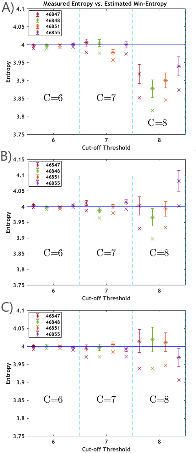
Figure 12. The plots exhibit the measured entropy, labeled as *, with the related uncertainty, and the min-entropy estimation, labeled as ×, which corresponds to the lower bound on the measured entropy given a 99.7% confidence. The theoretical limit H = 4 for a perfectly entropic stream of four-bit symbols is marked by the blue continuous line. The values were computed on 100 Gb of data produced with generators #46847 (red), #46848 (green), #46851 (orange), and #46855 (purple), divided into three sets [reported in (A–C), respectively], by running the RCT test with three values of the cut-off threshold C. For C = 6, the min entropy estimations consistently fall between 3.989 and 3.998. Increasing the cut-off threshold diminishes the number of failures, thus increasing the error.

6.4 Adaptive proportion test

The analysis of the APT follows the same statistical approach as the RCT to estimate the min-entropy. As defined by NIST guidelines, the data are partitioned into sequences of n = 512 symbols. The number of occurrences of the first symbol within each sequence is counted, and the test is failed if the count exceeds a set threshold C. The failure probability, therefore, follows a binomial cumulative distribution function (B_cdf):

$\begin{array}{ll}P(k\ge C)=B\text{\_}cdf(C-1,N-1,p),& (17)\end{array}$

where p is the probability of occurrence of the selected symbol, and the −1 in the first and second arguments is due to the first symbol being fixed and already accounted for. Assuming an unbiased bit-stream, $p=\frac{1}{16}$. Instances where the frequency of occurrences for the first symbol falls below a lower threshold are also considered. In such cases, the corresponding binomial cdf is included in Equation 17 to compute the overall failure probability. In this setting, given the failure probability α = 2⁻²⁰ and m = 16, the test is deemed unsuccessful if the count of a symbol exceeds C≥62 or is smaller than C ≤ 8. The observed results, obtained by varying the cut-off threshold, are plotted in Figure 13 and compared with the theoretical binomial cumulative distribution, to which they comply.

Figure 13

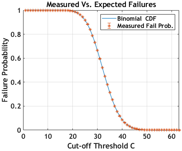
Figure 13. The performance of the APT for different values of the cut-off threshold over the unbiased bit-stream generated with our QRNG is reported in orange. The datapoints consistently lie within 3σ from the expected value given by the binomial cumulative distribution function, which is plotted in blue.

The failure probability is linked to the probability of occurrence of a symbol p, which yields the bit-stream entropy as H = −log₂(p). Figure 14 displays an estimated p = 0.0627 ± 0.0002 based on measured failures and binomial error. Table 5 provides a summary of the measured entropy values and their uncertainties. By taking the weighted average for each set from each board, the lower bound on the entropy within a 99.7% confidence level is H(#46847) = 3.9917, H(#46848) = 3.9724, H(#46851) = 3.9842, and H(#46855) = 3.9824.

Figure 14

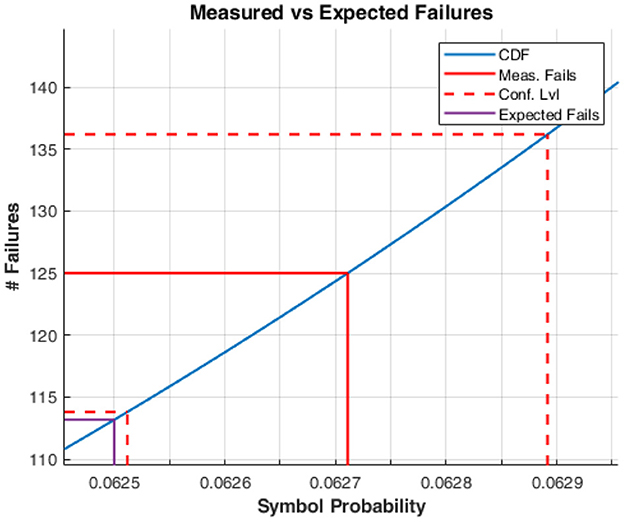
Figure 14. The estimation of the entropy H of the bit-stream as a sequence of four-bit symbols is computed by evaluating the probability p of occurrence of the most frequent symbol as the measured number of failures of the RCT on the bit-stream. The observed number of failures is traced back by the red continuous line to the corresponding p on the cumulative distribution function that governs the RCT (in blue). The result is accompanied by an uncertainty obtained by tracing back a one sigma binomial error on the observed number of failures (red dashed lines). The computed p is p = 0.0627 ± 0.0002. The purple line marks the expected fails for the theoretical limit H = 4. Taking the +3 sigma value for the number of failures gives a lower bound for the entropy of the bit-stream of 3.983 at a 99.7% confidence level.

Table 5

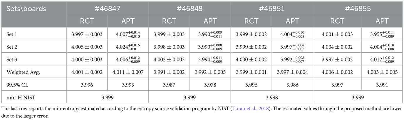
Table 5. A comprehensive report on the measured entropy for the RCT and APT for α = 2⁻²⁰, showing that all values fall within the theoretical entropy limit, considering statistical fluctuations during the generation process, and assuming an unbiased bit-stream.

The investigation on the APT could be extended by evaluating the occurrences of every symbol in the alphabet under consideration. In fact, such an integration is further validated by the fact that the minimum entropy is linked to the occurrence rate of the most probable symbol. Likewise, the failure probability for each symbol is assumed to be binomial. However, potential correlations between the symbols could significantly affect the number of failures recorded. Assessing these correlations and defining precise thresholds is necessary and will be addressed in future work.

7 FPGA implementation of the anomaly detection procedure

The anomaly detection procedure outlined in Sections 5 and 6 was firmware implemented, enabling direct integration of statistical tests within the bit generation logic and facilitating online performance monitoring alongside bit generation; this minimizes latency and maintains the generation rate. These tests are run in real time as finite-state machines and provide early warning of anomalies without interrupting the bit stream. The tests included are:

• Monobit (frequency) test: checks the balance of zeros and ones in the output stream. A significant deviation from 50% indicates bias in the entropy source.

• RUNS test: counts the number of consecutive identical bits (“runs”). Deviations from the expected distribution may indicate correlations between successive bits, due to after-pulsing or hardware faults.

• Adaptive proportion test (APT): monitors the number of occurrences of the first symbol within a sliding window. This test is sensitive to sudden changes in the probability distribution that the Monobit test alone may not catch.

• Repetition count test (RCT): detects long runs of identical symbols, which may be due to hardware lock-ups or failure modes that cause the output to get stuck.

Together, these tests provide complementary coverage: monobit and APT focus on balance and drift, while RUNS and RCT catch temporal correlations and catastrophic failures. Unlike traditional off-line test suites, this real-time monitoring allows the generator to signal degradation in real time without off-chip latency, enabling online entropy estimation and system-level corrective actions.

The hardware-implemented blocks responsible for statistical test computations are structured as FSMs, which operate as sequential logic units where each state depends on both the previous state and current computational outcomes. The following section details the FSM implementations used to perform the tests. The descriptions will reference the block diagram presented in Figure 15.

Figure 15

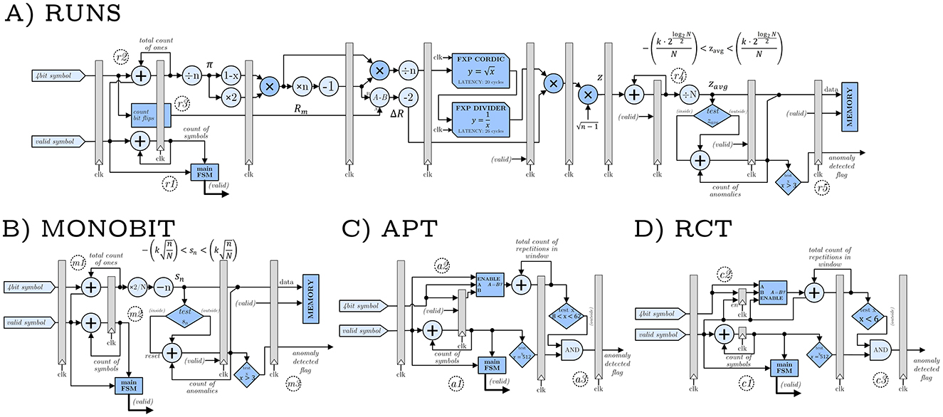
Figure 15. Block diagrams of the hardware-implemented statistical tests. Each accelerator is realized as a Finite-State Machine with Datapath. The (A) RUNS accelerator is the most complex one, since the result depends not only on the parameters but also on the current tested bits, which makes it unfeasible to use pre-calculated values in every step. The (B) Monobit accelerator, thanks to its simpler test statistic, does not suffer from these drawbacks. The (C) APT and (D) RCT accelerators are by far the simplest ones, requiring only counting operations and comparison to predefined thresholds. For the RUNS and Monobit tests, the standard NIST implementation computes a p-value using the error function (erfc). In our hardware implementation, this step is omitted. Instead, the raw test statistics are directly compared against σ-based thresholds derived from the Gaussian approximation of the expected distribution. Consequently, the test reduces to verifying whether the statistic lies within ±kσ, where k determines the confidence level, corresponding to the same acceptance region that would be obtained from the erfc-based p-value.

To improve computational performance and reduce FPGA resource usage, floating-point arithmetic was replaced with fixed-point arithmetic. Fixed-point operations are inherently more efficient for FPGA implementations as they require less logic (and thus lower power consumption), are easier to pipeline, and simplify algorithm integration.

The main contribution of this implementation is the focus on monitoring shifts in the mean of the failure distribution, as explained in Section 6. This adjustment reduces computational overhead while better supporting the goal of identifying distribution drift rather than extreme deviations.

To implement this approach, the system detects three consecutive failures (adjustable from 1 to 16). Assuming these failures are uncorrelated and with a 3σ confidence threshold (0.001 false positive rate), the probability is P = 10⁻⁹. At a 32 Mbit/s generation rate and 64 kbits per test iteration, this corresponds to one false alarm every 69 days on average.

Regarding resource usage, the APT and RCT implementations collectively require approximately 300 Look-Up Table (LUT) elements (0.3% of K26's available resources), 90 registers(< 0.1%), and three block RAM units (2.1%). The Monobit utilizes 480 LUTs (0.4%), 260 registers (0.1%), and 1 block RAM unit (0.7%). Comparatively, the RUNS implementation demands significantly higher resources, using 1,730 LUTs (1.5%), 1,900 registers (0.8%), and three block RAM units (2.1%).

7.1 RUNS test

The FSM controlling the RUNS test operates by processing incoming bit sequences and monitoring their statistical properties in real time. The system is configured with two key parameters: the sequence length n and the number of sequences to analyze N.

During operation, the FSM analyzes each bit sequence through several steps. In reference to Figure 15A, block (r1) counts the incoming symbols by counting the number of clock cycles during which the symbol bus is valid, while block (r2) accumulates the number of ones in each sequence by summing 4 bits from the symbol bus, and block (r3) calculates the number of runs by detecting transitions between consecutive bits. This operation is executed by a module the calculates the number of bit flips in a single symbol. It also remembers the last bit to account for a possible flip between consecutive symbols. These measurements are then used to compute a standardized test statistic z, according to Equation 11, which quantifies how much the observed pattern deviates from expected random behavior.

Among the NIST statistical tests, Monobit, APT, and RCT are easily adapted to firmware as they are based on bit or symbol counting. However, the RUNS test requires complex mathematical operations to compute the normalized z value, as the quantities needed for its evaluation vary with each sequence. This prevents the use of pre-calculated constants and significantly increases computational complexity for firmware implementation.

As a result, two dedicated Xilinx IP cores were used as firmware accelerators: fixed-point CORDIC to calculate the square root of a variable using iterative shift and add/subtract operations, and fixed-point divider (Xilinx Divider generator) to compute the inverse of a variable using the iterative high radix division algorithm. Both accelerators introduce processing latency but offer predictable execution times.

The division operations are performed by simple bit shifting. This is the reason why input parameters (in terms of n and N) were carefully limited. Multiplying by parameters is performed by simple bit shifting operations. Multiplications that involve unpredictable operands (symbolized by darkened circles) are performed by Lookup Tables. Carefully placed result latching regions separate pipeline stages and decrease synthesis and implementation timing requirements.

Block (r4) maintains a running average of these z values, while block (r5) continuously compares them against configurable statistical thresholds. When three consecutive measurements fall outside the acceptable range, the system triggers an anomaly detection flag, allowing external control systems to respond by halting data generation and alerting the administrators.

The implementation supports a flexible configuration for different sequence lengths, ranging from 2⁵ to 2¹¹ bits, and can analyze between 4 and over 2 million sequences, providing adaptability for different testing requirements and performance constraints.

7.2 Monobit test

The implementation of the Monobit test on firmware follows a similar pipeline to the RUNS. Block (m1) counts the number of ones in each generated symbol.

The Monobit test FSM operates in a similar way to the RUNS pipeline. The system processes sequences using the same configurable parameters: sequence length n and number of sequences N.

During execution, block (m1) counts the number of ones in each incoming symbol sequence, while block (m2) controls the FSM execution steps based on symbol reception events. The logic constantly calculates the Sn value, but it is treated as valid only when the required number of bits has been processed, which is typical for FPGA logic designs. The system then computes the average bias across all sequences according to Equation 1, which measures how far the proportion of ones deviates from the expected value. Block (m3) compares these computed averages against predefined statistical thresholds expressed as multiples of standard deviations. The system tracks consecutive threshold violations and raises a hardware failure flag when three consecutive measurements exceed the threshold, indicating potential bias in the generation process.

Raw results, as well as summary statistics, are buffered in FIFO memory for access by other firmware components. Similar to the RUNS, the implementation supports sequence lengths from 2² to 2¹¹ bits and can analyze between 4 and over 2 million sequences, with the constraint that both parameters should have matching parity (both even or both odd powers) to maintain even thresholds and simplify computational operations.

7.3 Adaptive proportion test

The adaptive proportion test (APT) FSM monitors sequences for excessive repetitions of symbols that could indicate biased bit generation. The system operates on fixed-length sequences of 512 symbols to detect statistical anomalies, as recommended by NIST (Turan et al., 2018).

During operation, block (a1) locks the first symbol of each sequence as a reference. Block (a2) then systematically compares each of the following 511 symbols against this locked reference, incrementing an internal counter whenever a match is detected. This process continues until the complete 512-symbol sequence has been analyzed. Upon completion of each sequence, block (a3) evaluates whether the total count of matching symbols exceeds the predetermined statistical threshold. When the count falls outside acceptable boundaries, the system asserts an anomaly flag, signaling potential bias toward a particular symbol value that could compromise randomness quality.

It is worth noting that the counter is reset to one because the first occurrence should also be counted.

7.4 Repetition count test

The repetition count test (RCT) FSM continuously monitors the bit stream for excessive consecutive repetitions of identical symbols, similarly to the RUNS but operated at the symbol level.

During operation, block (c1) processes each incoming symbol in the data stream. Block (c2) maintains a one-cycle delay register that enables comparison between consecutive symbols by storing the previous symbol value. The system then compares the current symbol against the delayed previous symbol, incrementing an internal repetition counter when consecutive matches are detected.

The counter resets to one whenever consecutive symbols differ, ensuring accurate tracking of only continuous repetition sequences. Additionally, the counter undergoes a forced reset after every 512 symbols to remain consistent with NIST specifications.

Block (c3) provides immediate anomaly detection by continuously monitoring the repetition counter against a configurable threshold. When consecutive repetitions exceed the specified limit, the system immediately raises an anomaly flag without waiting for sequence completion.

8 Conclusion

Starting from four wellknown and recognized tests (the Monobit, the RUNS, the repetition count test, and the adaptive proportion test) for the assessment of the eligibility of a string of random bits to seed a DRBG, a method for the online evaluation of the source of randomness is developed. While originally every failing sequence was discarded, here such results are considered in a statistical framework to distinguish between the effect of an actual systematic bias in the bit generation and extreme values that are compatible with ordinary statistical fluctuations.

The sensitivity and effectiveness of bit-wise tests are assessed by introducing a bias model by deliberately forcing the value of some of the bits in the test sequences. On series of 2⁵ sequences of 32 bits, the Monobit-like test is able to identify the tampering of a single bit done once every 10 sequences with a 99.7% confidence level and can go up to spotting a bias once every 100 sequences if the bits forced are in groups of 5. On series of 2¹⁷ sequences of 32 bits, the RUNS-like test is able to pinpoint the presence of a biased bit in 10 sequences with a 5σ confidence level.

The symbol-wise tests, based on the RCT and the APT, are used to provide an online estimation of the entropy of the bit stream. Four different boards implementing our QRNG are evaluated, yielding consistent lower bounds of 3.989 and 3.983 at 3σ for four-bit symbols. Such results are compatible with the calculation of the min-entropy carried out on the boards according to NIST specifications described in (Turan et al. 2018). As this calculation relies on the symbols of the bitstream being independently and identically distributed, the dataset under study was validated as such and the procedure to do so analyzed. While the official procedure does certainly result in a more precise assessment, this method has the advantage of providing an early-stage, online evaluation of a lower bound for the entropy of the random bit generator without any additional burden, as the data used are those provided for the health test.

For all the tests, the concept of inter-sequence failure number (ISN) is introduced and used to evaluate the performance of our QRNG on a statistical basis. As the nature of this observable requires a significant amount of data (much more than the anomaly detection procedure developed on the Monobit and RUNS tests), the tests are implemented in firmware to minimize the lag on bit-harvesting.

The procedures presented in this work, while effective, are subject to several limitations. First, the analysis assumes that the generated data are representative of typical operating conditions; environmental stress tests (temperature extremes, voltage variations) were not performed. As a result, the stability of the proposed methods under such conditions remains to be assessed. Second, the choice of thresholds (e.g., 3σ, α = 2⁻²⁰) reflects a balance between sensitivity and false-alarm probability. These values, although consistent with NIST recommendations, retain a degree of heuristic tuning and could require re-optimization for alternative use cases. However, this flexibility can be considered a strength of the proposed methodology, as these values can be adjusted by the user depending on the sensitivity, false positive rate, and reaction time required by the specific application.

Finally, we remark that the proposed tests yield significant results starting from a relatively small sample of generated bits. This opens the way for highly optimized implementations of entire test suites using FPGAs, which would enable a resource-efficient randomness assessment of generated bit-streams without significantly slowing down the harvesting process.

Data availability statement

The datasets presented in this article are not readily available because datasets were binary files of random bits generated with a TRNG. Requests to access the datasets should be directed to Massimo Caccia, bWFzc2ltby5jYWNjaWFAcmFuZG9tcG93ZXIuZXU=.

Author contributions

CC: Data curation, Formal analysis, Investigation, Software, Visualization, Writing – original draft, Writing – review & editing. VR: Data curation, Formal analysis, Investigation, Software, Visualization, Writing – original draft, Writing – review & editing. KW: Data curation, Investigation, Software, Visualization, Writing – original draft, Writing – review & editing. AT: Project administration, Supervision, Validation, Writing – review & editing. MB: Resources, Writing – review & editing. PD: Resources, Writing – review & editing. WK: Project administration, Supervision, Resources, Writing – review & editing. MC: Conceptualization, Formal analysis, Funding acquisition, Investigation, Methodology, Project administration, Supervision, Validation, Writing – review & editing.

Funding

The author(s) declare that financial support was received for the research and/or publication of this article. This activity is part of the project named In-silico quantum generation of random bit streams (Random Power) which has received funding from the European Union's Horizon 2020 Research and Innovation Programme within the ATTRACT cascade grant project, under the contract no.101004462). The European Commission' support does not constitute an endorsement of the contents, which only reflect the views of the authors. The Commission is not responsible for any use of the information therein.

Acknowledgments

The authors would like to thank Filippo Bonazzi, Olivia Riccomi, and Matteo Huang for their contribution to the implementation of the IID procedure and analysis.²

Conflict of interest

CC, VR, KW, MB, and MC were employed by Random Power s.r.l.

The remaining authors declare that the research was conducted in the absence of any commercial or financial relationships that could be construed as a potential conflict of interest.

Generative AI statement

The author(s) declare that no Gen AI was used in the creation of this manuscript.

Any alternative text (alt text) provided alongside figures in this article has been generated by Frontiers with the support of artificial intelligence and reasonable efforts have been made to ensure accuracy, including review by the authors wherever possible. If you identify any issues, please contact us.

Publisher's note

All claims expressed in this article are solely those of the authors and do not necessarily represent those of their affiliated organizations, or those of the publisher, the editors and the reviewers. Any product that may be evaluated in this article, or claim that may be made by its manufacturer, is not guaranteed or endorsed by the publisher.

Footnotes

1. ^https://github.com/RandomPower/IID_validations

2. ^https://github.com/RandomPower/IID_validation

References

Barker, E., and Kelsey, J. (2015). Recommendation for Random Number Generation Using Deterministic Random Bit Generators. Gaithersburg, MD: National Institute of Standards and Technology. doi: 10.6028/NIST.SP.800-90Ar1

Crossref Full Text | Google Scholar

Barker, E., Kelsey, J., McKay, K., Roginsky, A., and Sönmez Turan, M. (2012). Recommendation for Random Bit Generator (RBG) Constructions. Gaithersburg, MD: NIST special publication. U.S. Department of Commerce, National Institute of Standards and Technology.

Google Scholar

Bradley, J. V. (1968). Distribution-Free Statistical Tests. Englewood Cliffs, NJ: Prentice-Hall, 283–310.

Google Scholar

Caccia, M., Malinverno, L., Paolucci, L., Corridori, C., Proserpio, E., Abba, A., et al. (2020). In-silico generation of random bit streams. Nucl. Instrum. Methods Phys. Res. A 980:164480. doi: 10.1016/j.nima.2020.164480

Crossref Full Text | Google Scholar

Caratozzolo, C., Rossi, V., Witek, K., Trombetta, A., and Caccia, M. (2024). “On-line anomaly detection and qualification of random bit streams,” in 2024 IEEE International Conference on Cyber Security and Resilience (CSR) (London: IEEE), 897–904. doi: 10.1109/CSR61664.2024.10679431

Crossref Full Text | Google Scholar

Cowan, G. (2016). “Review of particle physics, 2016-2017,” in The Monte Carlo Techniques. Particle Data Group, 537. Available online at: https://cds.cern.ch/record/2241948/files/openaccess_cpc_40_10_100001.pdf

Google Scholar

Debian Security Team (2008). [DSA 1571-1] New Openssl Packages Fix Predictable Random Number Generator. Debian Security Advisory. Available online at: https://lists.debian.org/debian-security-announce/2008/msg00152.html

Google Scholar

Fagan, M., Megas, K. N., Cuthill, B., Marron, J., and Hoehn, B. (2025). Foundational Cybersecurity Activities for IOT Product Manufacturers. Gaithersburg, MD: NIST Internal Report NISTIR 8259r1 ipd, National Institute of Standards and Technology. Initial Public Draft.

Google Scholar

Feng, Y., and Hao, L. (2020). Testing randomness using artificial neural network. IEEE Access 8, 163685–163693. doi: 10.1109/ACCESS.2020.3022098

Crossref Full Text | Google Scholar

Figotin, A., Vitebskiy, I., Popovich, V., Stetsenko, G., Molchanov, S., Gordon, A., et al. (2004). Random Number Generator Based on the Spontaneous Alpha-Decay. US Patent 6,745,217.

Google Scholar

Foreman, C., Yeung, R., and Curchod, F. J. (2024). Statistical testing of random number generators and their improvement using randomness extraction. Entropy 26:1053. doi: 10.3390/e26121053

PubMed Abstract | Crossref Full Text | Google Scholar

Fox, B. (2021). You're Doing IoT RNG: The Crack in the Foundation of IoT. Blog Post. Available online at: https://bishopfox.com/blog/youre-doing-iot-rng

Google Scholar

Frustaci, F., Spagnolo, F., Corsonello, P., and Perri, S. (2024). A high-speed and low-power dsp-based trng for fpga implementations. IEEE Trans. Circuits Syst. II: Express Briefs 71, 4964–4968. doi: 10.1109/TCSII.2024.3421323

Crossref Full Text | Google Scholar

Gennaro, R. (2006). Randomness in cryptography. Secur. Privacy IEEE 4, 64–67. doi: 10.1109/MSP.2006.49

Crossref Full Text | Google Scholar

Goel, R., Xiao, Y., and Ramezani, R. (2024). “Transformer models as an efficient replacement for statistical test suites to evaluate the quality of random numbers,” in 2024 International Symposium on Networks, Computers and Communications (ISNCC) (Washington DC: IEEE), 1–6. doi: 10.1109/ISNCC62547.2024.10758985

Crossref Full Text | Google Scholar

Haitz, R. H. (1965). Mechanism contributing to the noise pulse rate of avalanche diodes. J. Appl. Phys. 36, 3123–3131. doi: 10.1063/1.1702936

Crossref Full Text | Google Scholar

Herrero-Collantes, M., and Garcia-Escartin, J. C. (2017). Quantum random number generators. Rev. Mod. Phys. 89:015004. doi: 10.1103/RevModPhys.89.015004

Crossref Full Text | Google Scholar

L'Ecuyer, P., and Simard, R. J. (2007). Testu01: a C library for empirical testing of random number generators. ACM Trans. Math. Softw. 33, 22:1–22.40. doi: 10.1145/1268776.1268777

Crossref Full Text | Google Scholar

Lu, Y., Xu, E., Liu, Y., Chen, J., Liang, H., Huang, Z., et al. (2025). Ultra-high efficiency trng ip based on mesh topology of coupled-xor. IEEE Trans. Circuits Syst. I: Regul. Pap. 72, 2754–2767. doi: 10.1109/TCSI.2025.3555325

Crossref Full Text | Google Scholar

McKay, K. G. (1954). Avalanche breakdown in silicon. Phys. Rev. 94, 877–884. doi: 10.1103/PhysRev.94.877

Crossref Full Text | Google Scholar

Piscopo, V., Dolmeta, A., Mirigaldi, M., Martina, M., and Masera, G. (2025). A high-entropy true random number generator with parameterizable architecture on fpga. Sensors 25:1678. doi: 10.3390/s25061678

PubMed Abstract | Crossref Full Text | Google Scholar

Rukhin, A., Soto, J., Nechvatal, J., Smid, M., and Barker, E. (2001). A Statistical Test Suite for Random and Pseudorandom Number Generators for Cryptographic Applications. Gaithersburg, MD: NIST Special Publication 800-22, 163. doi: 10.6028/NIST.SP.800-22

Crossref Full Text | Google Scholar

Senitzki, B. M. J. (1958). Breakdown in silicon. Phys. Rev. 110, 612–620. doi: 10.1103/PhysRev.110.612

Crossref Full Text | Google Scholar

Seyhan, K., and Akleylek, S. (2022). Classification of random number generator applications in IOT: a comprehensive taxonomy. J. Inf. Secur. Appl. 71:103365. doi: 10.1016/j.jisa.2022.103365

Crossref Full Text | Google Scholar

Soto, J., and Bassham, L. (2000). Randomness Testing of the Advanced Encryption Standard Finalist Candidates. Gaithersburg, MD: NIST. doi: 10.6028/NIST.IR.6483

Crossref Full Text | Google Scholar

Sýs, M., Klinec, D., and Svenda, P. (2017). “The efficient randomness testing using boolean functions,” in Proceedings of the 14th International Joint Conference on e-Business and Telecommunications (ICETE 2017) - Volume 4: SECRYPT, Madrid, Spain, July 24-26, 2017, eds. P. Samarati, M. S. Obaidat, and E. Cabello (Setúbal: SciTePress), 92–103. doi: 10.5220/0006425100920103

Crossref Full Text | Google Scholar

Turan, M., Barker, E., Kelsey, J., McKay, K. A., Baish, M. L., and Boyle, M. (2018). Recommendation for the Entropy Sources Used for Random Bit Generation. Gaithersburg, MD: National Institute of Standards and Technology. 84. doi: 10.6028/NIST.SP.800-90B

PubMed Abstract | Crossref Full Text | Google Scholar

Wu, S. (2025). Lightweight high-throughput true random number generator via state-switchable ring oscillators. J. Syst. Archit. 100:02305 doi: 10.1016/j.vlsi.2024.102305

Crossref Full Text | Google Scholar

Yilek, S., Rescorla, E., Shacham, H., Enright, B., and Savage, S. (2009). “When private keys are public: results from the 2008 debian openssl vulnerability,” in Proceedings of the 9th ACM SIGCOMM Internet Measurement Conference, IMC 2009, Chicago, Illinois, USA, November 4-6, 2009, eds. A. Feldmann and L. Mathy (New York, NY: ACM), 15–27. doi: 10.1145/1644893.1644896

Crossref Full Text | Google Scholar

Zhang, B., Li, L., Xu, Y., Tan, X., Shi, J., Huang, P., et al. (2025). Practical attack on a quantum random number generator via classical fluctuations. Phys. Rev. Appl. 24:014008. doi: 10.1103/k3c9-ngt1

Crossref Full Text | Google Scholar

Zhang, Y., Zhong, K., and Zhong, J. (2025). Dh-trng: dynamic hybrid true random number generator for ultra-high throughput and energy efficiency. arXiv [preprint]. arXiv:2502.01066. doi: 10.48550/arXiv.2502.01066

Crossref Full Text | Google Scholar