 Carlos Augusto Musetti de Assis1,2,3*
 Luana Queiroz Pinho1,2
 Alexandre Macedo Fernandes1
 Moacyr Araujo2,4,5
 Leticia Cotrim da Cunha1,2,5
- 1Programa de Pós-Graduação em Oceanografia, Laboratório de Oceanografia Química, Universidade do Estado do Rio de Janeiro (UERJ), Rio de Janeiro, RJ, Brazil
- 2Brazilian Ocean Acidification Network (BrOA), Universidade Federal do Rio Grande (FURG), Rio Grande, RS, Brazil
- 3GEOMAR Helmholtz Centre for Ocean Research Kiel, Kiel, Germany
- 4Departamento de Oceanografia, DOCEAN/Universidade federal de Pernambuco (UFPE), Recife, Brazil
- 5Brazilian Research Network on Global Climate Change (Rede CLIMA), São José dos Campos, SP, Brazil
The Western Tropical Atlantic Ocean (WTAO) is crucial for understanding CO2 dynamics due to inputs from major rivers (Amazon and Orinoco), substantial rainfall from the Intertropical Convergence Zone (ITCZ), and CO2-rich waters from equatorial upwelling. This study, spanning 1998 to 2018, utilized sea surface temperature (SST) and sea surface salinity (SSS) data from the PIRATA buoy at 8°N 38°W to reconstruct the surface marine carbonate system. Empirical models derived total alkalinity (TA) and dissolved inorganic carbon (DIC) from SSS, with subsequent estimation of pH and fCO2 from TA, DIC, SSS, and SST data. Linear trend analysis showed statistically significant temporal trends: DIC and fCO2 increased at a rate of 0.7 µmol kg-1 year-1 and 1.539 µatm year-1, respectively, and pH decreased at a rate of -0.001 pH units year-1, although DIC did not show any trend after data was de-seasoned. Rainfall analysis revealed distinct dry (July to December) and wet (January to June) seasons, aligning with lower and higher freshwater influence on the ocean surface, respectively. TA, DIC, and pH correlated positively with SSS, exhibiting higher values during the dry season and lower values during the wet season. Conversely, fCO2 correlated positively with SST, showcasing higher values during the wet season and lower values during the dry season. This emphasizes the influential roles of SSS and SST variability in CO2 solubility within the region. Finally, we have analysed the difference between TA and DIC (TA-DIC) as an indicator for ocean acidification and found a decreasing trend of -0.93 ± 0.02 μmol kg-1 year-1, reinforcing the reduction in the surface ocean buffering capacity in this area. All trends found for the region agree with data from other stations in the tropical and subtropical Atlantic Ocean. In conclusion, the use of empirical models proposed in this study has proven to help filling the gaps in marine carbonate system data in the Western Tropical Atlantic.
1 Introduction
With the advance of human civilization in the past decades came the increase of carbon dioxide (CO2) emissions in the atmosphere due to the burning of fossil fuels, the main present source of energy (Mardani et al., 2019). This is one of the greenhouse gases responsible for keeping the global temperature steady. Nonetheless, the rise of CO2 emissions has been leading to global changes such as global atmosphere and ocean warming, a decrease in seawater pH, as well as an increase of extreme climatic events’ frequency (Allen et al., 2009; Doney et al., 2009; Baker et al., 2018).
The global ocean serves as a significant CO2 sink, absorbing approximately 25% of annual human emissions (Sabine et al., 2004; Friedlingstein et al., 2022). Carbon dioxide’s solubility at the sea surface depends primarily on sea surface temperature (SST) and sea surface salinity (SSS), rendering the global ocean a complex, dynamic system intricately linked to the atmosphere (Goodwin and Lenton, 2009; Takahashi et al., 2009; Merlivat et al., 2015). When CO2 reacts with water, it forms carbonic acid (H2CO3), releasing protons (H+) and bicarbonate ions (HCO3-). The increase in the CO2 absorption results in a reduction of carbonate saturation, effect known as ocean acidification, affecting organisms with calcified structures, as illustrated in Equation 1 (Guinotte and Fabry, 2008; Pörtner, 2008; Kroeker et al., 2010; Mangi et al., 2018; Bednaršek et al., 2019). This phenomenon has various impacts on marine life, including hindering the formation of calcareous structures, reducing recruitment rates of organisms on coral reefs, and intensifying competition between non-calcifying and calcifying organisms (Bignami et al., 2013; Allen et al., 2017).
Biological processes significantly influence CO2 dynamics in the ocean. Intense primary production consumes dissolved CO2, elevating seawater pH. Conversely, when respiration surpasses primary production, CO2 is added to the water, causing a pH decline (Sunda and Cai, 2012; Buapet et al., 2013). Notably, this impact is more pronounced in coastal regions and oceanic areas experiencing intense upwelling (Dugdale et al., 2002; McGillis et al., 2004; Wallace et al., 2014).
The reactions involve essential components of the marine carbonate system: total alkalinity (TA), dissolved inorganic carbon (DIC), pH, and CO2 fugacity (fCO2). TA represents the surplus of proton acceptor species in seawater, primarily carbonate and bicarbonate ions at a pH of 8.1. Contributions from the boric system and water dissociation components are considered (Dickson, 1981; Wolf-Gladrow et al., 2007; Emerson and Hedges, 2008; Doney et al., 2009).
DIC comprises dissolved CO2, carbonic acid (H2CO3), bicarbonate, and carbonate ions, representing the summation of all inorganic carbon species in seawater (Emerson and Hedges, 2008). The pH scale measures seawater acidity and can be represented in various scales, defined as the negative logarithm (base 10) of the H+ ion concentration, indicating water acidity levels (Marion et al., 2011). fCO2 corrects the partial pressure of CO2 (pCO2) from an ideal to a real gas, representing the gas pressure exerted within the water (Dickson et al., 2007).
Any two of the marine carbonate system parameters, together with SSS and sea surface temperature (SST) values, can be used to calculate the remaining parameters (Schneider et al., 2007; Fassbender et al., 2017). Empirical models correlating TA and DIC with sea surface salinity (SSS) have a great importance in comprehending the marine carbonate system as they can be used in historic series for reconstructing past data (Lee et al., 2006; Lefévre et al., 2010; Bonou et al., 2016). Most of the carbonate system parameters of this system were not usually measured in the past, meaning that calculating them from SSS data is a good alternative when these empirical models are well established for the study area.
The tropical Atlantic (30°S-30°N; 80°W-20°E) acts on average as a source of CO2 to the atmosphere, mainly because of higher temperatures decreasing the gas solubility, as well as the equatorial upwelling bringing CO2-rich subsurface water and increasing the CO2 fugacity at the ocean surface (Takahashi et al., 2009; Schuster et al., 2013). However, the Western Tropical Atlantic Ocean (WTA) goes the other way around, becoming a large sink of atmospheric CO2 at the Tropical Atlantic from July to December, in response to large inputs of freshwater, both from the Intertropical Convergence Zone’s (ITCZ) rainfall and from the Amazon River plume. During that period, Amazon waters widely spread to the western parts of the WTA after the North Brazilian Current (NBC) retroflection and eastward transport by North Equatorial Countercurrent (NECC) (Mitchell and Wallace, 1992; Körtzinger, 2003; Bruto et al., 2017; Lefèvre et al., 2017).
Time series are of great importance in the study of trends and variability in the marine carbonate system. Bates et al. (2014) observed a trend in DIC, pH, pCO2 and other parameters in this system from time series with 15 to 30 years in five stations in the Atlantic Ocean and two stations in the Pacific, elucidating how different parts of the global ocean responded to the increase in atmospheric concentrations of CO2, as well as to ocean acidification.
The PIRATA project, initiated in 1997, aims to understand Tropical Atlantic Ocean variability. Using 18 moored buoys, it forms a real-time observation network to monitor meteorological and oceanographic variables (Bourlès et al., 2019; Foltz et al., 2019). This multinational effort enhances our ability to predict ocean-atmosphere variability. Moored buoys are crucial for capturing temporal variations in oceanographic parameters in the open ocean (Lefèvre et al., 2008; Bruto et al., 2017). Bruto et al. (2017) used the time series of hourly surface ocean fCO2 data from the PIRATA buoy at 8° N 38° W, the same used in this study, from 2008 to 2011, where it was observed that, in addition to two distinct seasonal periods, fCO2 also showed a high-frequency variation (less than 24h) associated with the daily cycle of solar radiation and heavy rainfall.
The WTA has been the focus of studies about the carbon cycle because of its great complexity and global importance concerning CO2 dynamics (Araujo et al., 2017; Bonou et al., 2022, 2016; Lefèvre et al., 2017; de Carvalho-Borges et al., 2018; Monteiro et al., 2022). Although many studies show the spatial variation of the carbonate system on the WTA and its relationship with the Amazon River plume, few studies focus on analyzing its variation over longer periods of time from in situ observations. This study used a time series from 1998 to 2018 of SSS and SST data from the PIRATA buoy at 8° N 38° W and calculated the carbonate system parameters (TA, DIC, pH and fCO2) to detect these parameters’ variation with time in a region with complex CO2 dynamics.
2 Materials and methods
2.1 Data
The “Prediction and Research moored Array in the Tropical Atlantic” (PIRATA) project consists of an in-situ observation network composed of 18 moored buoys judiciously spread in the Tropical Atlantic. These include five buoys located along the 38°W meridian (4°N, 8°N, 12°N, 15°N, and 20°N). Each of these buoys are equipped with meteorological sensors to measure the direction and speed of the wind at 4 meters height, air temperature, rain rate, relative humidity and short-wave solar radiation. Temperature sensors are positioned beneath the ocean surface at depths of 1, 20, 40, 80, 120, 180, 300, and 500 meters, collecting measurements every 10 minutes. Salinity sensors are also deployed at depths of 1, 20, 40, and 120 meters, recording hourly measurements. The 8°N 38°W buoy data was considered in our study because: (i) it represents the PIRATA site under the strong seasonal influence of the Amazon River plume waters transported eastward by NECC and rainfall from the ITCZ; and (ii) a CARbon Interface Ocean Atmosphere (CARIOCA) sensor was installed on that mooring line from 2008–2013, registering in situ seawater fCO2 hourly values (Bruto et al., 2017). For this study, SSS and SST, both at 1m depth, and rain rate data from the buoy located at 8°N 38°W were used (Figure 1) with a total of 3789 SSS and 5669 SST data. The daily averaged sea surface temperature (SST) and sea surface salinity (SSS) values are transmitted in real time by the Global Telecommunication System (GTS) and are freely available at PIRATA sites (e.g., http://www.pmel.noaa.gov/pirata) (Supplementary Material 1).
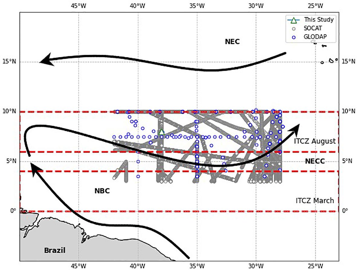
Figure 1 Study area. The green triangle represents the PIRATA mooring site at 8°N 38°W used in this study. The blue dots illustrate points where TA, DIC and pH data from GLODAPv2.2022 were used. The main surface currents are also shown on the map, together with the mean position of the Intertropical Convergence Zone (ITCZ) at its southernmost (March) and northernmost (August) months. NEC, North Equatorial Current; NECC, North Equatorial Countercurrent; NBC, North Brazilian Current.
The SST and SSS data used in this study, from 1998 to 2018, were measured by the following sensors: a thermistor model 46006 from Yellow Springs Instruments (YSI) for measuring SST, with resolution of 0.001°C, range from 14 to 32°C and accuracy of ± 0.03°C (A’Hearn et al., 2002; Freitag et al., 2005), and, for the measurement of SSS, internal field conductivity cell of model SBE16 (Seacat) from Sea Bird Electronics with 0.0001 S m-1 resolution, range from 3 to 6 S m-1 and accuracy of ± 0.02 psu (Freitag et al., 1999). The lack of SSS data in relation to SST in the PIRATA buoy at 8°N 38°W is especially striking in the period from 2003 to 2008. As of 2010, both the available SSS and SST data decreased considerably due to vandalism and problems with the buoy’s operation and maintenance. The rain rate data used to differentiate the two seasons in the time series were measured by a capacitance sensor from R. M. Young, model 50203–34, with resolution of 0.2 mm h-1, range from 0 to 50 mm and accuracy of ± 0.4 mm h-1 on 10 min filtered data (Serra et al., 2001). The PIRATA project conducts annual cruises dedicated to the retrieval of buoys and the maintenance of equipment. These cruises are essential for ensuring the continued functionality and reliability of the project’s monitoring infrastructure. The data used in this study followed the World Ocean Circulation Experiment (WOCE) quality flag system (Gouretski and Koltermann, 2004), using Quality Flag (QF) 2 for valid data and 5 for missing data.
2.2 Calculation of parameters
In this study, the calculation of TA relied on the equation proposed by Lefévre et al. (2010) (Equation 2), which correlates TA with SSS in the Western Tropical Atlantic. It’s important to note the associated error of 11.6 µmol kg-1 in predicted alkalinity using this equation. Similarly, for DIC, the equation proposed by Bonou et al. (2016) was employed (Equation 3), presenting an error of 24 µmol kg-1 in predicted DIC. Additionally, an annual increase of 0.9 µmol kg-1 in DIC since 1989 was factored in to account for the escalating annual CO2 emissions into the atmosphere. As detailed by Bonou et al. (2016), the inclusion of SST data in these regression equations did not significantly enhance correlation, indicating that SSS variations exerted a more substantial influence on TA and DIC variability in the Western Tropical Atlantic compared to SST. The uncertainties of these estimations were thoroughly discussed by the authors before mentioned, highlighting the importance of regionally using these equations, as they are strongly related to the local SSS variation observed in the WTA.
To reconstruct pH and fCO2 data from SST, SSS, TA, and DIC, the PyCO2SYS package (Version 1.8.2) for Python (Humphreys et al., 2022) was employed. The dissociation constants of carbonic acid in seawater as a function of salinity and temperature defined by Millero et al. (2006) and the KSO4 dissociation constant by Dickson (1990) (Bonou et al., 2016; Monteiro et al., 2022), were utilized. The pH scale used in this study is the total scale (Marion et al., 2011). The total probable errors were estimated by propagation, leading to estimated errors of 0.041and 45.00 µatm, for pH and fCO2, respectively (Millero et al., 2006). While this study exclusively presented results for TA, DIC, fCO2, and pH, the calculated surface ocean CO2 molar fraction (xCO2) and partial pressure (pCO2) values were also.
Since the empirical models used in this paper use only SSS and time to calculate TA and DIC trends along time, these parameters, in addition to pH and fCO2, which were calculated from the before mentioned parameters, follow the same distribution over the years of SSS data. Furthermore, the Anderson-Darling test results showed that all variables involved in this study (SSS, SST, TA, DIC, pH and fCO2) had non-normal distribution (Table 1) (Miot, 2017), although the mean and median values were close to each other.
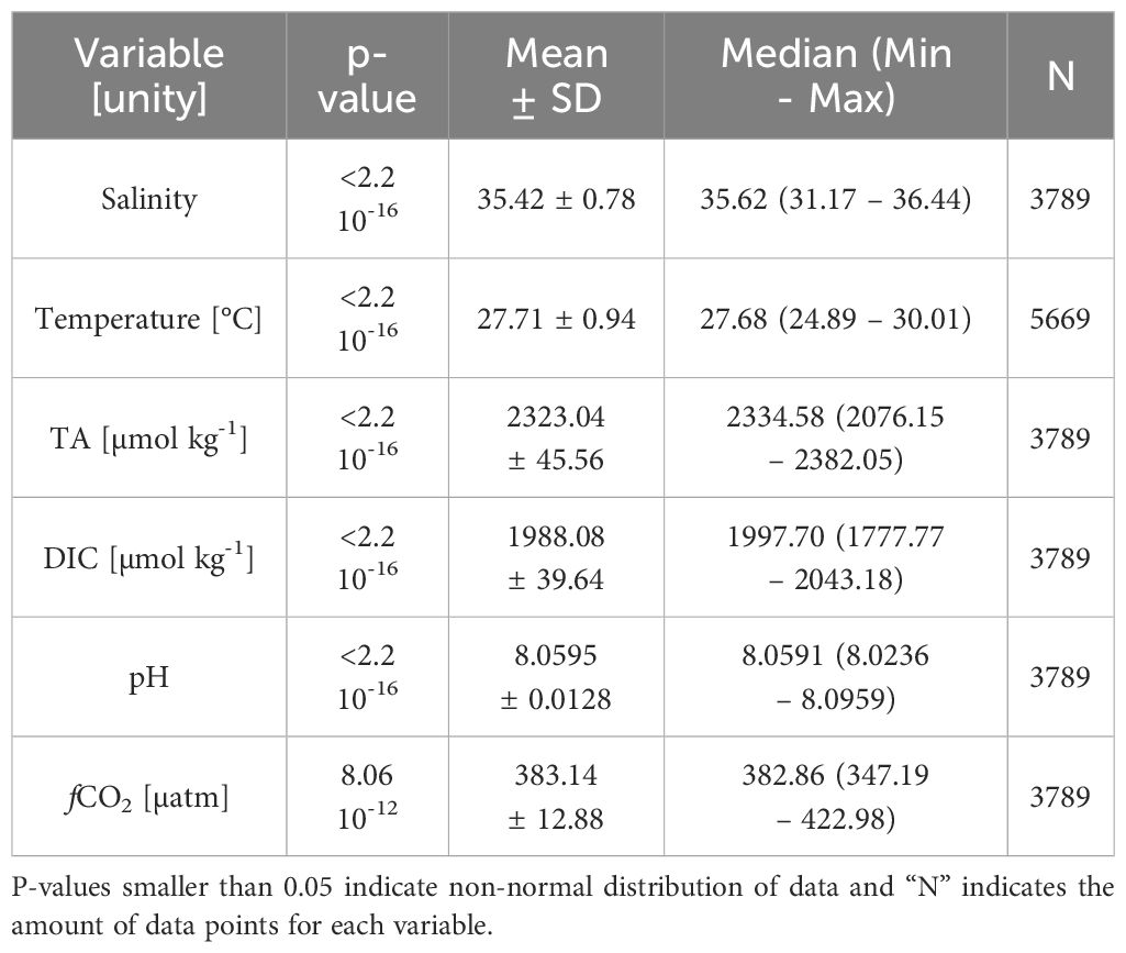
Table 1 p-value of the Anderson-Darling test and measures of central tendency of the data (mean ± standard deviation) and median (minimum and maximum values) for sea surface salinity, temperature, total alkalinity, dissolved inorganic carbon, pH and fCO2.
TA and DIC data were normalized to mean SSS (35,4) according to the following the method described by Friis et al. (2003) (Equation 4).
Where:
nXi = normalized variable at given “i” moment
Xi = variable at given “i” moment (TA or DIC)
XS=0 = variable at 0 salinity
Si = salinity at given “i” moment
Sref = salinity at reference level. At this study we used the mean salinity of our data (35.42)
2.3 Databases for comparison
For this study, data up to 20 m depth of TA, DIC and pH measurements between latitudes 3° and 10° N and longitudes of 28° and 42° W from the GLODAPv2.2022 data product (Global Data Analysis Project) (Lauvset et al., 2022) were used, with a total of 69 TA data, 58 DIC data and 69 pH data (Figure 1). Data corresponds to the period from 1998 to 2018 and a mean depth of 9 m. GLODAP data is publicly available at https://www.glodap.info/. The 20 m depth was estimated based on the estimation of the regional mixed layer depth from De Boyer Montégut et al. (2004). Changes in pressure in the chosen depth do not affect TA data due to its conservative properties (Middelburg et al., 2020).
To compare with the fCO2 data calculated in this study, fCO2 data from the SOCAT platform were used (Bakker et al., 2016). The same area as used for GLODAP was selected and only data from 1998 to 2018 were accepted (totalizing 41212 data). The study also utilized daily averages of hourly fCO2 data from the CARIOCA sensor, installed in the same buoy as a reference (Lefèvre et al., 2008; Merlivat et al., 2015) from 2008 to 2011 to compare with the study’s results and visualize the model’s variation around actual values. Daily averages for fCO2 were preferred due to the use of daily averages of hourly SSS and SST data from the PIRATA buoy in the study. This approach aimed to prevent high-frequency variations in fugacity, observed in the region (Bruto et al., 2017), from affecting the comparison. In situ CO2-related measurements obtained at 8°N 38°W are already included in these global data products. GLODAP and SOCAT data description for these comparisons can be seen in Table 2.
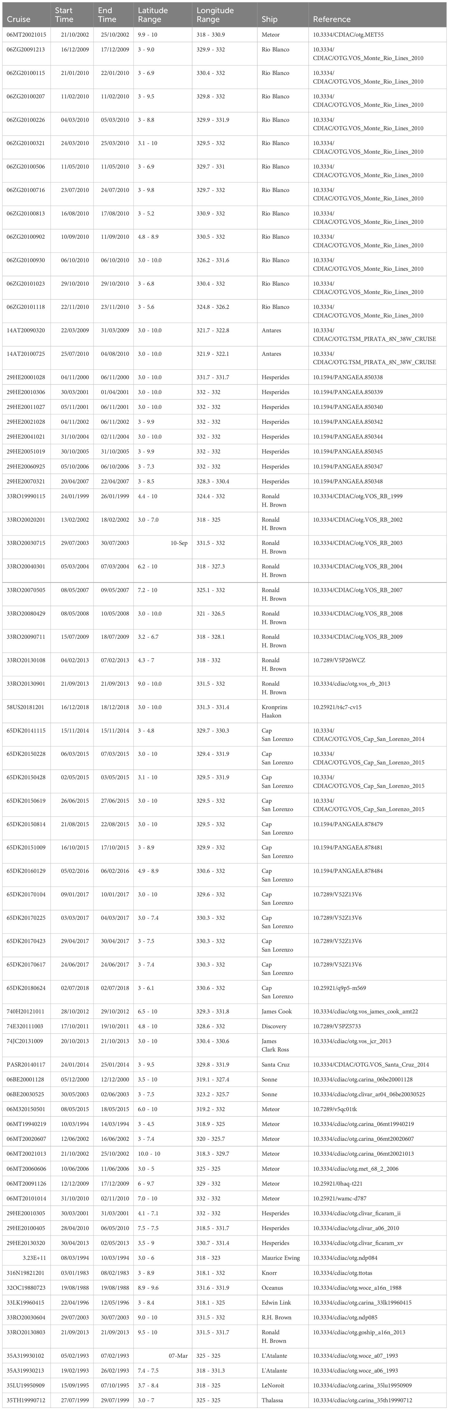
Table 2 Metadata for GLODAP and SOCAT data used in this study.
In order to compare the surface trend with the atmospheric trend of CO2, data from the Ragged Point station, Barbados, 13°N-59°W (http://www.esrl.noaa.gov/gmd/ccgg/iadv/) from NOAA/Earth System Research Laboratory (ESRL) Global Monitoring Division were used, as it is the closest location to the PIRATA 8°N 38°W buoy with measurement of atmospheric CO2 (Figure 2).
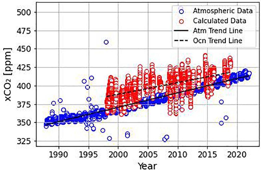
Figure 2 Sea surface CO2 molar fraction data (xCO2) calculated in this study (red circles) and atmospheric xCO2 at Ragged Point station, Barbados (blue square). The dashed line indicates the linear trend on the sea surface calculated in this study, and the full line represents the atmospheric trend based on data from the Ragged Point station.
2.4 Statistical analyses
The Anderson-Darling test was used to check for the normality of our data, as it is more efficient in large databases (Razali and Wah, 2011; Miot, 2017). All variables showed non-normal distribution. To estimate the time trend for the parameters calculated in this study, a linear regression was used, in which the slope indicates the annual variation of the parameter. On the other hand, the method described by Sutton et al. (2022) was used to remove seasonality from data. The method consists of de-seasoning the time series based on monthly climatology anomalies and then calculating the linear regression of the de-seasoned data. This method reduces variability and autocorrelation in environmental datasets (Bates et al., 2014). Although the linear regression is a parametric test, it was used in order to keep an agreement with other time series studies in the field.
To compare the calculated values of TA, DIC and pH with the in-situ data available in GLODAP, as well as the calculated values of fCO2 with the data from SOCAT, the Wilcoxon-Mann-Whitney test was used. This same test was also used to evaluate if the two seasons observed in this study were statistically different. p-values<0.05 reject the null hypothesis, suggesting statistical differences in medians and population divergence.
3 Results
3.1 Seasonality
Based on the monthly variation of rain rate, two characteristic periods were observed (Figure 3): one from July to December with high rainfall (0.67 ± 0.82 mm h-1), here called the wet season, and a period from January to June with lower rates of rainfall (0.23 ± 0.44 mm h-1), here called the dry season. Both seasons showed statistically significant difference through the Mann-Whitney test (rainfall, SSS, SST, TA, DIC, pH and fCO2 presented p-values smaller than 0.05).
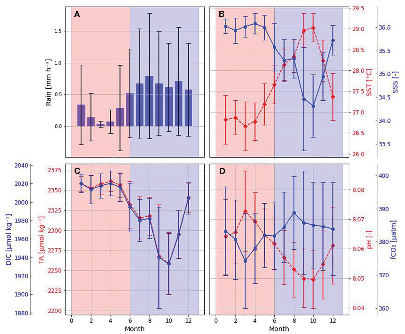
Figure 3 Climatology of observed and estimated parameters at the PIRATA buoy 8°N-38°W based on monthly means. (A) Rain rate (mm h-1); (B) Sea surface salinity (blue dots) and temperature (°C, red dots); (C) Total alkalinity (µmol kg -1, blue dots) and dissolved inorganic carbon (µmol kg -1, red dots); (D) pH (red dots) and CO2 fugacity (fCO2, in µatm, blue dots). The bars at each month at (A–D) indicate the standard deviation. Red shaded areas in the plots represent dry season (January to June) and blue shaded areas, wet season (July to December).
Mean SST varied in a similar way as mean rainfall, with lower values during dry season (26.99 ± 0.50°C) and higher values during wet season (28.34 ± 0.43°C), while mean SSS varied opposite to mean rainfall, with higher values during dry season (35.94 ± 0.27) and lower values during wet season (35.01 ± 0.58). The monthly calculated mean TA and DIC followed the SSS variation, with higher values during dry season, with a mean value of 2352.9± 16.0 µmol kg-1 for TA and 2013.8 ± 15.6 µmol kg-1 for DIC, and lower values during wet season, with a mean value of 2299.2 ± 33.6 µmol kg-1 for TA and 1967.4 ± 29.2 µmol kg-1 for DIC. Calculated pH showed a monthly variation similar to that of salinity, with a standard deviation similar between the two seasons, but higher values during dry season, mean of 8.066 ± 0.011, and lower values during wet season, with a mean value of 8.054 ± 0.010. The observed similarity in pH values, even when considering 2–3 decimal places, warrants discussion regarding potential differences in other variables during these periods. While our study focused on analyzing pH and temperature and salinity variations, it is essential to acknowledge the influence of additional factors such as dissolved oxygen levels, and nutrient concentrations, may have contributed to the observed patterns. Further investigation into these variables could provide insights into the underlying mechanisms driving the observed pH variations between seasons. Calculated surface ocean CO2 fugacity (fCO2), on the other hand, showed the opposite variation in comparison to SSS, with lower values during dry season, mean of 380.0 ± 11.7 µatm, and higher values during wet season, with a mean value of 385.4 ± 12.9 µatm.
3.2 Comparison with other databases
TA, pH and fCO2 had statistically significant differences (p-value< 0.05) (Table 3), with this study underestimating the values (Table 1) when compared to GLODAP (Figure 4) and SOCAT (lower medians) (Figure 5); yet DIC didn’t have statistically significant differences (p-value ≥ 0.05), although it had lower median than the one from GLODAP data. However, when separating the data according to the season (dry and wet), it was possible to observe that, in the dry season, all parameters showed statistically different medians (p-value< 0.05), with the exception of pH. On the other hand, during wet season, only TA showed statistically equal medians (p-value ≥ 0.05), while DIC, pH and fCO2 showed p-values smaller than 0.05.
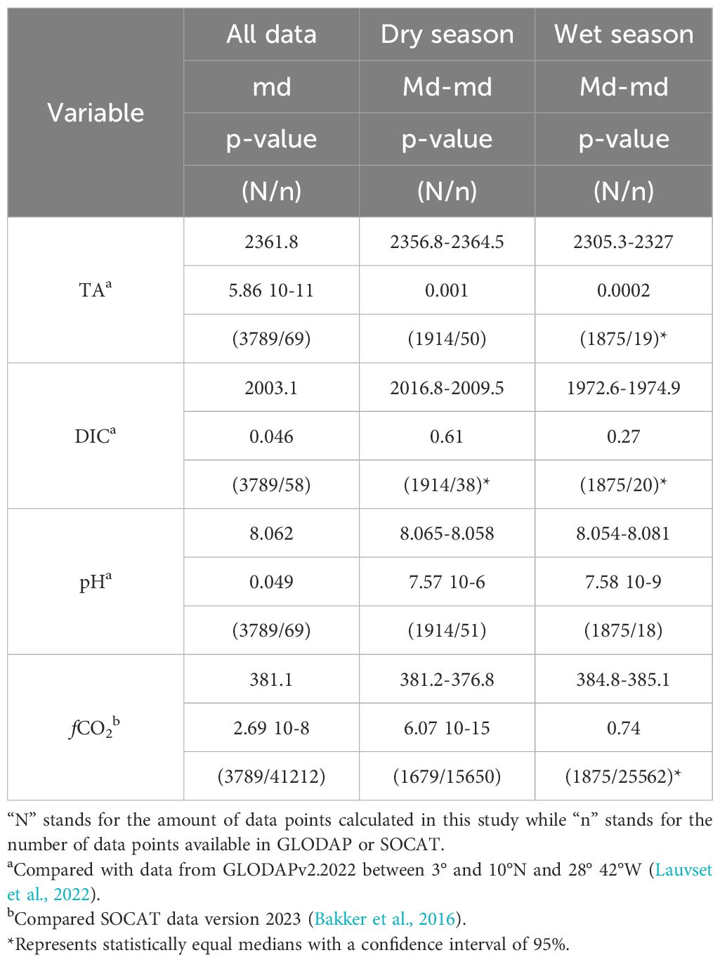
Table 3 Medians (Md – calculated in this study, md – data available in GLODAP or SOCAT) and p-value of the Wilcoxon-Mann-Whitney test for surface total alkalinity (TA, in µmol kg-1), dissolved inorganic carbon (DIC, in in µmol kg-1), pH and CO2 fugacity (fCO2, in µatm) using all data, dry season data (from January to June) and wet season data (from July to December).
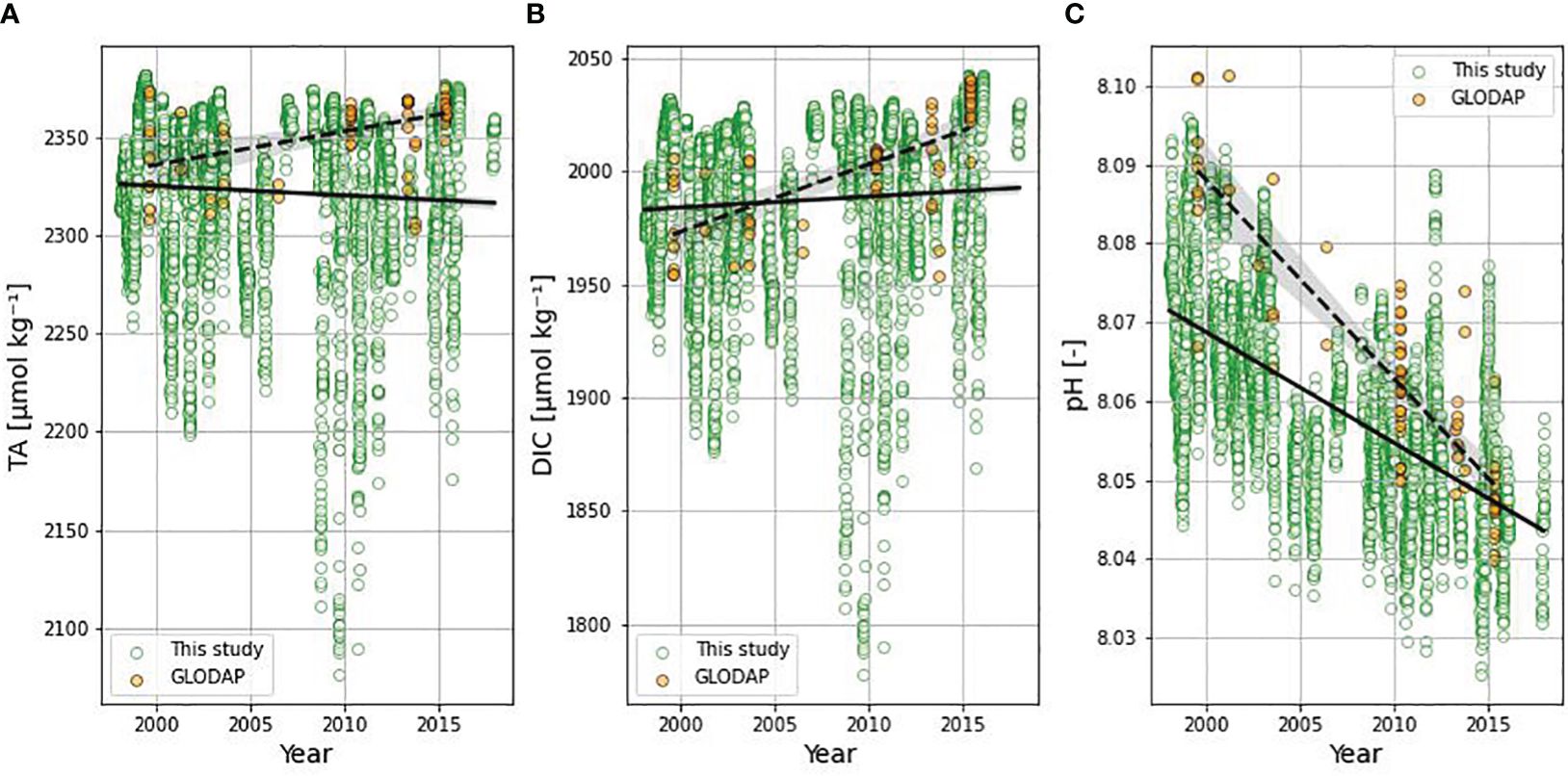
Figure 4 Time series of: (A) TA, (B) DIC, (C) pH. Green dots represent this study’s data and orange dots represents GLODAP’s data from 1998 to 2018, up to 20m depth and between latitudes 3° and 10° N and longitudes of 28° and 42°W. The solid line represents the trend in this study’s data, while the dashed line represents the trend in GLODAP’s data (Lauvset et al., 2022).
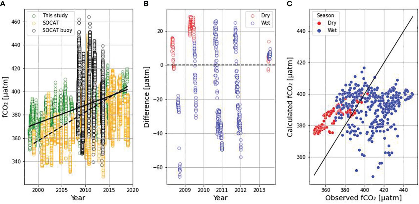
Figure 5 Comparison between fCO2 data calculated in this study and observed fCO2 data from SOCAT (Bakker et al., 2016) from 1998 to 2018 and between latitudes 3° and 10° N and longitudes of 28° and 42° W. (A) Time series with this study’s data (green dots), SOCAT’s data (orange dots) and data from the CARIOCA sensor installed on the buoy from 2008 to 2011 (black dots); (B) Difference between this study’s data and SOCAT’s data (Positive values indicate overestimation and negative values indicate underestimation; red dots represent dry season and blue dots, wet season); (C) Dispersion plot between the two datasets (red and blue dots indicate dry and wet seasons, respectively, and the black line represents the 1: 1 line between the observed data and the calculated data).
3.3 Trends over time
DIC, pH, and fCO2 exhibited significant trends over time based on not de-seasoned data (Table 4). The trends included a yearly increase of 0.7 µmol kg-1 for DIC, a decrease of 0.001 pH units per year for pH, and an increase of 1.539 µatm per year for fCO2 (Figure 6). Notably, when data was de-seasoned, only pH and fCO2 retained significant trends (pH = -0.001 ± 0.000 year-1; fCO2 = +1.633 ± 0.108 µatm year-1) (Figure 7). Additionally, when dry and wet seasons were analyzed separately (Table 5), all variables except SST exhibited significant trends. Notably, the SSS and TA data showed opposing trends between seasons, with positive trends during the dry season and negative trends during the rainy season, emphasizing the seasonal variability. The oceanic xCO2 time series showed and increase around 17% lower than those reported for Barbados station (1.908 ± 0.010 ppm year-1). This delay in our trend related to the atmospheric data highlights the weaker absorption trend of atmospheric CO2 by the WTA.
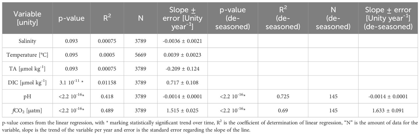
Table 4 Data trend over time for sea surface salinity, temperature, total alkalinity (TA), dissolved inorganic carbon (DIC), pH and CO2 fugacity (fCO2), as well as pH and fCO2 de-seasoned data trends.
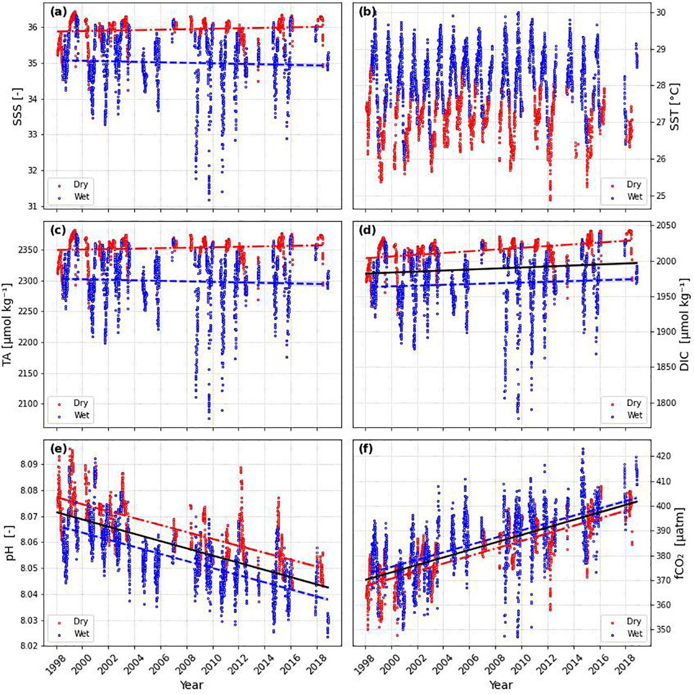
Figure 6 Time series of: (A) Sea Surface Salinity (SSS), (B) Sea Surface Temperature (SST), (C) Total Alkalinity (TA), (D) Dissolved Inorganic Carbon (DIC), (E) pH and (F) Carbon dioxide Fugacity (fCO2). Red dots represent dry season and blue dots represents the wet season. The red dot-dashed line represents the trend in the dry season, the solid black line represents the whole period trend, and the blue dashed line represents the trend in the wet season. Lines are shown only when the trend is statistically significant (p-value< 0.05).
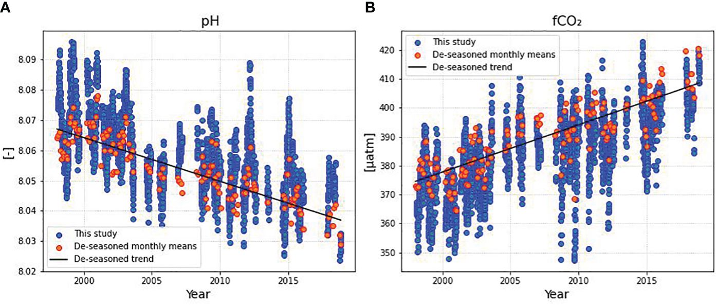
Figure 7 Time series of: (A) pH and (B) fCO2. Blue dots represent the original time series and red dots represents de-seasoned monthly means. Linear trend was calculated based on de-seasoned data.
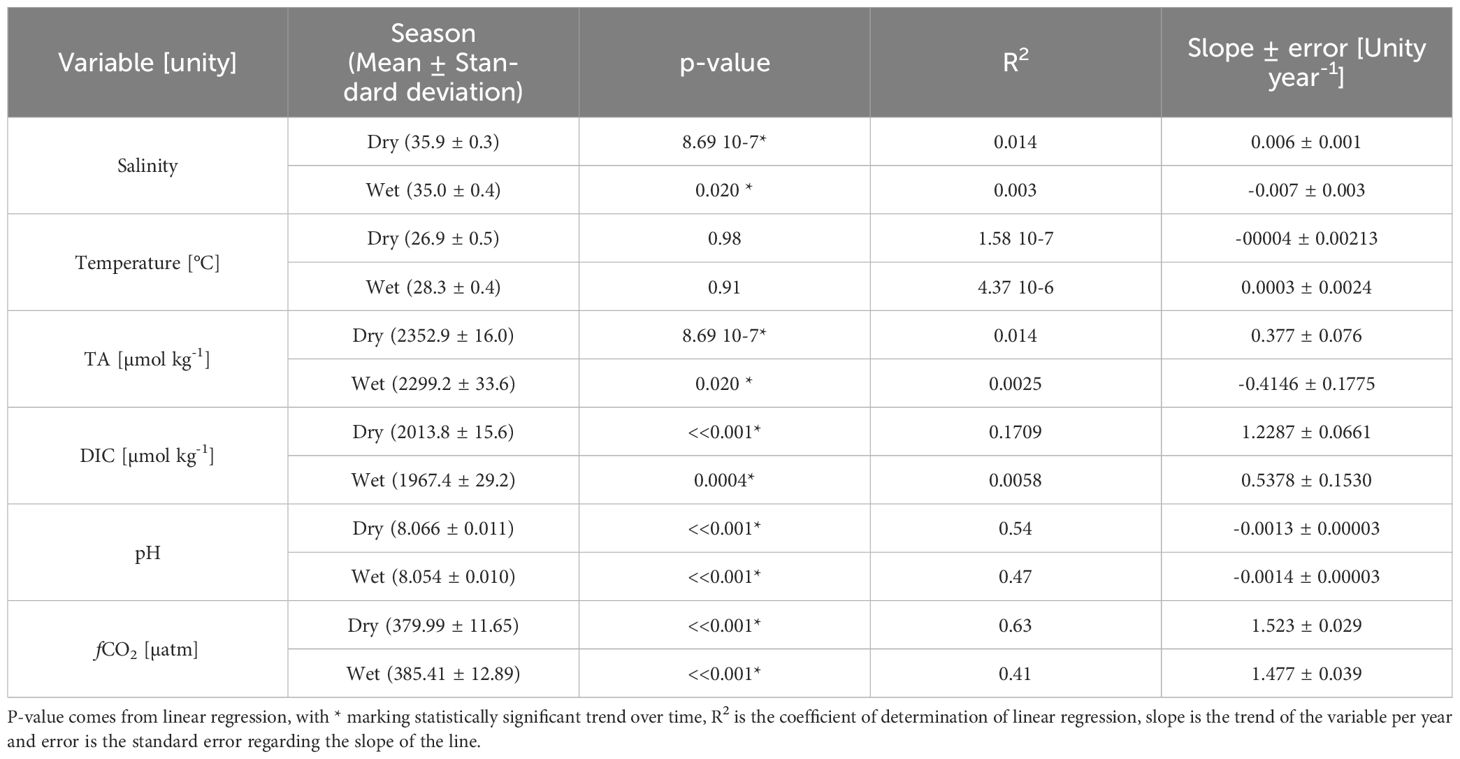
Table 5 Data trend separated in dry (January to June) and wet season (July to December) for sea surface salinity, temperature, total alkalinity (TA), dissolved inorganic carbon (DIC), pH and CO2 fugacity (fCO2).
3.4 Data normalization
The normalization of TA and DIC data (Figure 8) highlighted 3 different aspects of these carbonate parameters: (1) TA-SSS relationship did not vary significantly after normalization, (2) the increase in DIC with time became more apparent (trend of 0.897 ± 0.001 µmol kg-1year-1 and, (3) the normalized pH and fCO2 trends subsequently calculated did not show bigger changes after normalization (-0.001 ± 0.001 and 1.538 ± 0.026, respectively).
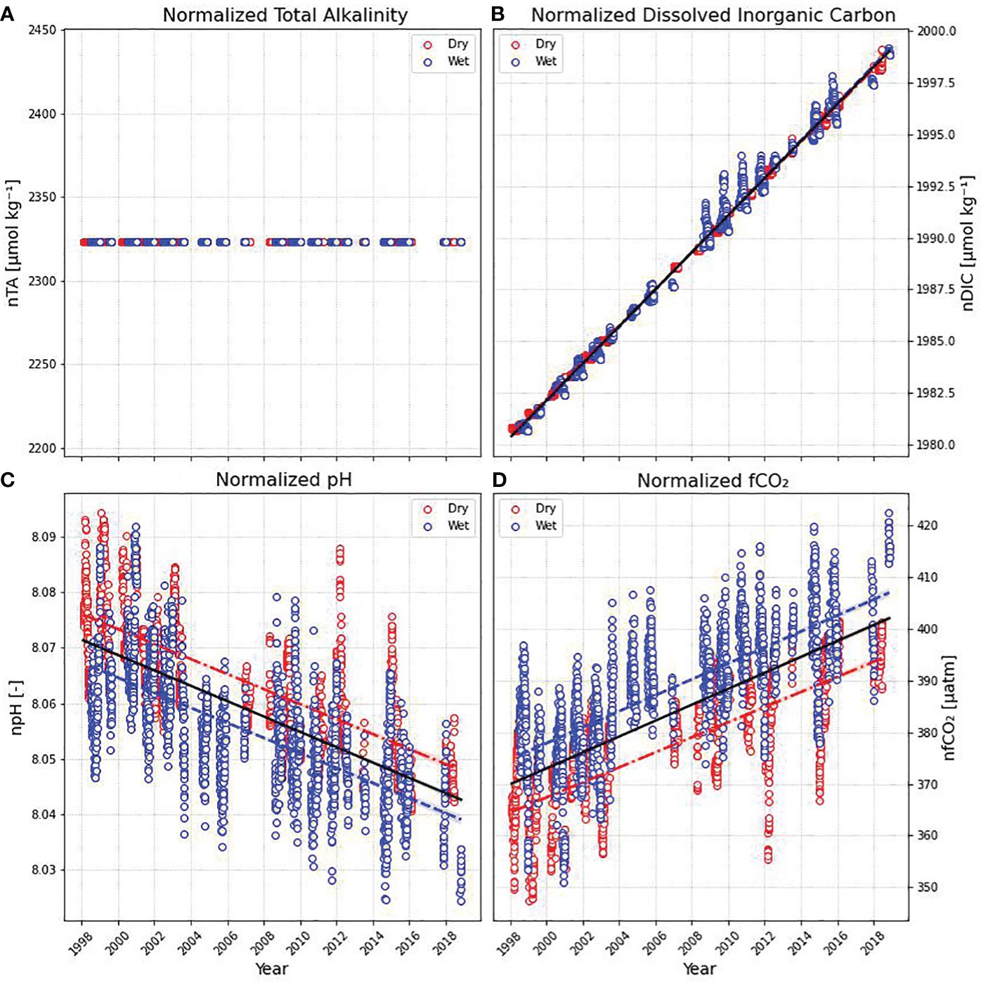
Figure 8 Normalized (A) total alkalinity and (B) dissolved inorganic carbon at mean sea surface salinity of 35.4. Calculated (C) pH and (D) fCO2 based on normalized TA and DIC are also shown. Trend lines are shown for statistically significant trends (red: dry season, blue: wet season and black: all data).
4 Discussion
The study area is susceptible to large seasonal variability in surface salinity (Ffield, 2007; Grodsky et al., 2014) which is reflected in the parameters of the marine carbonate system (Bonou et al., 2016; Bruto et al., 2017). The wet season englobes both the months of the largest discharges of freshwater of the Amazon River and the months in which its waters reach the easternmost area in the Western Tropical Atlantic (Bonou et al., 2016). That and the addition of the rainfall associated to the ITCZ promote a decrease of local sea surface salinity, diluting TA and DIC, as well. These 3 parameters were described by Monteiro et al. (2022) as important drivers of seasonal pCO2 variations in the Western Tropical Atlantic, with DIC and TA being the most expressive one in the NECC region. Thus, it is difficult to capture this variability using available GLODAP in situ data for the region (Lauvset et al., 2022). This emphasizes the importance of using empirical models in the reconstruction of parameters of the marine carbonate system, since these techniques can be used to fill the gaps left by the lack of data in oceanic regions. The lack of in situ data reflecting the temporal and spatial variability in the western tropical Atlantic has also been highlighted by Monteiro et al. (2022). The months from September to November in the years 2008 to 2010 recorded the lowest values of SSS, TA, and DIC (Figure 9). Foltz et al. (2012) attributed this phenomenon to an anomalous sea surface cooling in the Northern Equatorial Atlantic at the beginning of 2009, that caused an abnormal southward shift of the ITCZ over the South American continent. The observed lower salinity is likely associated with the anomalous flood of the Amazon River (Chen et al., 2010).
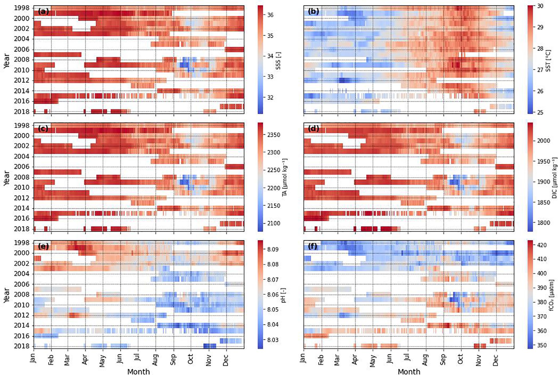
Figure 9 Heatmaps of (A) SSS, (B) SST, (C) TA, (D) DIC, (E) pH and (F) fCO2. Each cell represents a daily value.
Based on the analysis done in this study, the calculated fCO2 data exhibited a slight upward deviation when compared to the corresponding data from the SOCAT database (Figure 5A). However, this difference was relatively small, with a median ratio of 0.45%. Interestingly, upon excluding data from the buoy, this disparity noticeably increased to 2.88%. It is noteworthy that the buoy dataset, characterized by a higher frequency and greater variability, played a significant role in mitigating the observed deviation. During the period with buoy data, though, SOCAT data exhibited a higher amplitude that our calculations did not fully capture. Daily averages of the data measured by the sensor installed in the buoy showed that our calculations mostly overestimated the fCO2 values, particularly during the dry season (Figure 5B), where an overestimation of 3.11% was found when comparing the medians. This might be a result of the models used to calculate the TA and DIC that are based on the whole Western Tropical Atlantic area, which includes areas with higher salinity and lower influences of the Amazon River plume and ITCZ (Araujo et al., 2019; Bonou et al., 2022). The difference is more variable during the wet season, but still our calculations tend to underestimate the fCO2 in the area by roughly 5.51%. Considering the biological impacts in ocean carbonate parameters in the models used in this study might also affect the calculations, especially in the wet season, a time when the high nutrient plume reaches eastern parts of the Tropical Atlantic. The enhancement of primary production in the Western Tropical Atlantic by the nutrient rich Amazon River Plume is estimated to increase the oceanic’s capacity of absorbing atmospheric CO2 from 30% to even 100 times (Ternon et al., 2000; Cooley et al., 2007). It is possible to see that there is no 1:1 ratio (Figure 5C) between the data calculated in this study and the data from the sensor. However, when comparing with the graph made by Bonou et al. (2016) it is observed that, for data from the NECC region, the distribution of points of the data used in this study is similar to the point cloud showed by the aforementioned authors. This variation may be a result of primary productivity being enhanced at the region once the Amazon River plume brings waters richer in nutrients when compared to the surrounding ocean (Lefèvre et al., 2017).
The SSS, SST and fCO2 values in dry and wet seasons are in accordance to those found by Lefèvre et al. (2014) in March 2009 and July 2010 during the PIRATA XI and XII commissions, respectively. In March 2009 (July 2010), they observed an average SSS of 35.89 ± 0.17 (35.75 ± 0.6), an average SST of 26.3 ± 0.8°C (28.67 ± 0.72°C) and average fCO2 of 374.3 ± 13 µatm (381.2 ± 11.8 µatm). The authors discuss the possible drivers of fCO2 variability in the region, bringing the influence of the ITCZ as an important factor in that regard. The highest values of fCO2 happening during wet season coincides with the upwelling period observed by Bruto et al. (2017) in the same study region. The authors calculated Ekman pumping from monthly wind averages with a spatial scale of 0.25° and identified that upwelling is more intense in the second half of the year, injecting CO2-rich subsurface waters into the surface.
Bonou et al. (2016) found similar values to those presented in this study for SSS, SST, TA and DIC, also separating into two seasons. The average values of the dry season (SSS = 35.4 ± 0.7, SST = 27.6 ± 1.1°C, TA = 2331 ± 54 µmol kg-1, DIC = 1978 ± 45 µmol kg-1), and of the wet season (SSS = 35.2 ± 0.8, SST = 28.1 ± 0.8°C, TA = 2328 ± 48 µmol kg- 1, DIC = 1970 ± 42 µmol kg-1) also show accuracy of these models in estimating the TA and DIC in the region. The models also showed values close to the GLODAP TA, DIC and pH data (Figure 4), with the database values in the range of the calculated parameters. When compared to the results of Bonou et al. (2022) in the Western Atlantic, we can see the mean values of TA and DIC values calculated here are higher than the ones found by them. These differences show once more the heterogeneity of the region, especially when the Amazon River Plume region (western to 43°W) is added to the equation.
The combination of the intense rainfall (Figure 3A) and the Amazon River plume (Richey et al., 1989; Silva et al., 2010; Marengo and Espinoza, 2016), leads to lower surface salinity during the wet season. This, along with heating and reduced vertical mixing due to surface water stratification from added fresh water, explains higher temperatures in stronger upwelling seasons. This can also lead to the formation of more severe storms and hurricanes of higher categories (Ffield, 2007; Grodsky et al., 2012). The upwelling of subsurface water generated by tropical storm winds plays an important role in high frequency variations (less than one day) in fCO2, thus affecting the CO2 flux in the region (Mahadevan et al., 2011; Bruto et al., 2017).
Studies investigating the trend in carbonate parameters in the Atlantic Ocean show the heterogeneity of the area and how the Western Tropical Atlantic might fit in the dynamics of the region. Lauvset et al. (2015) observed for the Equatorial Atlantic biome (between 5° S and 5° N) a pH trend of -0.0016 ± 0.0003 units year-1 and fCO2 trend of 1.81 ± 0.32 µatm year-1, which is in accordance to the trends observed in this study.
Further north, in the Cariaco basin, Venezuela, the CARIACO time series (CArbon Retention In A Colored Ocean, 10.5°N- 64.67°W) was conducted, with TA and pH measurements taken from 1995 to 2015 (Table 6). Bates et al. (2014) observed a significant trend in pH (-0.0025 ± 0.0004 year-1) which was greater than the trend observed in this study. Due to its location further west in the Caribbean Sea compared to the PIRATA buoy at 8°N, other factors such as regional circulation or its position over a trench may influence the local carbonate system differently than in oceanic areas (Astor et al., 2017, 2013, 2005; Muller-Karger et al., 2001).
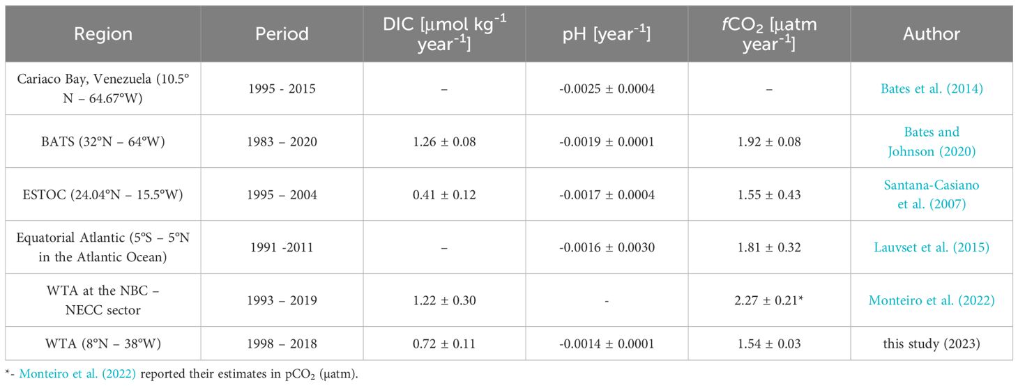
Table 6 Trends in the surface carbonate system in the western Tropical Atlantic Ocean used for comparison in this study.
At the BATS time series station (Bermuda Atlantic Time-series Study, 32°N, 64°W), in operation since 1983, Bates and Johnson (2020) calculated the time trends of marine carbonate system parameters up to 2020. The DIC time trend values (1.26 ± 0.04 μmol kg-1 year-1), pH (-0.0019 ± 0.0001 pH units year-1), and fCO2 (1.92 ± 0.08 μatm year-1) were higher in magnitude than those found in this study. Unlike the BATS station, the western Tropical Atlantic does not exhibit the trend of seawater salinization, but rather shows a desalinization trend during the wet season. This indicates a possible intensification of the hydrological cycle, which could impact the CO2 dynamics in the area in the future (Byrne et al., 2018).
At the Eastern Tropical Atlantic Ocean, the European Station for Time series in the Ocean at the Canary Islands (ESTOC, 29.04°N-15.5°W), maintains a monitoring base similar to BATS, where measurements started in 1995. Santana-Casiano et al. (2007) observed an increasing trend in the DIC (0.41 ± 0.12 µmol kg-1 year-1) smaller than the one found in this study, a trend towards a reduction in pH (-0.0017 ± 0.0004 pH units year-1) and tendency of increase in fCO2 (1.55 ± 0.43 µatm year-1) close to those observed in this study. Although this station is in the eastern Atlantic Ocean, a region with a very marked and almost permanent upwelling, its annual trends are closer to the trends found in this study than those found in BATS, which is also on the western edge.
According to Monteiro et al. (2022), SSS only acts as the main driver in pCO2 variations in the Amazon River Plume region (being responsible for the biggest variation in the regional values), with the SST being the main driver of pCO2 variations in NECC region. This is contradicted by our results, since after calculating the thermal to non-thermal effects ratio on fCO2 described by Takahashi et al. (2002) we arrived at a value of 0.82, indicating that biological effects override thermal effects in CO2 variations in our area. It is important to note that the high SSS variation closer to the river might impact the results of the calculations (Jiang et al., 2014). In addition, Monteiro et al. (2022) found a trend around 2.27 ± 0.21 µatm year-1, roughly 50% higher than the trend we found in this study. However, the temperature normalized pCO2 presented a trend in time closer to the one observed in this study (1.56 ± 0.26 µatm year-1), indicating that the pCO2 estimations in the NECC using the models utilized in this study tend to leave out the impact of changes in temperature (Takahashi et al., 2002).
The SST did not show a significant trend in this study, unlike neighboring regions such as the central tropical Atlantic and the Sargasso Sea, in the subtropical Atlantic, which showed an increase of 0.009 and 0.021°C year-1, respectively (Deser et al., 2010; Bates and Johnson, 2020). In agreement with the data showed in this study, Friedman et al. (2017) observed that the area in this study showed no statistically significant SSS trend from 1896 to 2013 (118 years), although some studies indicate that there is a tendency towards salinization in the tropical and subtropical Atlantic Ocean (Boyer, 2005; Bates and Johnson, 2020). SSS showed, nonetheless, a trend in time only after separating data in two seasons, which might indicate a change in the hydrological cycle in the area, possibly leading to changes in the CO2 solubility in the region (Ashton et al., 2016).
In oceanic areas, trends in pH and fCO2 mainly respond to DIC fluxes on the surface, reflecting the increase in the concentration of atmospheric CO2 (Lauvset et al., 2015). In the NECC region, in addition to DIC, temperature is an important driver in fCO2 (Monteiro et al., 2022), since the physical pump is the main driver of CO2 drawdown. Taking that in account, the lack of a temperature factor in the models for TA and DIC in the NECC area might underestimate the results for a region with less impact from the Amazon River Plume but still susceptible to high salinity seasonality.
The DIC/TA ratio is a key indicator of the acid-base equilibrium in seawater (Cai et al., 2020). A trend of 0.0004 ± 5.7 10-7 year-1 is observed in the study area (Figure 10A), indicating a decrease in its buffer capacity. In addition, the difference between total alkalinity and dissolved inorganic carbon (TA-DIC) is also a good tool to imply the ocean acidification (Figure 10B), with the advantage of being a conservative quantity, particularly useful in studies involving the mixing of different water masses. In this study, the TA-DIC showed a decrease of 0.93 ± 0.02 µmol kg-1 year-1, reinforcing again the decrease in buffer capacity of the region. Xue and Cai (2020) estimated a decrease in TA-DIC of around 0.82 µmol kg-1 year-1 at Hawaii Ocean Time-series (HOT) station. Their results suggest that the Western Tropical Atlantic is absorbing atmospheric CO2 at a more pronounced rate.
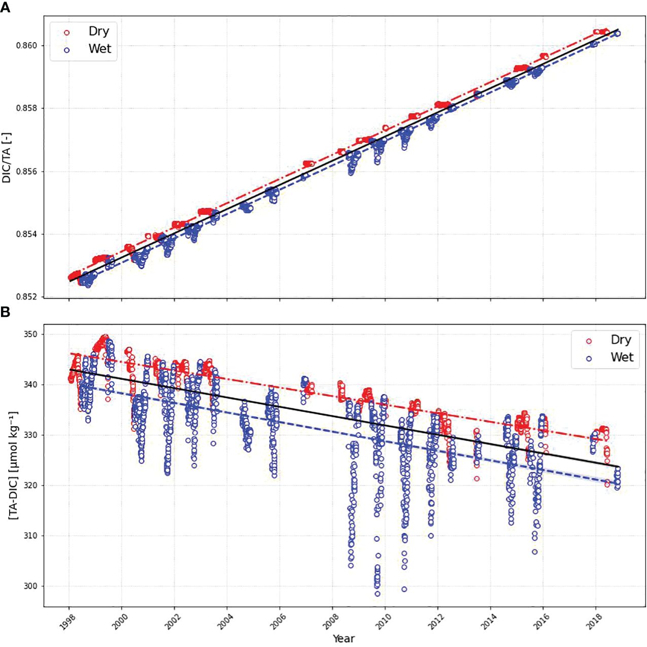
Figure 10 Time series of: (A) DIC/TA and (B) [TA-DIC]. Red dots represent dry season and blue dots represents the wet season. The red dot-dashed line represents the trend in the dry season, the solid black line represents the whole period trend, and the blue dashed line represents the trend in the wet season. Lines are shown only when the trend is statistically significant (p-value< 0.05).
5 Conclusion
Showcasing a temporal overview of the marine carbonate system at 8°N 38°W between 1998 and 2018, our study focuses on a region distinguished by pronounced salinity variations compared to other tropical oceanic areas. This study highlights the seasonality of Total Alkalinity (TA), Dissolved Inorganic Carbon (DIC), pH, and fCO2 in the Western Tropical Atlantic (WTA), a phenomenon previously observed only on a limited time scale (Bruto et al., 2017) or across extensive spatial dimensions with intermittent temporal continuity (Körtzinger, 2003; Lefévre et al., 2010; Bonou et al., 2016). In this study, no significant SSS trend was observed from 1998 to 2018, agreeing with the trend calculated from data collected in situ in the Atlantic in the same region from 1896 to 2013 (Friedman et al., 2017), although a positive and negative trend can be observed in dry and wet seasons, respectively. This could possibly lead to the increase of high frequency variability in fCO2 due to upwelling by tropical storm winds (Ffield, 2007; Mahadevan et al., 2011; Grodsky et al., 2012). SST also showed no significant trend, diverging from studies showing an increase in SST both in the Central Tropical Atlantic and in the BATS time series (Deser et al., 2010; Bates and Johnson, 2020).
From the comparison with other studies analyzing the trend of parameters in the marine carbonate system in the tropical and subtropical Atlantic, it was observed that the increase in DIC and fCO2, in addition to the reduction in pH, were smaller when compared to the observed trends in CARIACO and BATS (Bates et al., 2014; Bates and Johnson, 2020). On the other hand, the ESTOC station, on the eastern edge of the Tropical Atlantic, showed a smaller increase in DIC, a stronger reduction in pH and an increase in fCO2 similar to the trends found in this study. Finally, when evaluating the pH variation and CO2 fugacity in the Equatorial Atlantic biome (5°S to 5°N) from 1911 to 2011, it was observed that the reduction in pH and increase in fCO2 were close to the trends observed in this study (Lauvset et al., 2015).
In conclusion, the use of empirical models as proposed in this study is an approach that can be successfully used for filling the gap regarding the marine carbonate system in the Western Tropical Atlantic, a region with marked data scarcity.
Data availability statement
The original contributions presented in the study are included in the article/Supplementary Material. Further inquiries can be directed to the corresponding author.
Author contributions
CM: Conceptualization, Data curation, Formal analysis, Investigation, Methodology, Writing – original draft, Writing – review & editing. LC: Conceptualization, Formal analysis, Investigation, Methodology, Supervision, Writing – review & editing. LP: Supervision, Writing – review & editing. AF: Writing – review & editing. MA: Writing – review & editing.
Acknowledgments
The author(s) declare financial support was received for the research, authorship, and/or publication of this article. We are grateful for the PIRATA program for the installation and maintenance of the mooring site, as well as the availability of online data on salinity, temperature, precipitation and fCO2. We would also like to thank GLODAP for the online availability of TA, DIC and pH data for the region. In addition, we are also thankful for the SOCAT platform for providing the buoy fCO2 data. LC (CNPq grant 309708/2021–4, FAPERJ grant E-26/201.156/2022, Prociência/UERJ grant) and MA thank the support of the Brazilian Research Network on Global Climate Change - Rede CLIMA (FINEP-CNPq 437167/2016–0), and the Amazon Coastal Observatory (OCA). We are grateful to Ocean Data View for making freely available the software where the study area maps for this study were made. This study was funded in part by the Coordenação de Aperfeiçoamento de Pessoal de Nível Superior - Brasil (CAPES) - Finance Code 001. CM acknowledges CAPES M.Sc. grant no. 88882.450349/2019–01. This is a contribution to the International Joint Laboratory TAPIOCA (IRD and CAPES/MEC), to the TRIATLAS project, which has received funding from the European Union’s Horizon 2020 research and innovation program under grant agreement No 817578, and to the Brazilian Ocean Acidification Research Network – BrOA.
Conflict of interest
The authors declare that the research was conducted in the absence of any commercial or financial relationships that could be construed as a potential conflict of interest.
Publisher’s note
All claims expressed in this article are solely those of the authors and do not necessarily represent those of their affiliated organizations, or those of the publisher, the editors and the reviewers. Any product that may be evaluated in this article, or claim that may be made by its manufacturer, is not guaranteed or endorsed by the publisher.
Supplementary material
The Supplementary Material for this article can be found online at: https://www.frontiersin.org/articles/10.3389/fmars.2024.1286960/full#supplementary-material
Supplementary Material 1 | Time series of: (A) Sea Surface Salinity (SSS) and (B) Sea Surface Temperature (SST). Blue dots represent all data available for the period at the buoy and red triangles represent the daily means of the data.
References
A’Hearn P. N., Freitag H. P., McPhaden M. J. (2002). ATLAS module temperature bias due to solar heating Vol. 28 Springfield, VA. (NOAA Technical Memorandum OAR PMEL-1). Available at: https://permanent.fdlp.gov/websites/www.pmel.noaa.gov/pdf-archive/ahea2486.pdf.
Allen R., Foggo A., Fabricius K., Balistreri A., Hall-Spencer J. M. (2017). Tropical CO2 seeps reveal the impact of ocean acidification on coral reef invertebrate recruitment. Mar. Pollut. Bull. 124, 607–613. doi: 10.1016/j.marpolbul.2016.12.031
Allen M. R., Frame D. J., Huntingford C., Jones C. D., Lowe J. A., Meinshausen M., et al. (2009). Warming caused by cumulative carbon emissions towards the trillionth tonne. Nature 458, 1163–1166. doi: 10.1038/nature08019
Araujo M., Noriega C., Hounsou-gbo G. A., Veleda D., Araujo J., Bruto L., et al. (2017). A synoptic assessment of the amazon river-ocean continuum during boreal autumn: from physics to plankton communities and carbon flux. Front. Microbiol. 8. doi: 10.3389/fmicb.2017.01358
Araujo M., Noriega C., Medeiros C., Lefèvre N., Ibánhez J. S. P., Flores M., et al. (2019). On the variability in the CO 2 system and water productivity in the western tropical Atlantic off North and Northeast Brazil. J. Mar. Syst. 189, 62–77. doi: 10.1016/j.jmarsys.2018.09.008
Ashton I. G., Shutler J. D., Land P. E., Woolf D. K., Quartly G. D. (2016). A sensitivity analysis of the impact of rain on regional and global sea-air fluxes of CO2. PloS One 11, e0161105. doi: 10.1371/journal.pone.0161105
Astor Y. M., Lorenzoni L., Guzman L., Fuentes G., Muller-Karger F., Varela R., et al. (2017). Distribution and variability of the dissolved inorganic carbon system in the Cariaco Basin, Venezuela. Mar. Chem. 195, 15–26. doi: 10.1016/j.marchem.2017.08.004
Astor Y. M., Lorenzoni L., Thunell R., Varela R., Muller-Karger F., Troccoli L., et al. (2013). Interannual variability in sea surface temperature and fCO2 changes in the Cariaco Basin. Deep Sea Res. Part II: Topical Stud. Oceanogr. 93, 33–43. doi: 10.1016/j.dsr2.2013.01.002
Astor Y. M., Scranton M. I., Muller-Karger F., Bohrer R., García J. (2005). fCO2 variability at the CARIACO tropical coastal upwelling time series station. Mar. Chem. 97, 245–261. doi: 10.1016/j.marchem.2005.04.001
Baker H. S., Millar R. J., Karoly D. J., Beyerle U., Guillod B. P., Mitchell D., et al. (2018). Higher CO2 concentrations increase extreme event risk in a 1.5°c world. Nat. Climate Change 8, 604–608. doi: 10.1038/s41558-018-0190-1
Bakker D. C. E., Pfeil B., Landa C. S., Metzl N., O’Brien K. M., Olsen A., et al. (2016). A multi-decade record of high-quality fCO2 data in version 3 of the Surface Ocean CO2 Atlas (SOCAT). Earth System Sci. Data 8, 383–413. doi: 10.5194/essd-8-383-2016
Bates N. R., Astor Y. M., Church M. J., Currie K., Dore J. E., González-Dávila M., et al. (2014). A time-series view of changing surface ocean chemistry due to ocean uptake of anthropogenic CO2 and ocean acidification. Oceanography 27, 126–141. doi: 10.5670/oceanog.2014.16
Bates N. R., Johnson R. J. (2020). Acceleration of ocean warming, salinification, deoxygenation and acidification in the surface subtropical North Atlantic Ocean. Commun. Earth Environ. 1, 33. doi: 10.1038/s43247-020-00030-5
Bednaršek N., Feely R. A., Howes E. L., Hunt B. P. V., Kessouri F., León P., et al. (2019). Systematic review and meta-analysis toward synthesis of thresholds of ocean acidification impacts on calcifying pteropods and interactions with warming. Front. Mar. Sci. 6. doi: 10.3389/fmars.2019.00227
Bignami S., Sponaugle S., Cowen R. K. (2013). Response to ocean acidification in larvae of a large tropical marine fish, Rachycentron canadum. Global Change Biol. 19, 996–1006. doi: 10.1111/gcb.12133
Bonou F., Medeiros C., Noriega C., Araujo M., Hounsou-Gbo A., Lefèvre N. (2022). A comparative study of total alkalinity and total inorganic carbon near tropical Atlantic coastal regions. J. Coast. Conserv. 26, 31. doi: 10.1007/s11852-022-00872-5
Bonou F. K., Noriega C., Lefèvre N., Araujo M. (2016). Distribution of CO2 parameters in the western tropical atlantic ocean. Dynamics Atmospheres Oceans 73, 47–60. doi: 10.1016/j.dynatmoce.2015.12.001
Bourlès B., Araujo M., McPhaden M. J., Brandt P., Foltz G. R., Lumpkin R., et al. (2019). PIRATA: A sustained observing system for tropical atlantic climate research and forecasting. Earth Space Sci. 6, 577–616. doi: 10.1029/2018EA000428
Boyer T. P. (2005). Linear trends in salinity for the World Ocean 1955–1998. Geophysical Res. Lett. 32, L01604. doi: 10.1029/2004GL021791
Bruto L., Araujo M., Noriega C., Veleda D., Lefèvre N. (2017). Variability of CO2 fugacity at the western edge of the tropical Atlantic Ocean from the 8°N to 38°W PIRATA buoy. Dynamics Atmospheres Oceans 78, 1–13. doi: 10.1016/j.dynatmoce.2017.01.003
Buapet P., Gullström M., Björk M. (2013). Photosynthetic activity of seagrasses and macroalgae in temperate shallow waters can alter seawater pH and total inorganic carbon content at the scale of a coastal embayment. Mar. Freshw. Res. 64, 1040–1048. doi: 10.1071/MF12124
Byrne M. P., Pendergrass A. G., Rapp A. D., Wodzicki K. R. (2018). Response of the intertropical convergence zone to climate change: location, width, and strength. Curr. Clim Change Rep. 4, 355–370. doi: 10.1007/s40641-018-0110-5
Cai W.-J., Xu Y.-Y., Feely R. A., Wanninkhof R., Jönsson B., Alin S. R., et al. (2020). Controls on surface water carbonate chemistry along North American ocean margins. Nat. Commun. 11, 2691. doi: 10.1038/s41467-020-16530-z
Chen J. L., Wilson C. R., Tapley B. D. (2010). The 2009 exceptional Amazon flood and interannual terrestrial water storage change observed by GRACE. Water Resour. Res. 46. doi: 10.1029/2010WR009383
Cooley S. R., Coles V. J., Subramaniam A., Yager P. L. (2007). Seasonal variations in the Amazon plume-related atmospheric carbon sink. Global Biogeochem. Cycles 21, GB3014. doi: 10.1029/2006GB002831
De Boyer Montégut C., Madec G., Fischer A. S., Lazar A., Iudicone D. (2004). Mixed layer depth over the global ocean: An examination of profile data and a profile-based climatology. J. Geophys. Res. 109, 2004JC002378. doi: 10.1029/2004JC002378
de Carvalho-Borges M., Orselli I. B. M., de Carvalho Ferreira M. L., Kerr R. (2018). Seawater acidification and anthropogenic carbon distribution on the continental shelf and slope of the western South Atlantic Ocean. J. Mar. Syst. 187, 62–81. doi: 10.1016/j.jmarsys.2018.06.008
Deser C., Phillips A. S., Alexander M. A. (2010). Twentieth century tropical sea surface temperature trends revisited. Geophysical Res. Lett. 37, L10701. doi: 10.1029/2010GL043321
Dickson A. G. (1981). An exact definition of total alkalinity and a procedure for the estimation of alkalinity and total inorganic carbon from titration data. Deep-Sea Res. Part a-Oceanographic Res. Pap. 28, 609–623. doi: 10.1016/0198-0149(81)90121-7
Dickson A. G. (1990). Standard potential of the reaction: AgCl(s) + 1 2H2(g) = Ag(s) + HCl(aq), and and the standard acidity constant of the ion HSO4- in synthetic sea water from 273.15 to 318.15 K. J. Chem. Thermodynamics 22, 113–127. doi: 10.1016/0021-9614(90)90074-Z
Dickson A. G., Sabine C. L., Christian J. R. (eds) (2007). Guide to Best Practices for Ocean CO2 measurements. PICES Special Publication, Guide to Best Practices for Ocean CO2 measurements (PICES Special Publication). doi: 10.25607/OBP-1342
Doney S. C., Fabry V. J., Feely R. A., Kleypas J. A. (2009). Ocean acidification: the other CO 2 problem. Annu. Rev. Mar. Sci. 1, 169–192. doi: 10.1146/annurev.marine.010908.163834
Dugdale R. C., Wischmeyer A. G., Wilkerson F. P., Barber R. T., Chai F., Jiang M.-S., et al. (2002). Meridional asymmetry of source nutrients to the equatorial Pacific upwelling ecosystem and its potential impact on ocean–atmosphere CO2 flux; a data and modeling approach. Deep Sea Res. Part II: Topical Stud. Oceanogr. 49, 2513–2531. doi: 10.1016/S0967-0645(02)00046-2
Emerson S., Hedges J. (2008). Chemical Oceanography and the Marine Carbon cycle (Cambridge: Cambridge University Press). doi: 10.1017/CBO9780511793202
Fassbender A. J., Alin S. R., Feely R. A., Sutton A. J., Newton J. A., Byrne R. H. (2017). Estimating total alkalinity in the washington state coastal zone: complexities and surprising utility for ocean acidification research. Estuaries Coasts 40, 404–418. doi: 10.1007/s12237-016-0168-z
Ffield A. (2007). Amazon and orinoco river plumes and NBC rings: bystanders or participants in hurricane events? J. Climate 20, 316–333. doi: 10.1175/JCLI3985.1
Foltz G. R., Brandt P., Richter I., Rodríguez-Fonseca B., Hernandez F., Dengler M., et al. (2019). The tropical atlantic observing system. Front. Mar. Sci. 6. doi: 10.3389/fmars.2019.00206
Foltz G. R., McPhaden M. J., Lumpkin R. (2012). A strong atlantic meridional mode event in 2009: the role of mixed layer dynamics*. J. Climate 25, 363–380. doi: 10.1175/JCLI-D-11-00150.1
Freitag H. P., Mccarty M. E., Nosse C., Lukas R., Mcphaden M. J., Cronin M. F., et al. (1999). COARE Seacat data: Calibrations and quality control procedures (Springfield, VA: NOAA Technical Memorandum ERL PMEL-1), 1–93.
Freitag H. P., Sawatzky T. A., Ronnholm K. B., J. M. M. (2005). Calibration procedures and instrumental accuracy estimates of next generation ATLAS water temperature and pressure measurements (Springfield, VA: NOAA Technical Memorandum OAR PMEL-1).
Friedlingstein P., Jones M. W., O’Sullivan M., Andrew R. M., Bakker D. C. E., Hauck J., et al. (2022). Global carbon budget 2021. Earth Syst. Sci. Data 14, 1917–2005. doi: 10.5194/essd-14-1917-2022
Friedman A. R., Reverdin G., Khodri M., Gastineau G. (2017). A new record of Atlantic sea surface salinity from 1896 to 2013 reveals the signatures of climate variability and long-term trends. Geophysical Res. Lett. 44, 1866–1876. doi: 10.1002/2017GL072582
Friis K., Körtzinger A., Wallace D. W. R. (2003). The salinity normalization of marine inorganic carbon chemistry data. Geophysical Res. Lett. 30, 2002GL015898. doi: 10.1029/2002GL015898
Goodwin P., Lenton T. M. (2009). Quantifying the feedback between ocean heating and CO 2 solubility as an equivalent carbon emission. Geophysical Res. Lett. 36, L15609. doi: 10.1029/2009GL039247
Gouretski V. V., Koltermann K. P. (2004). WOCE Global Hydrographic Climatology A Technical Report (No. 35/2004) (Bundesamtes für Seeschifffahrt und Hydrographie).
Grodsky S. A., Reul N., Lagerloef G., Reverdin G., Carton J. A., Chapron B., et al. (2012). Haline hurricane wake in the Amazon/Orinoco plume: AQUARIUS/SACD and SMOS observations. Geophysical Res. Lett. 39, 2012GL053335. doi: 10.1029/2012GL053335
Grodsky S. A., Reverdin G., Carton J. A., Coles V. J. (2014). Year-to-year salinity changes in the Amazon plume: Contrasting 2011 and 2012 Aquarius/SACD and SMOS satellite data. Remote Sens. Environ. 140, 14–22. doi: 10.1016/j.rse.2013.08.033
Guinotte J. M., Fabry V. J. (2008). Ocean acidification and its potential effects on marine ecosystems. Ann. New York Acad. Sci. 1134, 320–342. doi: 10.1196/annals.1439.013
Humphreys M. P., Lewis E. R., Sharp J. D., Pierrot D. (2022). PyCO2SYS v1.8: marine carbonate system calculations in Python. Geosci. Model. Dev. 15, 15–43. doi: 10.5194/gmd-15-15-2022
Jiang Z.-P., Tyrrell T., Hydes D. J., Dai M., Hartman S. E. (2014). Variability of alkalinity and the alkalinity-salinity relationship in the tropical and subtropical surface ocean. Global Biogeochemical Cycles 28, 729–742. doi: 10.1002/2013GB004678
Körtzinger A. (2003). A significant CO2 sink in the tropical Atlantic Ocean associated with the Amazon River plume. Geophysical Res. Lett. 30, 2–5. doi: 10.1029/2003GL018841
Kroeker K. J., Kordas R. L., Crim R. N., Singh G. G. (2010). Meta-analysis reveals negative yet variable effects of ocean acidification on marine organisms. Ecol. Lett. 13, 1419–1434. doi: 10.1111/j.1461-0248.2010.01518.x
Lauvset S. K., Gruber N., Landschützer P., Olsen A., Tjiputra J. (2015). Trends and drivers in global surface ocean pH over the past 3 decades. Biogeosciences 12, 1285–1298. doi: 10.5194/bg-12-1285-2015
Lauvset S. K., Lange N., Tanhua T., Bittig H. C., Olsen A., Kozyr A., et al. (2022). GLODAPv2.2022: the latest version of the global interior ocean biogeochemical data product. Earth Syst. Sci. Data 14, 5543–5572. doi: 10.5194/essd-14-5543-2022
Lee K., Tong L. T., Millero F. J., Sabine C. L., Dickson A. G., Goyet C., et al. (2006). Global relationships of total alkalinity with salinity and temperature in surface waters of the world’s oceans. Geophysical Res. Lett. 33, 1–5. doi: 10.1029/2006GL027207
Lefévre N., Diverrés D., Gallois F. (2010). Origin of CO 2 undersaturation in the western tropical Atlantic. Tellus B: Chem. Phys. Meteorol. 62, 595–607. doi: 10.1111/j.1600–0889.2010.00475.x
Lefèvre N., Guillot A., Beaumont L., Danguy T. (2008). Variability of fCO2in the Eastern Tropical Atlantic from a moored buoy. J. Geophysical Res.: Oceans 113, 1–12. doi: 10.1029/2007JC004146
Lefèvre N., Montes M. F., Gaspar F. L., Rocha C., Jiang S., De Araújo M. C., et al. (2017). Net heterotrophy in the Amazon continental shelf changes rapidly to a sink of CO2 in the outer Amazon plume. Front. Mar. Sci. 4. doi: 10.3389/fmars.2017.00278
Lefèvre N., Urbano D. F., Gallois F., Diverrès D. (2014). Impact of physical processes on the seasonal distribution of the fugacity of CO 2 in the western tropical Atlantic. J. Geophysical Res.: Oceans 119, 646–663. doi: 10.1002/2013JC009248
Mahadevan A., Tagliabue A., Bopp L., Lenton A., Mémery L., Lévy M. (2011). Impact of episodic vertical fluxes on sea surface pCO 2. Philos. Trans. R. Soc. A: Mathematical Phys. Eng. Sci. 369, 2009–2025. doi: 10.1098/rsta.2010.0340
Mangi S. C., Lee J., Pinnegar J. K., Law R. J., Tyllianakis E., Birchenough S. N. R. (2018). The economic impacts of ocean acidification on shellfish fisheries and aquaculture in the United Kingdom. Environ. Sci. Policy 86, 95–105. doi: 10.1016/j.envsci.2018.05.008
Mardani A., Streimikiene D., Cavallaro F., Loganathan N., Khoshnoudi M. (2019). Carbon dioxide (CO2) emissions and economic growth: A systematic review of two decades of research from 1995 to 2017. Sci. Total Environ. 649, 31–49. doi: 10.1016/j.scitotenv.2018.08.229
Marengo J. A., Espinoza J. C. (2016). Extreme seasonal droughts and floods in Amazonia: causes, trends and impacts. Int. J. Climatol. 36, 1033–1050. doi: 10.1002/joc.4420
Marion G. M., Millero F. J., Camões M. F., Spitzer P., Feistel R., Chen C. T. A. (2011). PH of seawater. Mar. Chem. 126, 89–96. doi: 10.1016/j.marchem.2011.04.002
McGillis W. R., Edson J. B., Zappa C. J., Ware J. D., McKenna S. P., Terray E. A., et al. (2004). Air-sea CO 2 exchange in the equatorial Pacific. J. Geophysical Res.: Oceans 109, C08S02. doi: 10.1029/2003JC002256
Merlivat L., Boutin J., Antoine D. (2015). Roles of biological and physical processes in driving seasonal air-sea CO2 flux in the Southern Ocean: New insights from CARIOCA pCO2. J. Mar. Syst. 147, 9–20. doi: 10.1016/j.jmarsys.2014.04.015
Middelburg J. J., Soetaert K., Hagens M. (2020). Ocean alkalinity, buffering and biogeochemical processes. Rev. Geophys. 58, 1–43. doi: 10.1029/2019RG000681
Millero F. J., Graham T. B., Huang F., Bustos-Serrano H., Pierrot D. (2006). Dissociation constants of carbonic acid in seawater as a function of salinity and temperature. Mar. Chem. 100, 80–94. doi: 10.1016/j.marchem.2005.12.001
Miot H. A. (2017). Avaliação da normalidade dos dados em estudos clínicos e experimentais. Jornal Vasc. Brasileiro 16, 88–91. doi: 10.1590/1677-5449.041117
Mitchell T. P., Wallace J. M. (1992). The annual cycle in equatorial convection and sea surface temperature. J. Climate 5, 1140–1156. doi: 10.1175/1520–0442(1992)005<1140:TACIEC>2.0.CO;2
Monteiro T., Batista M., Henley S., da Costa MaChado E., Araujo M., Kerr R. (2022). Contrasting sea-air CO2 exchanges in the western Tropical Atlantic Ocean. Global Biogeochemical Cycles. 36, e2022GB007385. doi: 10.1029/2022GB007385
Muller-Karger F., Varela R., Thunell R., Scranton M., Bohrer R., Taylor G., et al. (2001). Annual cycle of primary production in the Cariaco Basin: Response to upwelling and implications for vertical export. J. Geophysical Res.: Oceans 106, 4527–4542. doi: 10.1029/1999JC000291
Pörtner H. (2008). Ecosystem effects of ocean acidification in times of ocean warming: a physiologist’s view. Mar. Ecol. Prog. Ser. 373, 203–217. doi: 10.3354/meps07768
Razali N. M., Wah Y. B. (2011). Power comparisons of Shapiro-Wilk, Kolmogorov-Smirnov, Lilliefors and Anderson-Darling tests. J. Stat. Modeling Analytics 2, 21–33.
Richey J. E., Nobre C., Deser C. (1989). Amazon river discharge and climate variability: 1903 to 1985. Science 246, 101–103. doi: 10.1126/science.246.4926.101
Sabine C. L., Feely R. A., Gruber N., Key R. M., Lee K., Bullister J. L., et al. (2004). The oceanic sink for anthropogenic CO 2. Science 305, 367–371. doi: 10.1126/science.1097403
Santana-Casiano J. M., González-Dávila M., Rueda M.-J., Llinás O., González-Dávila E.-F. (2007). The interannual variability of oceanic CO 2 parameters in the northeast Atlantic subtropical gyre at the ESTOC site. Global Biogeochemical Cycles 21, 1–16. doi: 10.1029/2006GB002788
Schneider A., Wallace D. W. R., Körtzinger A. (2007). Alkalinity of the Mediterranean Sea. Geophysical Res. Lett. 34, 1–5. doi: 10.1029/2006GL028842
Schuster U., McKinley G. A., Bates N., Chevallier F., Doney S. C., Fay A. R., et al. (2013). An assessment of the Atlantic and Arctic sea–air CO2 fluxes 1990–2009. Biogeosciences 10, 607–627. doi: 10.5194/bg-10-607-2013
Serra Y. L., A’Hearn P., Freitag H. P., McPhaden M. J. (2001). ATLAS self-siphoning rain gauge error estimates. J. Atmospheric Oceanic Technol. 18, 1989–2002. doi: 10.1175/1520–0426(2001)018<1989:ASSRGE>2.0.CO;2
Silva A. C., Araujo M., Bourlès B. (2010). Seasonal variability of the amazon river plume during revizee program. Trop. Oceanogr. 38, 76–87. doi: 10.5914/tropocean.v38i1
Sunda W. G., Cai W. (2012). Eutrophication induced CO 2 -acidification of subsurface coastal waters: interactive effects of temperature, salinity, and atmospheric P CO 2. Environ. Sci. Technol. 46, 10651–10659. doi: 10.1021/es300626f
Sutton A. J., Battisti R., Carter B., Evans W., Newton J., Alin S., et al. (2022). Advancing best practices for assessing trends of ocean acidification time series. Front. Mar. Sci. 9. doi: 10.3389/fmars.2022.1045667
Takahashi T., Sutherland S. C., Sweeney C., Poisson A., Metzl N., Tilbrook B., et al. (2002). Global sea–air CO2 flux based on climatological surface ocean pCO2, and seasonal biological and temperature effects. Deep Sea Res. Part II: Topical Stud. Oceanogr. 49, 1601–1622. doi: 10.1016/S0967–0645(02)00003–6
Takahashi T., Sutherland S. C., Wanninkhof R., Sweeney C., Feely R. A., Chipman D. W., et al. (2009). Climatological mean and decadal change in surface ocean pCO2, and net sea–air CO2 flux over the global oceans. Deep Sea Res. Part II: Topical Stud. Oceanogr. 56, 554–577. doi: 10.1016/j.dsr2.2008.12.009
Ternon J. F., Oudot C., Dessier A., Diverres D. (2000). A seasonal tropical sink for atmospheric CO2 in the Atlantic ocean: the role of the Amazon River discharge. Mar. Chem. 68, 183–201. doi: 10.1016/S0304-4203(99)00077-8
Wallace R. B., Baumann H., Grear J. S., Aller R. C., Gobler C. J. (2014). Coastal ocean acidification: The other eutrophication problem. Estuarine Coast. Shelf Sci. 148, 1–13. doi: 10.1016/j.ecss.2014.05.027
Wolf-Gladrow D. A., Zeebe R. E., Klaas C., Körtzinger A., Dickson A. G. (2007). Total alkalinity: The explicit conservative expression and its application to biogeochemical processes. Mar. Chem. 106, 287–300. doi: 10.1016/j.marchem.2007.01.006
Keywords: ocean acidification, pH, CO2, time series, total alkalinity, dissolved inorganic carbon
Citation: Musetti de Assis CA, Pinho LQ, Fernandes AM, Araujo M and Cotrim da Cunha L (2024) Reconstruction of the marine carbonate system at the Western Tropical Atlantic: trends and variabilities from 20 years of the PIRATA program. Front. Mar. Sci. 11:1286960. doi: 10.3389/fmars.2024.1286960
Received: 31 August 2023; Accepted: 24 May 2024;
Published: 01 July 2024.
Edited by:
Jose Martin Hernandez-Ayon, Autonomous University of Baja California, MexicoReviewed by:
Carla F. Berghoff, Instituto Nacional de Investigación y Desarrollo Pesquero, ArgentinaLuz De Lourdes Aurora Coronado Alvarez, Autonomous University of Baja California, Mexico
Copyright © 2024 Musetti de Assis, Pinho, Fernandes, Araujo and Cotrim da Cunha. This is an open-access article distributed under the terms of the Creative Commons Attribution License (CC BY). The use, distribution or reproduction in other forums is permitted, provided the original author(s) and the copyright owner(s) are credited and that the original publication in this journal is cited, in accordance with accepted academic practice. No use, distribution or reproduction is permitted which does not comply with these terms.
*Correspondence: Carlos Augusto Musetti de Assis, Y211c2V0dGlAZ2VvbWFyLmRl