Geostatistical uncertainty maps for real-world efficient AUV data collection

Autonomous Underwater Vehicle (AUV) trajectory planning for oceanographic surveys is challenging and requires comprehensive and efficient data collection for enhanced mission success. By strategically navigating and targeting high-value data points, the AUV can operate longer and gather more essential information for numerical ocean model calibration. Here, we propose a geostatistical modelling workflow with two complementary objectives. First, to jointly predict ocean temperature and spatial uncertainty maps, representing regions with limited knowledge about the ocean properties of interest, from where optimized navigation paths can be devised and updated. Second, to efficiently assimilate the collected data and update an ocean model with the new data. An autonomous oceanographic survey performed off W. Portugal illustrates the proposed modelling workflow. We use the CMEMS product of Atlantic-Iberian-Biscay-Irish-Ocean Physics Analysis and Forecast as a priori and conditioning data of the spatial predictions. During the survey, the data acquired by the AUV are assimilated and used in new geostatistical predictions for the day after the data acquisition. The results show that the proposed methodology efficiently predicts daily ocean temperature and its spatial uncertainty, allowing data assimilation from different sources (i.e., numerical models of ocean dynamics and AUV sampling). This approach enables the assimilation of AUV measurements and the model prediction to have higher value and greater reliability.

1 Introduction

Numerical models of ocean dynamics are essential tools for predicting the spatiotemporal distribution of ocean properties such as temperature and salinity. Accurate ocean predictions are essential for different areas related to climate modelling and forecasting, pollution monitoring, the blue economy, including resource management, and predicting ocean behavior. However, the quality and forecasting capabilities of numerical models of ocean dynamics are highly dependent on the number, quality and spatial distribution of in situ observations of ocean properties, as these oceanographic measurements are assimilated during the calibration of numerical models of ocean dynamics (Gould et al., 2013; Sloyan et al., 2019). Knowing how often and where to the sample the ocean is non-trivial due to the vastness and harsh oceanographic environment, costs and complex logistics involved during data acquisition.

Diverse technologies exist to sample the ocean. Traditionally, in situ measurements are obtained using casts deployed from ships or moored at buoys, and provide accurate high-resolution measurements along the vertical direction for ocean model calibration. However, they are logistically complex and costly to operate and, while providing high-vertical resolution, they are spatially sparsely distributed (Kite-Powell et al., 2008). Complementary, Earth observation data are a great source of information as they cover large extents of the ocean near-surface but are subject to the first tenths of meters below the sea surface, have low spatial resolution and depend on atmospheric conditions (Minnett et al., 2019; O’Carroll et al., 2019; Mahdavi et al., 2021).

In recent years, the use of autonomous underwater vehicles (AUVs) for ocean sampling has brought significant benefits and garnered attention. These vehicles can carry various sensors that take quasi-synoptic high-resolution measurements in continuous time of several ocean properties in large areas at a relatively low-cost. However, AUVs have endurance limitations, depending on the size of the vehicle and navigation and ocean conditions. On average, the endurance of the AUVs used in the field application shown herein is up to 8 hours sailing at 3 knots. Due to these operational limitations the AUV’s paths should be concentrated within areas of greater relevance for numerical ocean model calibration and validation (e.g., areas of high spatial variability and/or uncertainty) (Gafurov and Klochkov, 2015). Besides, the high variability of ocean dynamics and the continuous influx of measured data by AUVs require the vehicle to perform near-real-time intelligent trajectory planning (i.e., adaptive sampling) (Petillo et al., 2010; Yu et al., 2022). In adaptive sampling, the objective is to predict the types and spatiotemporal locations of new sampling locations that are expected to be the most useful (i.e., informative) given previously acquired data and the vehicles’ characteristics in terms of navigation and autonomy capabilities. Adaptive sampling strategies depend on the objectives of the surveys, such as mine countermeasures (Hwang et al., 2019), sampling for water mass classification (Paull et al., 2012), numerical model solutions (Lermusiaux, 2007), and tracking coastal upwelling and river plume fronts (Zhang et al., 2012; Pinto et al., 2018; Mendes et al., 2021; Teixeira et al., 2021; Ge et al., 2023; Mo-Bjørkelund et al., 2025), and the number and type of vehicles used. Various types of multi-variable optimization algorithms can be used to plan intelligent AUV trajectories (Yu et al., 2022).

Here, we do not focus on the optimization algorithm applied for adaptive sampling (Bernacchi et al., 2025), but on building near-real-time relevant information regarding the spatial uncertainty of ocean modelling when performing AUVs’ path planning. As for the adaptive ocean sampling strategy, we use a lightweight multi-vehicle path planning algorithm based on the Prize-Collecting Vehicle Routing Problem (PCVRP) (Toth and Vigo, 2002; Toth and Vigo, 2014) capable of considering practical constraints typical of real-world oceanographic surveys, such as endurance limitations for each vehicle, distinct deployment and recovery locations and known obstacles within the operational area. As adaptive sampling requires near-real-time information about the spatial distribution of ocean properties, the use of conventional numerical models of ocean dynamics is challenging, as these simulators are computationally expensive and their execution is slow, hampering their usability in real-time planning tools. Alternatively, we propose a computationally efficient proxy to generate spatial uncertainty models and assimilate new data through geostatistical simulation (Deutsch and Journel, 1998). The multi-vehicle path planning is applied over three-dimensional models of spatial uncertainty of ocean temperature generated by computing the pointwise standard deviation distance of a set of ocean temperature models predicted with geostatistical simulation (i.e., geostatistical realizations). The pointwise standard deviation model allows the identification of areas with high uncertainty when forecasting the model’s behavior (i.e., grid locations are considered uncertain if they exhibit within the entire ensemble of geostatistical simulations high variability). The geostatistical realizations are generated based on calibrated models of ocean dynamics up to a given day and existing direct ocean observations. The use of geostatistical simulation alleviates the computational burden of conventional numerical ocean models (i.e., they act as a proxy of the full numerical model of ocean dynamics), allowing for the easy assimilation of new direct observations obtained during oceanographic surveys. This approach provides good approximations for short-term ocean temperature predictions and the corresponding spatial uncertainty.

The proposed methodology was subjected to real-world conditions, where it was thoroughly tested and validated by a fleet of Light Autonomous Underwater Vehicles (LAUVs) in an oceanographic survey located offshore Nazaré (Portugal) (Figure 1), in the context of the FRESNEL (Field expeRiments for modEling, aSsimilatioN, and adaptive sampLing, https://lsts.fe.up.pt/project/fresnel) field campaign conducted in late October 2024. In this oceanography survey, the AUV’s path is daily planned based on ocean temperature predictions constrained by the data acquired on that day. The experimental results obtained using the proposed methodology demonstrate its effectiveness in operational contexts, the benefits of integrating it with adaptive ocean sampling strategies and potential future implementation on board the AUVs.

Figure 1

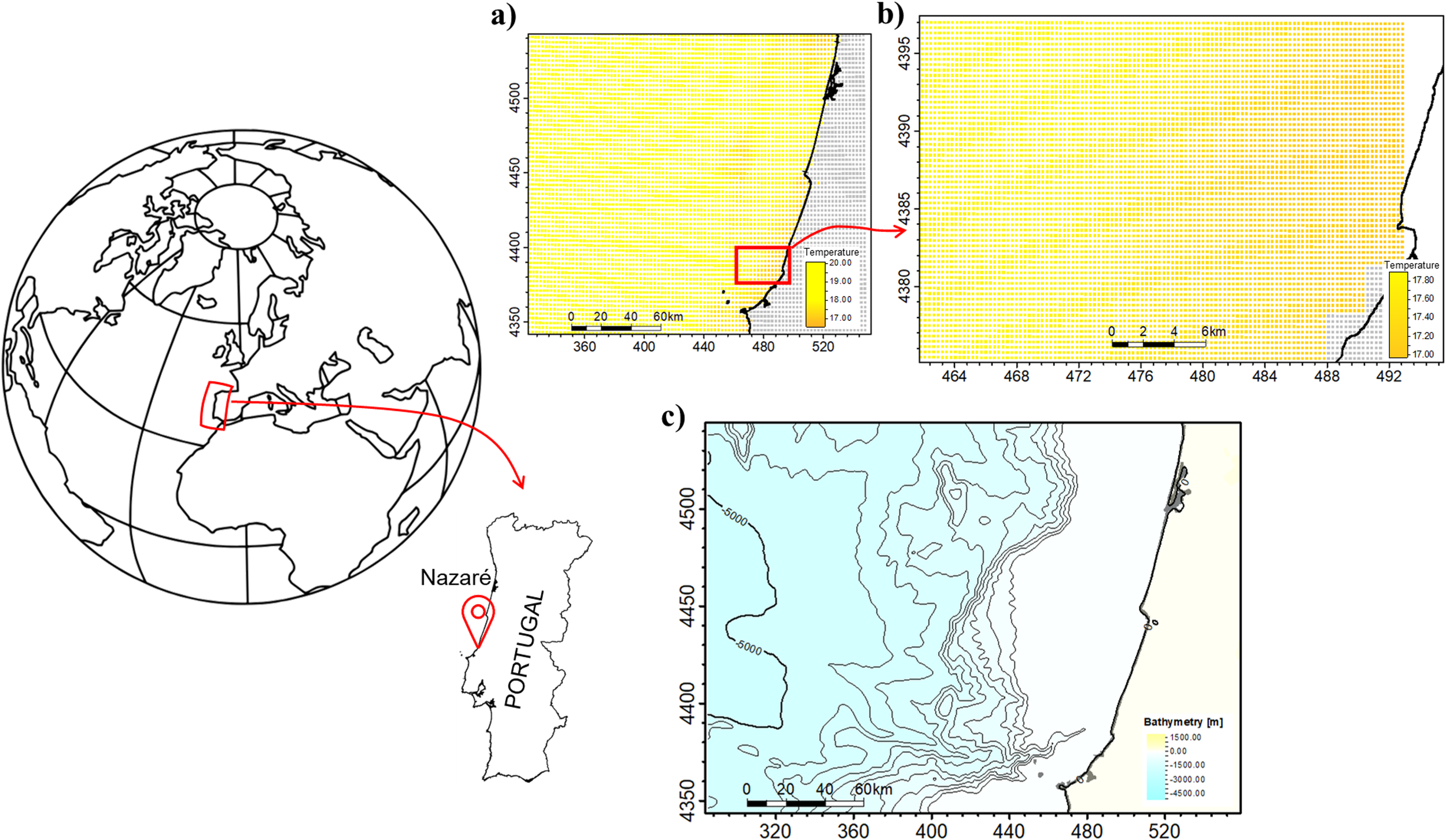
Figure 1. Location of the oceanographic survey, offshore Nazaré (Portugal): (a) regional sea surface temperature extracted from Copernicus Marine Service (CMEMS), model Atlantic-Iberian Biscay Irish- Ocean Physics Analysis and Forecast (European Union-Copernicus Marine Service, 2017); and (b) the grid refinement through uniform resampling of the original sea surface temperature model (a)); (c) the bathymetry of the region of interest. Coordinate reference system: WGS 84/UTM zone 29N.

In the next section, we describe in detail the proposed methodology to assimilate direct observations of ocean temperature acquired by AUVs and how to update spatial uncertainty maps. Then, in Section 3, we show the results obtained in the FRESNEL survey. Section 4 presents the results obtained and discusses and explores potential pathways for the proposed methodology. The last section summarizes the main conclusions of this work.

2 Methodology

The proposed methodology uses geostatistical simulation (i.e., direction sequential simulation (Soares, 2001) to predict three-dimensional models of ocean temperature and corresponding spatial uncertainty. The predictions are short-term, for a relatively small number of consecutive days, but they use limited computational resources and avoid running full numerical models of ocean dynamics. The temperature predictions are based on pre-existing, calibrated deterministic numerical models of ocean dynamics, which extend up to a certain day before the survey starts (or the day of interest). Figure 2 summarizes the proposed methodology, described in the subsequent sub-sections.

Figure 2

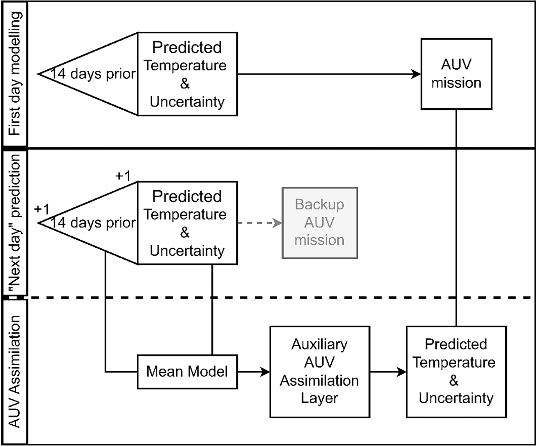
Figure 2. Schematic representation of the proposed methodology.

2.1 Geostatistical prediction of ocean temperature

In stochastic sequential simulation (Deutsch and Journel, 1998) all cells of a numerical model, represented by a grid, are sequentially visited following a random path. At each location along the random path, the kriging estimate and variance computed jointly from observed data (i.e., in situ measurements) and previously simulated grid cell locations within a neighborhood are used to define a probability distribution function of the variable of interest from which a value is drawn. As each run considers a different random path, and therefore the conditioning data is modified along the simulation path, it results in diverse predictions (i.e., geostatistical realizations). Different stochastic sequential simulation methods exist and differ in their a priori assumptions (Deutsch and Journel, 1998). In the proposed methodology, we use direct sequential simulation (Soares, 2001) (detailed in Appendix I) due to its flexibility and the ability to use the observed data directly without any Gaussian transform. In direct sequential simulation, the kriging estimate and kriging variance are computed following a spatiotemporal covariance matrix represented by a variogram model fitted to the experimental variogram, often computed from observations. In the field application show below we use a variogram model fitted to the CMEMS data due to their spatially exhaustive nature. The imposed spatiotemporal continuity model (i.e., covariance matrix) is an a priori assumption about the natural phenomena being modelled and exactly reproduced in all geostatistical realizations within a given ensemble of models.

The proposed methodology starts by retrieving the expected spatiotemporal continuity pattern for ocean temperature based on the a priori information provided by a deterministic calibrated ocean model for the study area over a long period (Figure 3a). These data are used to explore and model the spatiotemporal continuity pattern (i.e., directions of maximum spatiotemporal continuity). In the proposed methodology, the horizontal dimension represents the geographical coordinates of the numerical model of ocean dynamics (i.e., a deterministic model), while the vertical direction represents the temporal evolution of the model at a given depth. Specifically, the long-term calibrated ocean temperature is collated at each depth of the ocean numerical model (Figure 3a). Then, the three-dimensional experimental variogram is computed and fitted with a model. The range of the fitted variogram model along the vertical direction represents the maximum temporal continuity expected at that specific depth, and the horizontal range its spatial extent. The spatial analysis continues by repeating this process for the next depth of the numerical model of ocean dynamics (or down to the depth of interest). The independent variogram model per depth sample simultaneously capture of the spatiotemporal distribution of ocean temperature.

Figure 3

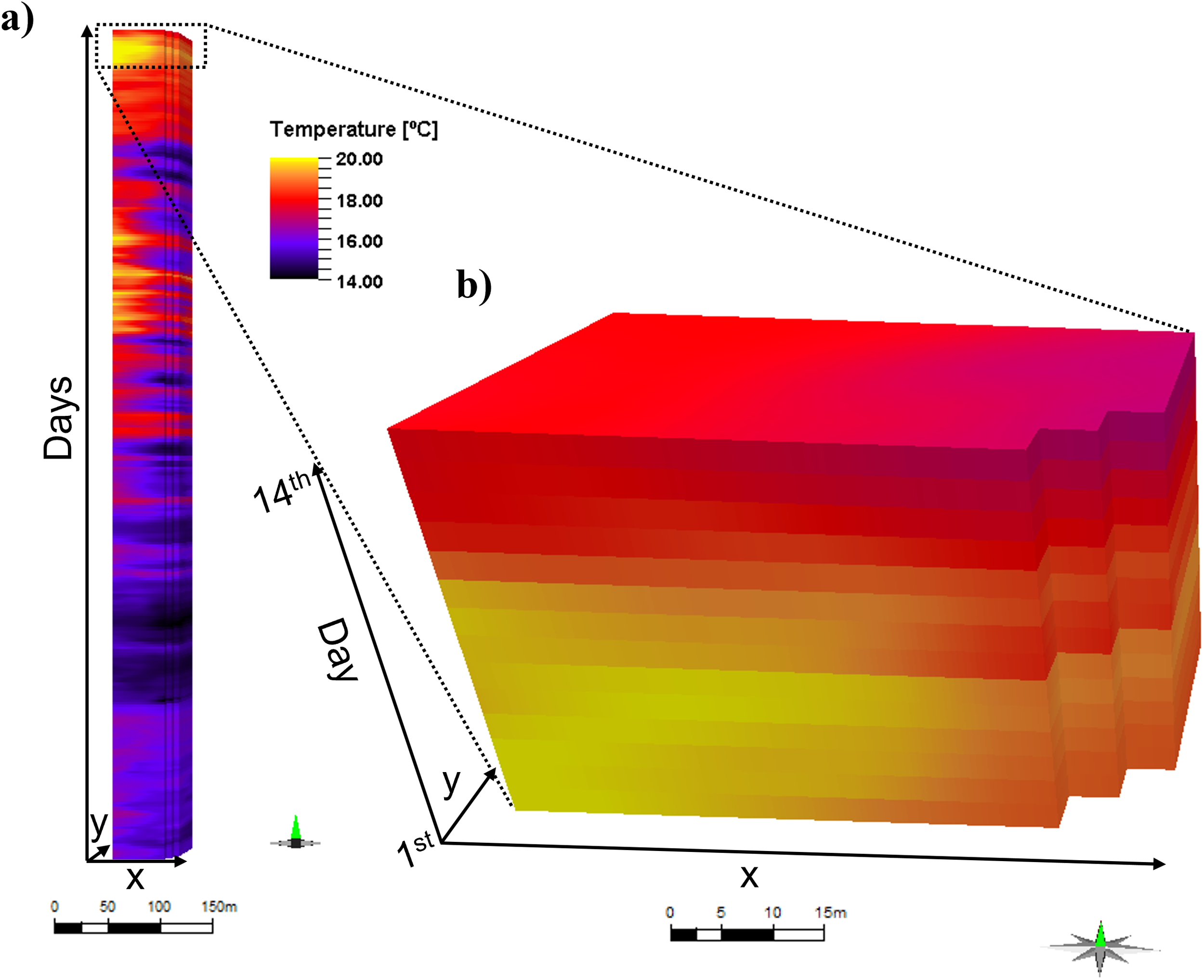
Figure 3. (a) Ocean temperature predicted from a calibrated deterministic temperature model for a given depth considering a long temporal window (i.e., one year). Each layer represents a given day in the long-term prediction; (b) for the same depth, zoom-in of the most recent fourteen consecutive days predicted by the deterministic model. This information is used to predict the subsequent one in the application example shown herein.

To forecast ocean temperature at a given depth, we use a set of fourteen previous days from the deterministic calibrated ocean model as observations while predicting the subsequent day (Figure 3b). Hence, the simulation grid is composed of a given number of layers as represented by the a priori data (i.e., the calibrated ocean model), followed by the layer corresponding to the forecasting day. Alternatively, additional a priori days might be considered depending on the oceanographic complexity of the study area. The selection of the grid size will mainly affect the computational cost of the simulation. After trial and error, and considering the study area specification, we opted for fourteen days, as this number allows for an efficient prediction of the subsequent day within a reasonable computational cost that could eventually be supported on-board by an AUV. Due to computational limitations, each depth of the numerical model is independently simulated. The described procedure is then applied to each depth of interest.

Multiple runs of the geostatistical simulation generate multiple geostatistical realizations of ocean temperature. The ensemble of geostatistical realizations approximates the posterior distribution of the predictions. It can be analyzed to assess the spatial uncertainty and variability of ocean temperature predictions. The spatial uncertainty maps can be obtained by computing the pointwise inter-quartile distance, or standard deviation, within the ensemble of geostatistical realizations. The predicted uncertainty maps enable the identification of areas that are more complex and/or less characterized, and can be used for intelligent path planning algorithms where high-uncertainty regions have higher rewards.

2.2 Data assimilation and stochastic model update

Besides predicting spatial uncertainty models for AUV path planning, the proposed geostatistical framework allows the seamless integration of direct measurements acquired by an AUV during an oceanography campaign. The data acquired on a given day of the oceanographic survey updates the ocean temperature forecast for the subsequent day. At this stage, we aim to predict the ocean temperature for the next day by combining previous predictions with newly measured data. In this case, the simulation grid is defined with only two layers (i.e., time steps). The first layer corresponds to the direct measurements of the AUV at its corresponding spatial location, and the second layer comprises the time step at which the new prediction will occur. As the spatial sampling of the AUV is frequently larger than the spatial resolution of the simulation grid, the data values that fall into the same cell are averaged to accommodate for resolution differences. In other words, we use a simple arithmetic upscaling between the AUV measurements and the grid cell value. Alternative methods could be applied depending on the objectives of the oceanographic survey (e.g., select the most extreme measurement for the upscaling). In highly heterogeneous areas (e.g., front regions) gradient-aware upscaling methods might produce more robust results. To incorporate the spatiotemporal patterns of the predictions for the day when the direct measurements were obtained, we use stochastic sequential simulation with local means (Soares, 2001) at the time step corresponding to the data acquisition. In direct sequential simulation with local means, the simulated value is based on its conditional distribution, considering previously simulated values, sample data and the local expected value as represented by the local mean model. This approach enables the update of the entire ocean model while simultaneously incorporating direct AUV measurements and previous a priori knowledge.

By incorporating these data sources, the simulation captures spatial trends and patterns that might otherwise be overlooked. It allows us to integrate new measurements without losing the overall spatial features obtained during the first step. The uncertainty of these predictions can be assessed as previously described (e.g., by computing the pointwise inter-quartile distance, or standard deviation, from a set of geostatistical realizations).

The temperature and spatial uncertainty predictions, obtained with the proposed methodology, are then used for intelligent path planning of AUVs and are sequentially updated based on the direct measurements acquired by AUVs during the oceanographic survey. The adaptive sampling algorithm (Bernacchi et al., 2025) concentrates measurements on locations with higher uncertainty as predicted by the ensemble of geostatistical realizations (i.e., spatial uncertainty maps). The use of this geostatistical simulation method allows to assimilate the direct observations and stochastically update the a priori models.

3 Field demonstration

The proposed methodology was tested and validated in a field oceanographic survey off W. Portugal (Figure 1) during the FRESNEL campaign for the last two weeks in October of 2024. The campaign aimed to test the autonomous maritime robots’ capacity to sample the ocean water, adapting their path based on the predictive models’ outputs, and to assimilate the acquired data for the subsequent predictions. The campaign involved the simultaneous deployment of multiple assets, including three Light Autonomous Underwater Vehicles (LAUVs) developed and operated by the Underwater Systems and Technology Laboratory (LSTS), University of Porto. The AUVs were equipped with conductivity, temperature, and depth (CTD) sensors that sampled the water from the surface until a depth of approximately 40 meters (to a maximum of 100 meters in specific cases where the bathymetry allows) following a “yo-yo” descending-ascending movement.

3.1 Data

The deterministic numerical model of ocean dynamics used to conditioning the geostatistical simulation was downloaded from the Copernicus Marine Service (CMEMS), model Atlantic-Iberian Biscay Irish- Ocean Physics Analysis and Forecast (European Union-Copernicus Marine Service, 2017), covering an area from 11.75°W to 8.43°W and from 39.00°N to 41.16°N with horizontal resolution of 0.028° in both directions, approximately 2.37km and 3.09km in x and y, respectively (Figure 1a), at Nazaré latitude. Vertically, the model has 17 depth samples, with decreasing vertical resolution with depth, covering from the sea surface to a depth of 40 meters. Temperature prediction is performed for each of these depth samples individually and independently. Since the spatial resolution of the AUV measurements is much higher than the deterministic CMEMS model, we increased the model grid spatial resolution eight times, by uniformly resampling the original grid, to better discretize the data to be assimilated throughout the grid model (Figure 1b). We applied the proposed methodology considering October 29th, 2024 as acquisition day, to predict the next day (i.e., October 30th, 2024).

3.2 Results

On the first survey data (October 29th, 2024), ocean temperature predictions and spatial uncertainty models were generated using information from the 14 previous days of the CMEMS product for the study area. This step yields seventeen 3-D datasets (i.e., one per depth sample considered), where the horizontal dimensions represent the x and y coordinates of the study area, and the vertical dimension represents the time step (i.e., a day). The CMEMS information was used as experimental data to model the three-dimensional variogram models at each depth sample and to constrain the geostatistical simulation of 100 realizations per depth. Figure 4 shows the resulting temperature and corresponding spatial uncertainty represented by the pointwise median (Figure 4a) and standard deviation (Figure 4b) computed from the ensemble of 100 geostatistical realizations, respectively. This information was used to select the deployment location and to define the AUVs’ path planning (Bernacchi et al., 2025) on the first day of the survey (Figure 4c).

Figure 4

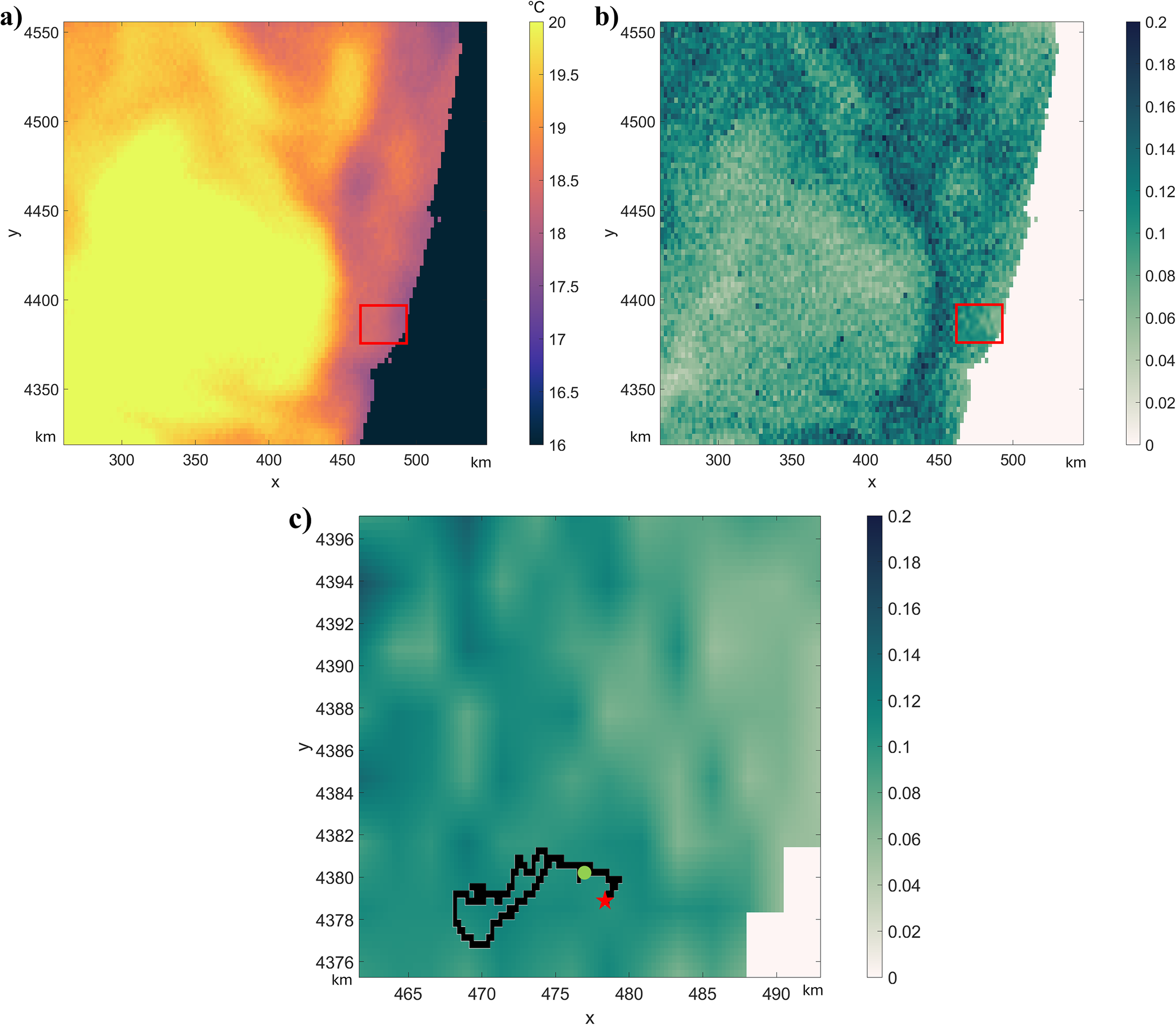
Figure 4. (a) Predicted pointwise median temperature models for the deployment day; (b) the corresponding uncertainty represented by the pointwise standard deviation. The red rectangle represents the refined grid location for deployment and study area; and (c) AUV path projection (black trajectory) at the sea surface (green circle representing start and red star the end of the path). Coordinate reference system: WGS 84/UTM zone 29N.

After deployment and AUV recovery, the measured temperature values at their corresponding coordinates and depths were upscaled to fit into the refined model grid. In general, the CMEMS model over predicts the ocean temperature measurements acquired by the AUV, with its performance decreasing with depth (Figure 5). Also, the range of AUV temperature measurements per grid cell increases with depth. This effect is expected as the vertical size of the CMEMS model grid cells increases with depth, allowing for more AUV samples per grid cell.

Figure 5

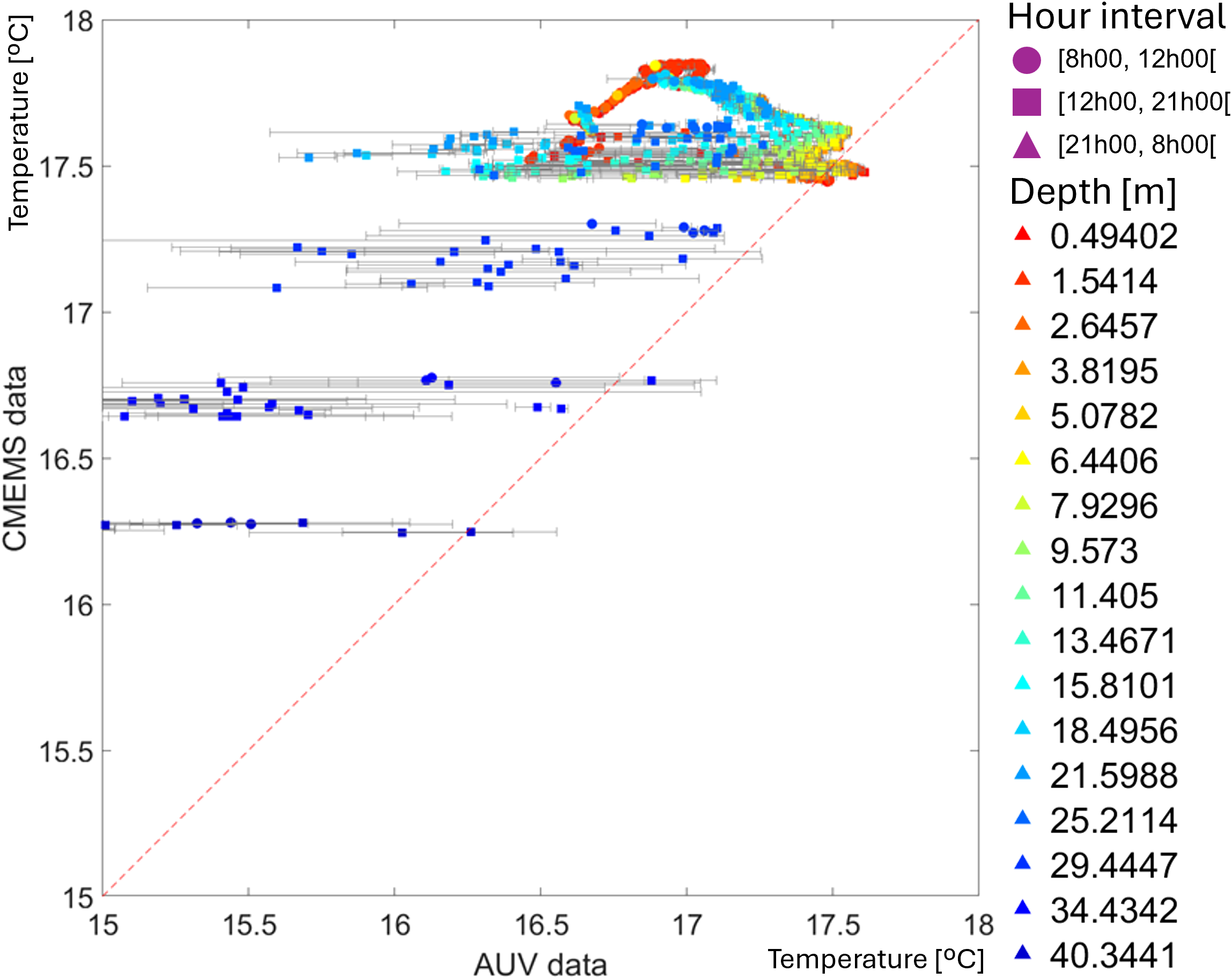
Figure 5. Comparison between temperature values from the CMEMS numerical model and the in-situ measurements from the AUV. Filled squares represent the mean of all AUV measurements within a model grid cell. The gray lines represent the range of measurements taken by the AUV. Depth in meters.

The upscaled temperature values were then assimilated into the models as conditioning data for predicting ocean temperature and spatial uncertainty for the next day.

3.3 Assimilation of temperature values and prediction

To highlight the importance of data assimilation and model update in obtaining more reliable short-term predictions, we begin by illustrating the temperature and spatial uncertainty predictions without AUV data assimilation for the next day (October 30th, 2024). Figure 6 illustrates temperature predictions based exclusively on the 14 days prior to the prediction day, CMEMS data, and does not consider any in-situ data. The pointwise median of 100 geostatistical realizations of temperature (Figure 6a) shows higher temperature values to the west of the model than in the opposite direction. The same region is characterized by high spatial uncertainty values (Figure 6b).

Figure 6

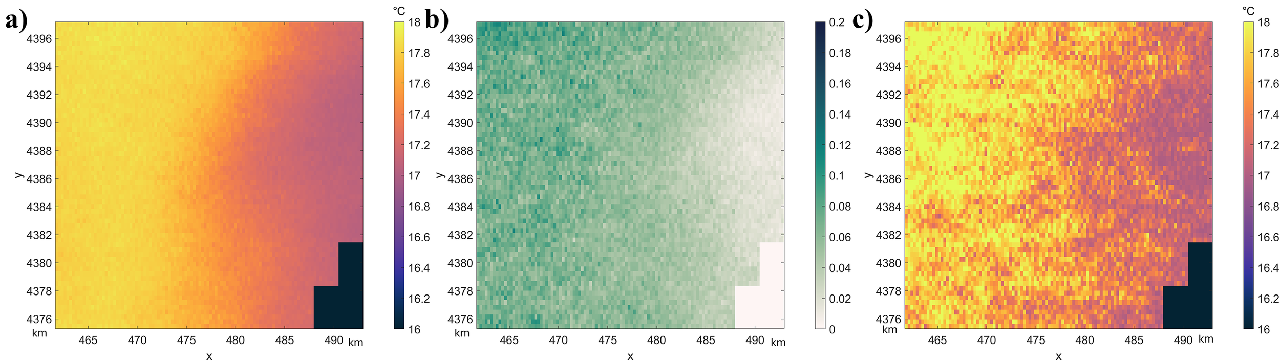
Figure 6. Next day prediction without assimilation of the AUV measured data, coordinate reference system: WGS 84/UTM zone 29N. (a) Pointwise median model predicted temperature, (b) uncertainty calculated with pointwise standard deviation, (c) one geostatistical realization of temperature.

The next day’s predictions after assimilation of the temperature values measured by the AUV are shown in Figure 7. The main spatial patterns of temperature are similar to those obtained without the assimilation (Figure 6), as the geostatistical simulation includes the a priori information provided by the calibrated oceanographic model for the survey area and the in situ measurements. However, the spatial uncertainty map (Figure 7b) changes considerably, illustrating the update of the a priori information with the data acquired during the survey. The highest temperatures (i.e., ~18°C) are located in the western part of the model. Still, the uncertainty values are low for the area surveyed by the AUV and larger in the opposite direction. Additionally, the predictions obtained from the CMEMS model are corrected to include colder water for the region sampled by the AUV (Figure 5).

Figure 7

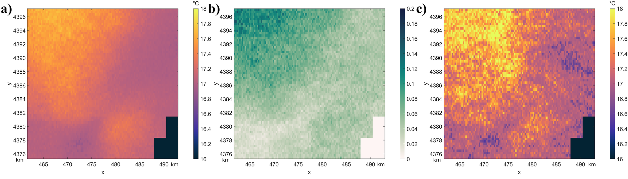
Figure 7. Next day prediction with assimilation of the AUV measured data. (a) Pointwise median model of predicted temperature, (b) uncertainty calculated with pointwise standard deviation, (c) one realization of temperature.

On October 30th, 2024, two different AUVs measured ocean temperature within the study area. One AUV followed a hand-planned navigation path, while the other used an automatically defined path planning over the three-dimensional spatial uncertainty model (Figures 8a, d). As we are not focused on the benefits and limitations of manual versus automatic AUV path planning, we assess the robustness of the data assimilation capabilities of the proposed methodology. Figure 8 shows the match between the direct measurements of both AUV versus the original CMEMS model and the updated one with the information collected on the previous day. The model update allows better predictions with higher match rates between the model and actual observations, allowing for compensation for the cold waters missing in the original CMEMS model.

Figure 8

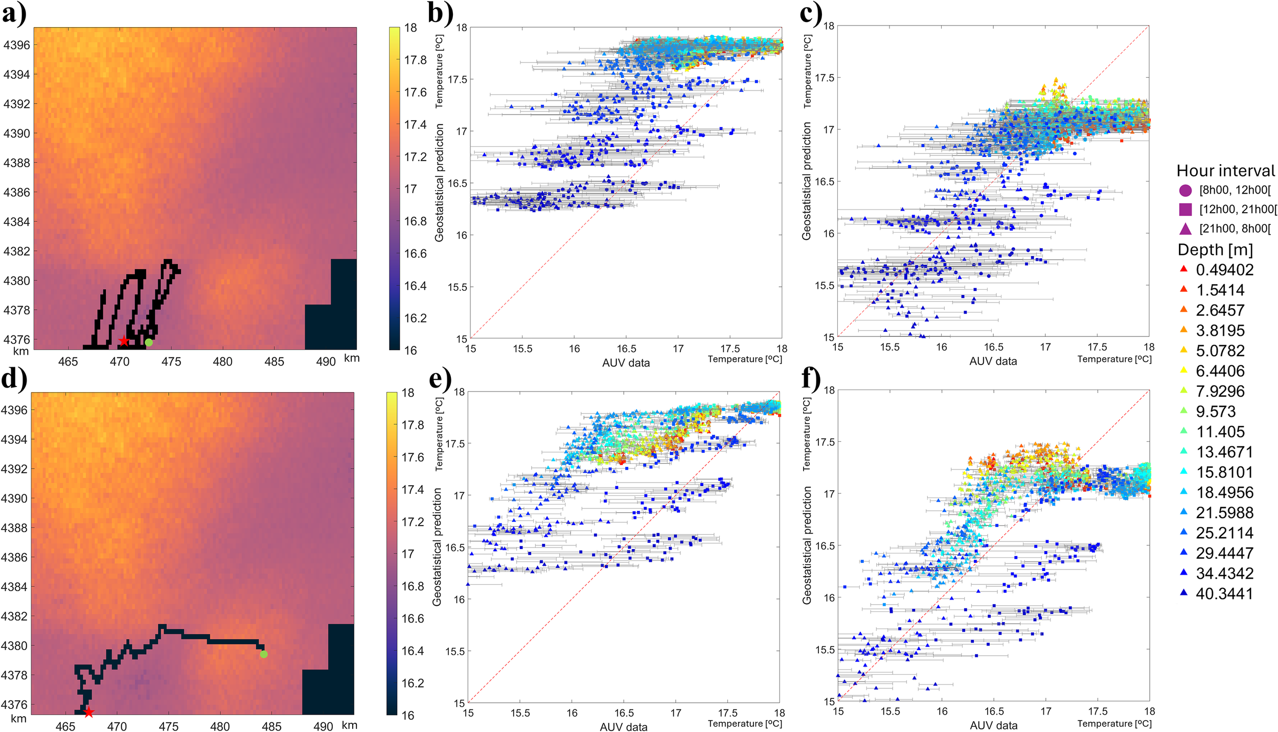
Figure 8. (a) LAUV-Xplore 5 path from the 30^th of Oct., and geostatistical temperature prediction for the same day after assimilation (green circle representing start and red star the end of the path). (b) Comparison of measurements and geostatistical model prediction for LAUV-Xplore 5 data location. (c) Comparison of measurements and geostatistical model prediction with AUV data assimilation from LAUV-Xplore 5 data location. (d) LAUV-Xplore 3 path from the 30^th of Oct., and geostatistical temperature prediction for the same day after assimilation (green circle representing start and red star the end of the path). (e) Comparison of measurements and geostatistical model prediction for LAUV-Xplore 3 data location. (f) Comparison of measurements and geostatistical model prediction with AUV data assimilation from LAUV-Xplore 3 data location.

4 Discussion

We proposed herein a geostatistical framework with a threefold objective. The first approach is to incorporate uncertainty into short-term predictions by utilizing full numerical models of ocean dynamics as conditioning data. The second objective is to assimilate direct measurements of ocean properties and update the initial ocean model. The third is to be computationally efficient, requiring low computational power aiming at the deployment of the proposed methodology in an autonomous vehicle for real-near-time data assimilation and model update.

The field application example demonstrates the capability of the predicted spatial uncertainty model to serve as input for an automatic AUV path planner. Areas associated with high spatial uncertainty are those where the calibrated deterministic numerical model of ocean dynamics exhibits more temporal variability, and therefore, mismatches between actual observations and predictions are expected. The application example illustrates an AUV navigation path through uncertain areas (Figure 4) and an overestimation of ocean temperature (Figure 5). The assimilation of the acquired data results in a change in the spatial uncertainty pattern (Figure 6, Figure 7), illustrating the impact of data assimilation on the prediction. Additionally, the data assimilation produces predictions that are closer to the actual observations (Figure 8), even for navigation paths that do not depend on the predicted spatial uncertainty.

While the geostatistical approach does not include any physical constraints in terms of oceanographic behavior, its computational costs are negligible when compared with full numerical models of ocean dynamics. The computational cost of a geostatistical realization depends exclusively on the number of grid cells that comprise the model covering area of interest. This aspect opens the door for the deployment of these methods in the AUV’s on-board processing unit, as well as for automatic data assimilation, model update, and spatial uncertainty prediction in near-real-time and data cycles shorter than those illustrated herein.

On the other hand, the quality of the prediction depends on the quality of the existing a priori ocean model and its resolution, as this information will be used as constraining data, as well as the ability to retrieve reliable variogram models from the existing historical data. Using an incorrect variogram model will decrease the quality of predictions and the usefulness of the proposed methodology, and a lower resolution may cause problems when identifying sub-mesoscale structures. Additionally, the independent prediction at each depth sample is a disadvantage, as it may overlook existing vertical dependencies. This aspect might be addressed with dimensionality reduction techniques as proposed in prediction problems related to geophysics (Azevedo, 2022) or with the development of a full spatiotemporal model. With the proposed approach the vertical dependencies are implicitly modelled by the a priori information used as data conditioning during the prediction.

Finally, the geostatistical framework enables a flexible approach. While the application example shown herein deals with ocean temperature, the property of interest could be any biogeochemical property if there are historical data for this property in the study area and sensors to measure it in the field. Given its low computational cost, the geostatistical model can also be implemented on-board the AUVs, allowing it to be updated more frequently with in situ data and to optimize operations on the fly using as priors to adaptive sampling algorithms.

5 Conclusions

In this work, we introduced a geostatistical modelling approach designed to support smart data collection and efficient trajectory planning for AUVs. By predicting ocean temperature and spatial uncertainty, the method qualifies AUVs to identify and prioritize regions where data collection would be most valuable. This targeted approach increases knowledge while reducing unnecessary exploration, ultimately enhancing the scientific return of oceanographic missions.

Although, this methodology can be applied as is to an oceanographic campaign, it would benefit from some upgrades such as using an a priori model with higher resolution, overcoming the necessity of increasing the resolution by interpolation. This will allow to better capture sub-mesoscale structures and interesting features to sample.

Due to the method’s ability to work with lightweight computations, making it well suited for real-time decision making in the field, the integration of the algorithm into the AUV during the deployment also brings autonomy to the sampling, and makes use of a more efficient path planning that have previous measurements in consideration and accommodates real-time conditions and unexpected changes in the environment.

Data availability statement

Publicly available datasets were analyzed in this study. This data can be found here: https://resources.marine.copernicus.eu/product-detail/IBI_ANALYSISFORECAST_PHY_005_001/INFORMATION.

Author contributions

AD: Conceptualization, Investigation, Methodology, Writing – original draft, Writing – review & editing. LB: Data curation, Methodology, Writing – review & editing. RM: Conceptualization, Data curation, Investigation, Methodology, Resources, Supervision, Validation, Writing – review & editing. JS: Conceptualization, Data curation, Investigation, Methodology, Resources, Supervision, Validation, Writing – review & editing. LA: Conceptualization, Investigation, Methodology, Supervision, Validation, Writing – original draft, Writing – review & editing.

Funding

The author(s) declare financial support was received for the research and/or publication of this article. LA and AD gratefully acknowledge the support of the CERENA (FCT/04028/2025). AD is funded by the Fundação para a Ciência e a Tecnologia (Portuguese Foundation for Science and Technology) through the project PRT/BD/154661/2023. JS and RM acknowledge the support of the LAETA within the scope of the project with reference UIDB/50022/2020. The authors acknowledge the FRESNEL project (Field expeRiments for modEling, aSsimilatioN and adaptive sampLing), funded by the Office of Naval Research (ONR) under ONR award number N00014-22-1-2796. The work was also supported by JUNO—Robotic Exploration of Atlantic Waters project—Ref^a 2021/0008—from FLAD, by the DiverSea project, supported by the European Commission under grant agreement 101082004 and the TRAINEE project (https://doi.org/10.54499/2024.07606.IACDC) supported by FCT.

Conflict of interest

The authors declare that the research was conducted in the absence of any commercial or financial relationships that could be construed as a potential conflict of interest.

Generative AI statement

The author(s) declare that no Generative AI was used in the creation of this manuscript.

Any alternative text (alt text) provided alongside figures in this article has been generated by Frontiers with the support of artificial intelligence and reasonable efforts have been made to ensure accuracy, including review by the authors wherever possible. If you identify any issues, please contact us.

Publisher’s note

All claims expressed in this article are solely those of the authors and do not necessarily represent those of their affiliated organizations, or those of the publisher, the editors and the reviewers. Any product that may be evaluated in this article, or claim that may be made by its manufacturer, is not guaranteed or endorsed by the publisher.

References

Azevedo L. (2022). Model reduction in geostatistical seismic inversion with functional data analysis. GEOPHYSICS 87, M1–11. doi: 10.1190/geo2021-0096.1

Crossref Full Text | Google Scholar

Bernacchi L., Duarte A. F., Mendes R., Azevedo L., and Sousa J. B. D. (2025). "Closing the Data Loop: Real-World AUVs Adaptive Sampling for Improved Ocean Model Predictions," 2025 Symposium on Maritime Informatics and Robotics (MARIS), Syros, Greece, 2025, pp. 1-8 doi: 10.1109/MARIS64137.2025.11139688

Crossref Full Text | Google Scholar

Deutsch C. V. and Journel A. G. (1998). GSLIB: geostatistical software library and user’s guide. Version 2.0. 2nd ed (New York: Oxford University Press), 1.

Google Scholar

European Union-Copernicus Marine Service (2017). Atlantic-Iberian Biscay Irish- Ocean Physics Analysis and Forecast (Mercator Ocean International). Available online at: https://resources.marine.copernicus.eu/product-detail/IBI_ANALYSISFORECAST_PHY_005_001/INFORMATION (Accessed February 11, 2025).

Google Scholar

Gafurov S. A. and Klochkov E. V. (2015). Autonomous unmanned underwater vehicles development tendencies. Proc. Engineering. 106, 141–148. doi: 10.1016/j.proeng.2015.06.017

Crossref Full Text | Google Scholar

Ge Y., Eidsvik J., and Mo-Bjørkelund T. (2023). 3-D adaptive AUV sampling for classification of water masses. IEEE J. Oceanic Eng. 48, 626–639. doi: 10.1109/JOE.2023.3252641

Crossref Full Text | Google Scholar

Gould J., Sloyan B., and Visbeck M. (2013). “In Situ Ocean Observations,” in International Geophysics (Elsevier), 59–81. Available online at: https://linkinghub.elsevier.com/retrieve/pii/B9780123918512000039 (Accessed March 31, 2025).

Google Scholar

Hwang J., Bose N., and Fan S. (2019). AUV adaptive sampling methods: A review. Appl. Sci. 9, 3145. doi: 10.3390/app9153145

Crossref Full Text | Google Scholar

Kite-Powell H., Colgan C., and Weiher R. (2008). Estimating the economic benefits of regional ocean observing systems. Coast. Management. 36, 125–145. doi: 10.1080/08920750701868002

Crossref Full Text | Google Scholar

Lermusiaux P. F. J. (2007). Adaptive modeling, adaptive data assimilation and adaptive sampling. Physica D: Nonlinear Phenomena. 230, 172–196. doi: 10.1016/j.physd.2007.02.014

Crossref Full Text | Google Scholar

Mahdavi S., Amani M., Bullock T., and Beale S. (2021). A probability-based daytime algorithm for sea fog detection using GOES-16 imagery. IEEE J. Sel Top. Appl. Earth Observations Remote Sensing. 14, 1363–1373. doi: 10.1109/JSTARS.2020.3036815

Crossref Full Text | Google Scholar

Mendes R., Da Silva J. C. B., Magalhaes J. M., St-Denis B., Bourgault D., Pinto J., et al. (2021). On the generation of internal waves by river plumes in subcritical initial conditions. Sci. Rep. 11, 1963. doi: 10.1038/s41598-021-81464-5

PubMed Abstract | Crossref Full Text | Google Scholar

Minnett P. J., Alvera-Azcárate A., Chin T. M., Corlett G. K., Gentemann C. L., Karagali I., et al. (2019). Half a century of satellite remote sensing of sea-surface temperature. Remote Sens. Environment. 233, 111366. doi: 10.1016/j.rse.2019.111366

Crossref Full Text | Google Scholar

Mo-Bjørkelund T., Mendes R., López-Castejón F., and Ludvigsen M. (2025). Adaptive ocean gradient tracking using an autonomous underwater vehicle with a boundless model. IEEE J. Oceanic Eng. 50, 955–967. doi: 10.1109/JOE.2024.3484577

Crossref Full Text | Google Scholar

O’Carroll A. G., Armstrong E. M., Beggs H. M., Bouali M., Casey K. S., Corlett G. K., et al. (2019). Observational needs of sea surface temperature. Front. Mar. Sci. 6, 420. doi: 10.3389/fmars.2019.00420

Crossref Full Text | Google Scholar

Paull L., SaeediGharahbolagh S., Seto M., and Li H. (2012). “Sensor driven online coverage planning for autonomous underwater vehicles,” in 2012 IEEE/RSJ International Conference on Intelligent Robots and Systems (IEEE, Vilamoura-Algarve, Portugal), 2875–2880. Available online at: http://ieeexplore.ieee.org/document/6385838/ (Accessed March 31, 2025).

Google Scholar

Petillo S., Balasuriya A., and Schmidt H. (2010). “Autonomous adaptive environmental assessment and feature tracking via autonomous underwater vehicles,” in Oceans’10 Ieee Sydney (IEEE, Sydney, Australia), 1–9. Available online at: http://ieeexplore.ieee.org/document/5603513/ (Accessed March 31, 2025).

Google Scholar

Pinto J., Mendes R., Da Silva J. C. B., Dias J. M., and De Sousa J. B. (2018). “Multiple Autonomous Vehicles Applied to Plume Detection and Tracking,” in 2018 OCEANS - MTS/IEEE Kobe Techno-Oceans (OTO) (IEEE, Kobe), 1–6. Available online at: https://ieeexplore.ieee.org/document/8558802/.

Google Scholar

Sloyan B. M., Wilkin J., Hill K. L., Chidichimo M. P., Cronin M. F., Johannessen J. A., et al. (2019). Evolving the physical global ocean observing system for research and application services through international coordination. Front. Mar. Sci. 6, 449. doi: 10.3389/fmars.2019.00449

Crossref Full Text | Google Scholar

Soares A. (2001). Direct sequential simulation and cosimulation. Math. Geology. 33, 911–926. doi: 10.1023/A:1012246006212

Crossref Full Text | Google Scholar

Teixeira D., Sousa J. B. D., Mendes R., and Fonseca J. (2021). “3D Tracking of a River Plume Front with an AUV,” in OCEANS 2021: San Diego – Porto (IEEE, San Diego, CA, USA), 1–9. Available online at: https://ieeexplore.ieee.org/document/9705995/ (Accessed February 6, 2025).

Google Scholar

Toth P. and Vigo D. (Eds.) (2002). The Vehicle Routing Problem ed Toth P and Vigo D (Philadelphia: Society for Industrial and Applied Mathematics). doi: 10.1137/1.9780898718515

Crossref Full Text | Google Scholar

Yu F., He B., Liu J., Wang Q., and Shen Y. (2022). Towards autonomous underwater vehicles in the ocean survey: A mission management system (MMS). Ocean Engineering. 263, 111955. doi: 10.1016/j.oceaneng.2022.111955

Crossref Full Text | Google Scholar

Zhang Y., Godin M. A., Bellingham J. G., and Ryan J. P. (2012). Using an autonomous underwater vehicle to track a coastal upwelling front. IEEE J. Oceanic Eng. 37, 338–347. doi: 10.1109/JOE.2012.2197272

Crossref Full Text | Google Scholar