To heat or to heal: the uneasy trade-off between energy and healthcare expenditure in Central Asia

The influence of housing hazards on healthcare has become a serious problem, considering the past and present implications of international energy laws. In this empirical study, energy poverty was examined to reveal its impact on health-oriented spending in Tajikistan for the year 2013. Our analysis demonstrated the negative effect of fuel poverty on healthcare expenditure across different income groups. The findings indicated that families with high and middle incomes experience a low level of energy poverty, suggesting that the health expenses of households from these income classes are not impacted by energy poverty levels. The low-income group, however, is considered to be fuel-poor, with an energy poverty level prevailing at 10%. Nevertheless, families in the very low-income group live in extreme fuel poverty, spending nearly half of their budget on fuel expenditure. The results provide evidence that fuel poverty negatively affects health and that this effect is deferred, leading to poorer health over time. This paper also investigates the impact of fuel expenditure on healthcare spending, revealing a negative correlation between the two observed variables. The model is controlled for dwelling size, location of housing, and dwelling type, which demonstrate a significant impact on healthcare expenditure. Additionally, household size was found to be highly statistically significant at a 95% confidence interval, holding all other factors constant. Regarding policy, this paper highlights the importance of investments in housing energy schemes to increase efficiency and decrease fuel poverty, thereby improving health indicators. It suggests that conditions in households that reduce fuel poverty can drive down public healthcare costs. The results indicate that the very low and low-income groups experience proportionally higher healthcare expenditure due to fuel poverty, underscoring the necessity for policy intervention.

Introduction

Economic poverty is a harsh reality for citizens of many countries, including Tajikistan, regardless of the rapid economic growth in some countries and governmental programs aimed at improving the situation. The situation worsens as poverty, especially energy poverty, prevents people from pursuing education and job opportunities, further exacerbating health issues. Therefore, the development of better socio-economic conditions relies on clean, affordable, and reliable energy sources. The United Nations has established 17 Sustainable Development Goals to organize universally accessible energy in modern society, emphasizing the need for affordable and sustainable energy by the year 2030 (United Nations, 2019). Specifically, addressing SDG 1, which stands for “No Poverty,” and SDG 3, “Good Health and Wellbeing”, highlights the interconnectedness of sustainable development goals.

Energy poverty must be addressed because interrupted electricity disrupts medical equipment, making it nearly impossible for hospitals to operate continuously and effectively. The right to live a healthy life is a fundamental human right that is being compromised by institutions specifically created to save lives; this right is neglected due to poverty.

This study aims to reveal the impact of fuel poverty on healthcare expenditure, based on socioeconomic factors such as gender, dwelling size, and household location as control variables. Researchers Boardman (1991) and Bouzarovski (2014) have established a link between energy poverty and household wellbeing. More recent studies by Du and Zhang (2025) and Ucal and Günay (2022) have highlighted the effect of energy poverty on mental health and happiness levels.

In addition, without reliable electricity, people lack access to household appliances that aid their education and professional growth, such as the internet, computers, TVs, and radios. This decreases citizens' chances for a better socioeconomic status by hindering effective learning and career choices.

Economically, high costs of electricity and energy disproportionately affect low-income households, worsening poverty and lowering living standards. Even the business day may be impacted by power shortages and the poor health conditions of workers who cannot afford medical treatment and whose health deteriorates due to a lack of electricity. Such households often resort to using fossil fuels and other pollutants, putting their health at risk while indoors.

Hence, the aim of this study is to investigate the effect of energy poverty on the socio-economic factors of households. At the same time, household energy deficiency is becoming a more widespread issue in post-Soviet Central Asian countries due to two principal reasons: (i) a trap in the transition from a centrally-planned to a market-based economy, lacking cost-reflective tariffs for utilities that would enable financial sustainability; and (ii) insufficient investments in operating and maintaining the inherited Soviet-era, inefficient, and loss-prone infrastructure for electricity, natural gas, heating, and water supply. This centrally-supplied energy deficiency problem is particularly acute in remote rural areas, where the proportion of the low-income population is higher.

In the case of energy poverty, rural households face an anxious trade-off between spending their limited income on alternative fuels for heating, cooking, hot water supply, and electricity generation (in the form of coal, firewood, LPG, or gasoline) or benefiting from paid healthcare services. In majority of cases, individual patients' healthcare interests are sacrificed in favor of the entire family's energy-related needs.

Therefore, this study aims to investigate the effect of energy poverty on the socioeconomic factors of households:

• Gender

• Nominal monthly fuel expenditure

• Dwelling size

• Location of housing: rural/urban

• Type of heating appliance

• Number of household members

• Dwelling type: multistory,

• Household hazards

• Consumption of seasonal utilities—hot and cold water, electricity, wastewater, natural gas supply, waste collection

Consequently, the study sets the following objectives: (i) investigate the relationship between health-related issues and fuel poverty (instrumental variable, control: type of appliance used by households for heating); (ii) determine the impact of fuel expenses on healthcare expenses; and (iii) clarify the relationship (nexus) between fuel poverty and health expenditure in rural and urban areas.

As a result, the current study reveals the effect of energy poverty on healthcare expenditure in the context of Tajikistan. Its results and findings can be generalized to the rural areas of Kyrgyzstan and Uzbekistan, where socioeconomic setups and indicators, as well as the overall condition of the centrally supplied energy infrastructure, are similar.

Literature review

Access to energy is crucial for modern household sustainability, which is negatively affected by energy poverty. According to Kanagawa and Nakata (2018), limited access to clean energy and lack of affordability for poor households can worsen the health conditions and education levels of household members. These effects are especially detrimental for women and children, who spend relatively more time indoors and are often responsible for household chores in countries with lower access to energy. For instance, in Assam, India, it was found that the literacy rate could be improved from 63% to 74% through complete electrification.

The concept of fuel poverty is based on an energy requirement, as modeled by Hills (2012), which indicates that energy use in the household does not affect the modeled energy use requirements. This means that it does not influence the household's fuel poverty status. This holds true for both determinants: current and proposed LIHC indicators, as both use similar evaluations of household energy based on a model.

In addition to other adverse effects of energy poverty, limited access to proper sources of electricity can lead to illegal actions by citizens. For example, members of households without electricity may attempt to “pilfer electricity” from public lines, recognizing the importance of access to electricity, which in turn exacerbates public access issues. Raghavan (2018) stated that energy theft is a major cause of distribution losses in India, where energy theft accounts for almost 60% in some states.

Housing hazards are environmental hazards and are essential indicators of health. They relate to any risks to household members' health and safety resulting from deficiencies (Kahouli, 2020). Kahouli states that the first area of focus in this paper will be the effects of household conditions on health. Further, the emphasis will be on fuel poverty housing hazards, which is a more specific case. This paper consists of two types of studies: analyzing the effects of household conditions on health, including and extending beyond the influence of fuel poverty, and focusing on the effects of fuel poverty on health.

According to Ranjan and Singh (2017), the costs of installing and setting up an electric connection are often prohibitively high for majority of households in rural areas; however, if the initial installation costs are subsidized, households might still be able to cover their monthly electricity bills, which would mark progress for rural areas in many countries with limited energy access.

On the contrary, a study by Banerjee et al. (2015) for the World Bank suggests that low-income populations may still struggle to afford monthly electricity costs even if installation is subsidized. They argue that this assumption may lack validity, as those households' expenditures on unclean energy sources, such as kerosene, are usually comparable to the costs of electric services. For context, electricity was found to be affordable in India, where even for low-income households, electric services accounted for 3.4% of the average budget in 2010.

Sharma (2019) reported that variations in monthly electricity bills usually result from independent variables such as household income, appliance usage, family size, dwelling size, time spent outdoors, the stock of appliances, and education level.

UNDESA (2014) revealed that nearly 27% of schools in villages in India lack reliable access to energy. In addition, lack of electricity access in households disrupts the studying process and school attendance. Students from families with electricity access tend to perform better in school and achieve greater success later. Electrified households demonstrated significantly better literacy rates, and schools with electricity experienced enrollment increases of 6% for boys and 7.4% for girls.

Furthermore, the consumption of unclean cooking fuels, together with kerosene, coal, firewood, and cow dung cake, along with the use of inefficient stoves, poses significant risks for the population as it results in emissions and air pollution from carbon monoxide and nitrogen oxides. This condition can have negative effects on health, including fatal cases (Kanti, 2017). Limited access to energy can lead to malnutrition and cardiovascular diseases and may hinder overall individual development. Additionally, traditional energy sources for heating and cooking cause more than 400,000 premature deaths of women and children in India yearly (World Health Organization, 2014).

One of the biggest sources of heating and cooking energy, kerosene, creates hazardous combustion when used indoors without proper ventilation. The results of such practices pose significant health risks, including but not limited to pulmonary disorders and skin ailments. The byproducts of kerosene also contribute to black carbon emissions. The conditions of most low-income households' appliances are so inefficient that they require large purchases of kerosene, resulting in substantial indoor emissions and environmental damage. In India, government subsidization of kerosene leads to perverse consumption patterns, despite the alarming health and environmental effects.

Baker (2001) researched the relationship between health risks and residing in a household experiencing fuel poverty. The research suggested a strong link between decreased temperatures inside the house and an increased risk of stroke, heart attack, and respiratory illnesses. Furthermore, there is evidence of a link between cold stress and cardiovascular strain, with increasing cases of dust mites in poorly ventilated houses, leading to asthma and eczema. This is especially concerning for children in such households. There is also evidence that mold and dampness present in homes negatively affect the physical and mental health of household members (Baker, 2001).

According to Sharma (2019) and Owoundi (2013), there is a correlation between energy poverty and income poverty. Additionally, pollution influences health issues that arise from energy poverty. Therefore, positive changes and developments in one variable can help improve other variables and vice versa.

Various methodologies and approaches, such as panel data or instrumental variables, can be applied to analyze the impact of fuel poverty.

In this context, the Ordinary Least Squares (OLS) regression model has proven its validity and effectiveness in quantifying the contribution of energy poverty to healthcare. The standard form of the OLS model enables researchers to interpret the coefficients for energy/fuel poverty alongside additional control variables, indicating the magnitude as well as the direction of its effect on health. The estimated coefficients for fuel poverty could provide quantitative evidence of public wellbeing. A statistically significant positive or negative coefficient indicates whether energy poverty worsens or improves healthcare outcomes.

The studies by Pan (2020) and Davillas et al. (2023) emphasize the significance of the OLS model in understanding this nexus. Pan (2020) apply OLS regression to analyze the effect of energy poverty on global public healthcare. The authors highlight the fundamental assumptions for the OLS regression model, such as homoscedasticity, linearity, and absence of multicollinearity between explanatory variables. The paper uses energy poverty as an independent variable and multiple health-related outcomes, such as disease prevalence and life expectancy, as dependent variables. The model also accounts for economic conditions through control variables such as GDP per capita and level of education, which allows for the isolation of energy deprivation's impact on public wellbeing. The study underscores the direct negative impact of energy poverty on public health due to limited access to energy sources, resulting in negative health outcome contributors such as poor air quality and inadequate heating.

Similarly, Davillas et al. (2023) examine the effects of fuel poverty on objective (physical health) and subjective (self-reported health) wellbeing measures by applying the OLS model. While Pan et al. analyze energy poverty on a macro scale, Davillas et al. (2023) study fuel poverty on a more granular level, focusing on households struggling to meet basic energy needs for heating. The paper adds to the growing evidence of energy poverty's adverse impact on health metrics, especially among low-income and middle-income groups in countries with limited access to energy.

Although both research papers focus on various yet complementary aspects of energy poverty, they share effective implications of OLS to analyze a linear relationship between energy/fuel poverty and health while encountering potential limitations. Pan (2020) raise concerns regarding endogeneity and omitted variable bias while highlighting the possible occurrence of reverse causality between energy poverty and public wellbeing. Similarly, Davillas et al. (2023) address the challenge of adverse causality, where poor health conditions could trigger fuel poverty. Both papers suggest a deeper evaluation of these issues, noting that unobserved factors could influence both outcomes, through the application of more advanced econometric tools, such as instrumental variables.

Methodology

The current paper examines several socio-economic variables (SEVs) of households (HHs) to investigate the HHs' level of fuel poverty. It is important to note that, although the government controls the technological side of the energy sector, social factors are beyond its control, highlighting the significance of this research.

The framework conceptually considers the Energy Justice Theory to emphasize fairness in affordability regarding fuel/energy access for households. The concept of fuel poverty indicates a critical housing hazard with a direct impact on health outcomes, driving medical bills for financially vulnerable individuals. This study presents the following pattern: fuel poverty → highly limited energy access → thermal discomfort → higher medical risks → higher healthcare expenditures.

Data description

The paper analyzes the impact of fuel poverty on socio-economic determinants in the case of Tajikistan. This report applies cross-sectional data that gathers information for a particular point in time. Theoretically, a cross-sectional study is a strong approach to assessing the relationship between health-oriented issues and other aspects of interest (Gujarati and Porter, 2009). Thus, to evaluate the effect of energy poverty on healthcare expenditure, this study employed the Jobs, Skills, and Migration Survey dataset (CALISS HH TJ). It was obtained from the World Bank and the German Federal Enterprise for International Cooperation (GIZ), which was conducted in 2013 (World Bank, 2017). The survey includes 2,808 observations, examining all existing regions of Tajikistan: Dushanbe, Sogd, Districts of Republican Subordination, Khatlon, and Gorno-Badakhshan. The survey employed a designed questionnaire that was distributed among HHs. The questionnaire comprised a wide range of information on HH profiles, covering areas such as the labor market, health, fuel, food and non-food consumption, dwelling characteristics, budget, and so forth.

The data on HHs' total monthly income was sorted by indicated currencies, which included Tajik somoni (TJS), Russian rubles (RUB), and US dollars (USD). All currencies were converted to USD to standardize the data, using the 2013 average exchange rate of 4.76 TJS = 1 USD and 32.69 RUB = 1 USD (FxRates, 2020). Furthermore, according to Sharma (2019), the HHs were evenly separated into four income groups by frequency: high-income group (HIG), middle-income group (MIG), low-income group (LIG), and very low-income group (VLIG). Each of the income thresholds contained 702 observations. However, this method of grouping created double counting, with overlaps between the groups. Specifically, VLIG and LIG, as well as LIG and MIG, included households with identical amounts of total monthly income, leading to measurement errors that could bias results. To avoid such risks, the data was divided differently, grouping total monthly income by sums. After grouping the data following Sharma's method, it was observed that HHs with a total monthly income of 126 USD were classified under both VLIG and LIG. Hence, all HHs with an income of 126 USD were classified solely as VLIG. This adjustment is justified by the average number of household members, which was estimated to be five people in VLIG after adding the overlapping HHs, indicating a large family size. According to the International Labor Organization (2020), in 2013, the minimum wage in Tajikistan was 51.5 USD per worker. Thus, HHs with a monthly income of 126 USD effectively had 25.21 USD per household member, which is almost half the minimum monthly salary. This implies that the groups are formed logically, considering household sizes as well as monthly wages set by the government.

From Table 1, it can be observed that VLIG covers a minimum of 130.25 USD, LIG is constrained from 131.93 USD to 250 USD inclusively, while MIG ranges from 252 to 499 USD, and HIG includes incomes above 500 USD. The data became unbalanced due to the distinct number of observations in each income group. This will not cause biased results, as the number of observations does not vary significantly, and each group is to be observed separately.

Table 1

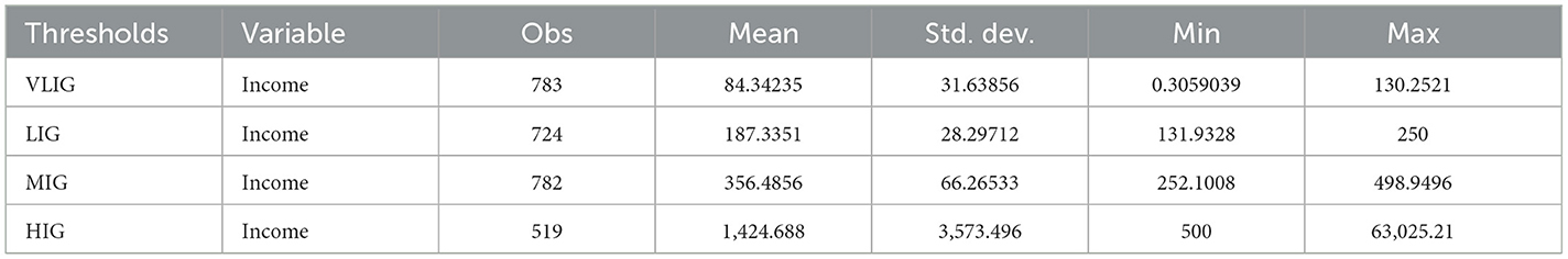
Table 1. Descriptive statistics of variable (income) by thresholds.

Methods

The analysis applies the consumption expenditure approach to investigate the level of fuel poverty among observed HHs. According to Hills, a household is considered energy poor if its total fuel expenses exceed 10 percent of its disposable income (2011). To estimate the energy poverty level in HHs, the following manipulations were conducted (Hills, 2011, 2012):

$\begin{array}{l}I=\frac{Equivalizedfuelcosts}{Equivaliseddisposableincome(beforehousingcosts)}\end{array}$

if I>10%, the HH experiences energy poverty

$\begin{array}{l}\text{Equivalized disposal income }=\frac{DisposalIncome}{Numberofconsumprionunits}\\ \text{Equivalized fuel costs =}\frac{Fuelcosts}{Numberofconsumptionunits}\end{array}$

According to the respondents of the survey, they spend their monthly income fully within a month, and thus we assume that there are no savings, making total monthly income equivalent to their disposable income.

The main strength of this instrument is that it does not rely on actual consumption data while building a framework based on fuel. Another positive aspect of this tool is its sensitivity to components, including individual income, fuel requirements, and fuel costs.

To evaluate the relationship between health-related issues and fuel poverty, a t-statistics test was conducted.

$\begin{array}{l}Y=\text{β}0+\text{β}1X1+\text{β}2X2+\text{ ε}i\end{array}$

$\begin{array}{l}Health\text{\_}USD=\text{β}0+\text{β}1EPL+\text{β}2CS+\text{ ε}i\end{array}$

The experimental variable was defined as nominal monthly health expenditure, which was converted to USD (Health_USD), while the exogenous variable was the fuel poverty level (EPL), which was controlled by the type of appliances used by the households for cooking (GS) (see Table 2).

Table 2

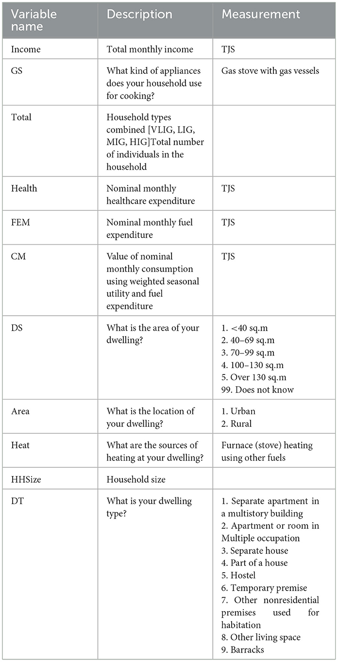
Table 2. Description of variables.

Apart from this, multiple regression analysis was completed to determine the effect of fuel expenses on healthcare expenditure.

$\begin{array}{r}Y=\text{β}0+\text{β}1X1+\text{β}2X2+\text{β}3X3+\text{β}4X4+\text{β}5X5+\text{β}6X6\\ +\text{β}7X7+\text{ ε}i\\ Health=\text{β}0+\text{β}1FEM+\text{β}2DS+\text{β}3CM+\text{β}4Area+\text{β}5Heat\\ +\text{β}6HHSize+\text{β}7DT+\text{ ε}i\end{array}$

The study used SEVs' nominal monthly healthcare expenditure (Health) as the dependent variable, with explanatory variables including nominal monthly expenditure on fuel (FEM), dwelling size (DS), the value of nominal monthly consumption using weighted seasonal utility and fuel expenditure (CM), location (Area), source of heating for the dwelling (Heat), household size (HHSize), and dwelling type (DT) (see Table 2).

Apart from multiple regression analysis, the model was examined using Ordinary Least Square methods (OLS) to estimate the parameters of the constructed model.

Empirical results

Fuel poverty

The fuel poverty level was calculated based on data regarding the fuel expenditure of HHs, utilizing the above-mentioned equations. First, equivalized disposable income was derived by calculating the ratio of the disposable income of HHs to the number of household members. The next step in evaluating energy poverty involved the extraction of equivalized fuel cost by dividing nominal monthly fuel expenditure by the number of household members. The proportion of the two calculated ratios indicated the fuel poverty level. The total percentage of fuel-poor households was found to be 30.3% out of 2,808 HHs, with an average fuel poverty level of 17.7% (see Table 3).

Table 3

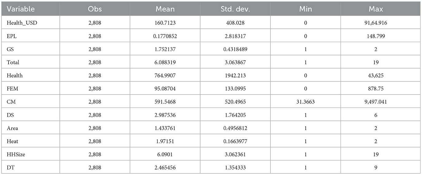
Table 3. Descriptive statistics of variables.

This implies that a minority of observed households live in fuel poverty. Nevertheless, according to Hills (2011), families with low-income experience higher levels of energy poverty, which could be obscured by high-income families. Thus, considering each income group separately is essential to observe the true extent of fuel poverty. The level of energy poverty in VLIG was nearly 46%, on average. This percentage indicates that VLIG households spent almost half of their monthly income on fuel and faced severe energy poverty. Families in LIG experienced a much lower fuel poverty rate than in the first group, with a mean value of 11%. This figure still indicates an extreme level of energy poverty; hence, LIG is also considered to be living in fuel-poor conditions. The level of energy poverty in MIG, on the other hand, showed minimal results, averaging 6%. Finally, HIG families experienced a negligible 3% of fuel poverty, on average. The last two groups are above the fuel poverty level and, therefore, are not classified as energy poor. Based on the findings, it can be stated that families with high and middle incomes masked the true evaluation of fuel poverty levels, as more vulnerable individuals were from very low and low-income households (see Table 4).

Table 4

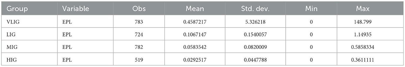
Table 4. Descriptive statistics of variable (EPL) by thresholds.

Correlation analysis of fuel requirement

Correlation analysis is a tool that measures the degree of linear association between two variables, where the correlation coefficient (“r”) illustrates the strength of the linear relationship. The experimental variable is considered to be stochastic, which has a probability distribution, while the independent variable has fixed values in repeated sampling (Gujarati and Porter, 2009).

Pearson's correlation matrix was conducted between the following variables: nominal monthly healthcare expenditure (Health_USD), which was converted from TJS to USD, fuel poverty level (EPL), and appliances used by households for cooking (GS). The findings show a low positive correlation between Health_USD and EPL (r = 0.0264), and GS and EPL (r = 0.0055), across all 2,808 households. The GS, in turn, is negatively correlated with Health_USD (r = −0.0267). The results indicate that the observed variables are not highly correlated with each other (see Table 5).

Table 5

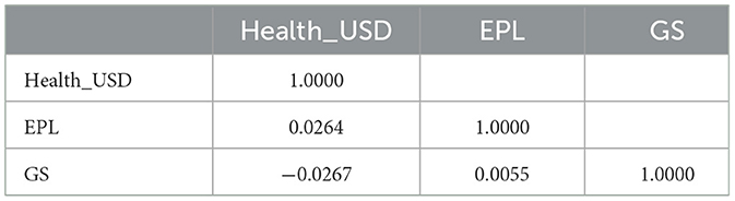
Table 5. Correlation between variables.

Consideration of correlation analysis in each income threshold detected a positive correlation between EPL and Health_USD (r = 0.0898), and GS and EPL (r = 0.0065), while a negative correlation was found between GS and Health_USD (r = −0.0727), in VLIG. Overall, it is evident that all variables in VLIG are not significantly correlated, as the correlation coefficients are low. The next group's assessment (LIG) illustrated the correlation of EPL and Health_USD, and GS and Health_USD to be similar to those in the previous group (r = 0.0608 and r = −0.0329). The correlation matrix, however, showed a negative relationship between GS and EPL, which is considerably higher than in VLIG (r = 0.1839). The correlation analysis in MIG revealed typical low correlations between variables for this study. A relatively higher, but negative, correlation in MIG was observed between GS and EPL (r = −0.2171). In the HIG, the correlation between GS and Health_USD differed from the other groups' outcomes, indicating a positive correlation (r = 0.0139). The remaining variables are correlated similarly to the previous groups' results, showing no strong correlation (see Table 6).

Table 6

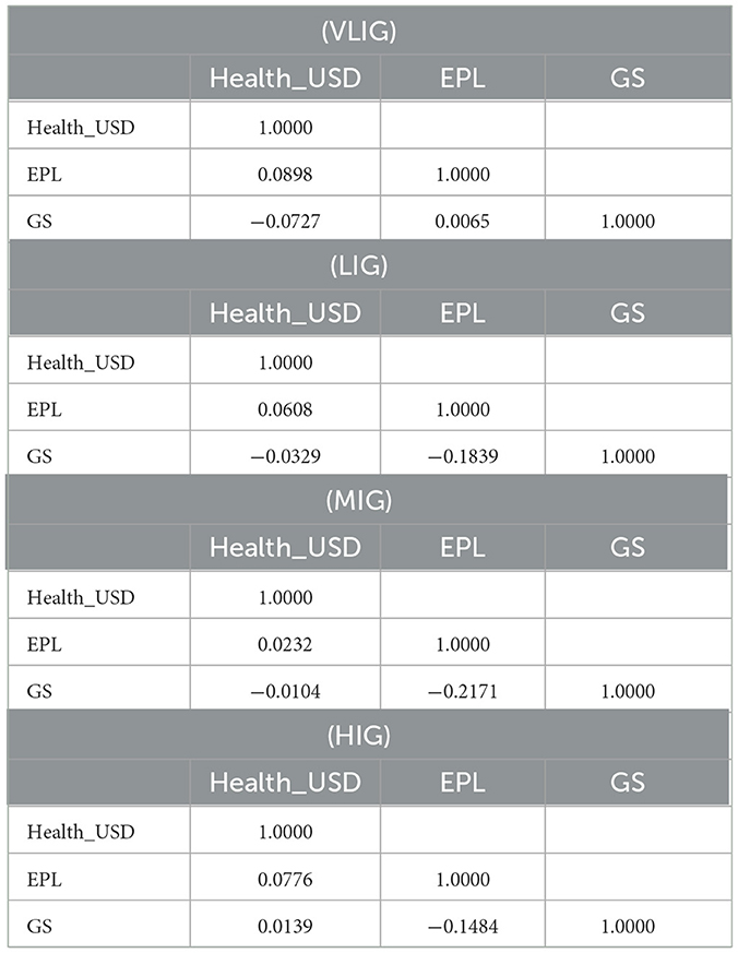
Table 6. Correlation between variables by thresholds.

In addition, the correlation matrix found a very low positive correlation between the residual (u) and the variables (EPL, GS). This indicates that the observed variables are exogenous (see Table 7).

Table 7

Table 7. Correlation between error term and SEVs.

Regression analysis of fuel poverty model

Regression analysis was performed to investigate the influence of energy poverty on healthcare expenditure. The regression outcomes revealed no significant relationship between energy poverty and healthcare expenses when considering all households (2,808 HHs), including four income groups: VLIG, LIG, MIG, and HIG. This implies that EPL is statistically insignificant at a 95% confidence interval. Thus, an increase in fuel poverty does not affect the amount of expenditure on healthcare (see Table 8). Nevertheless, to draw a proper conclusion on the influence of energy poverty on health-related expenses, each income group was examined.

Table 8

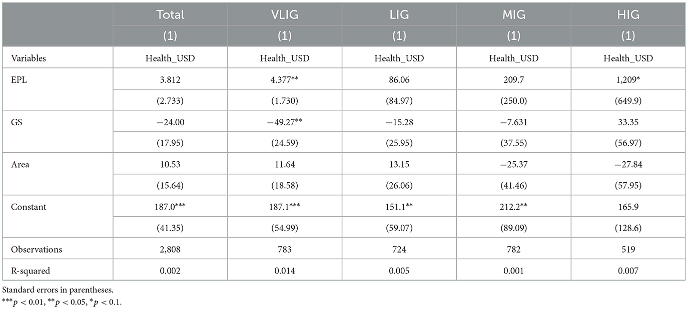
Table 8. Regression analysis of fuel poverty.

Regression results demonstrate a significant relationship between fuel poverty and healthcare expenditure at a 95% confidence interval. This suggests that a one percent increase in energy poverty leads to a $4.38 increment in healthcare expenses. The current effect might indicate that families living in fuel-poor conditions spend almost half of their budget on energy requirements. Hence, households from VLIG consume fewer high-quality goods and more low-quality goods, which could reflect health-oriented problems that require certain expenses. The use of gas stoves with gas vessels for cooking was found to negatively impact healthcare expenditure. Being statistically significant at p < 0.05, the GS negatively affects the expenses on health, where a one-unit increase in the use of gas stoves results in a 49.27 dollars decrease in healthcare expenditure. This impact may illustrate that the use of a gas stove for cooking is safer in terms of health-oriented consequences than other fuel resources. However, the area is statistically insignificant at a 95% confidence interval. Hence, regardless of location, people with very low incomes suffer from energy poverty (see Table 8).

The remaining three groups were also observed, but the findings indicated that all results were statistically insignificant and had no influence on healthcare expenditure. The VLIG was found to be the most vulnerable among all groups.

Correlation analysis between healthcare expenditure and SEVs

Pearson's correlation matrix was conducted among the following variables: nominal monthly fuel expenditure (FEM), consumption of seasonal utility (CM), dwelling size (DS), location of housing (Area), type of heating appliance (Heating), number of household members (HHSize), and dwelling type (DT).

Households in total (2,808)

The correlation between FEM and Health across all households is very low, with r = 0.06 being positive. FEM's correlation with CM is also positive and low (r = 0.17) for total households, whereas CM correlates positively with Health with a score of 0.84. DS correlates positively with Health, FEM, and CM as well, with very low scores of r = 0.004, 0.15, and 0.08 respectively. Area correlates positively with Health, FEM, CM, and DS, with most of correlations being very low and only the one between Area and FEM being higher (r = 0.55). The correlation between Heat and majority of the variables is negative and low, with the only positive correlation being between Heat and Health with a coefficient of 0.007, which is still quite low. The HH size correlates positively with majority of the variables, including Health, FEM, CM, DS, and Area, with the correlation between HH size and FEM and HH size and CM being above r = 0.30. The only negative correlation for HH size is with Heat, which is r = −0.05, also low. DT's most significant correlation is with Area, with 0.32 being a positive correlation; the rest are a combination of negative and positive correlations, which are of low significance.

Households from VLIG (783)

The correlation between Health and FEM for the VLIG is positive and low, with r = 0.07, whereas the correlation between CM and health is positive and one of the highest across groups, with r = 0.83. CM and FEM's correlation is positive but much lower than the previous one (r = 0.25) for the same type of households. DS correlates positively with Health, FEM, and CM, but with low scores below 0.2. Area's correlations with FEM appear to be significant with a coefficient of 0.55, while other variables correlate positively with Area at a very low level, below 0.2 at most. Heat is only positively correlated with Health, with a very low number. The rest of the correlations for Heat are negative and not very significant, with most scores ranging from r = −0.10 to −0.28. The household size correlates positively with every variable mentioned before, with the highest level of correlation being with FEM (r = 0.39). HH size was found to be negatively correlated with Heat, with a very low level of correlation. DT correlates positively with most variables, except for HH size and healthcare expenditure. Every correlation for DT is of low coefficient level, with the highest being under 0.30 (correlation with area) (see Table 9).

Table 9

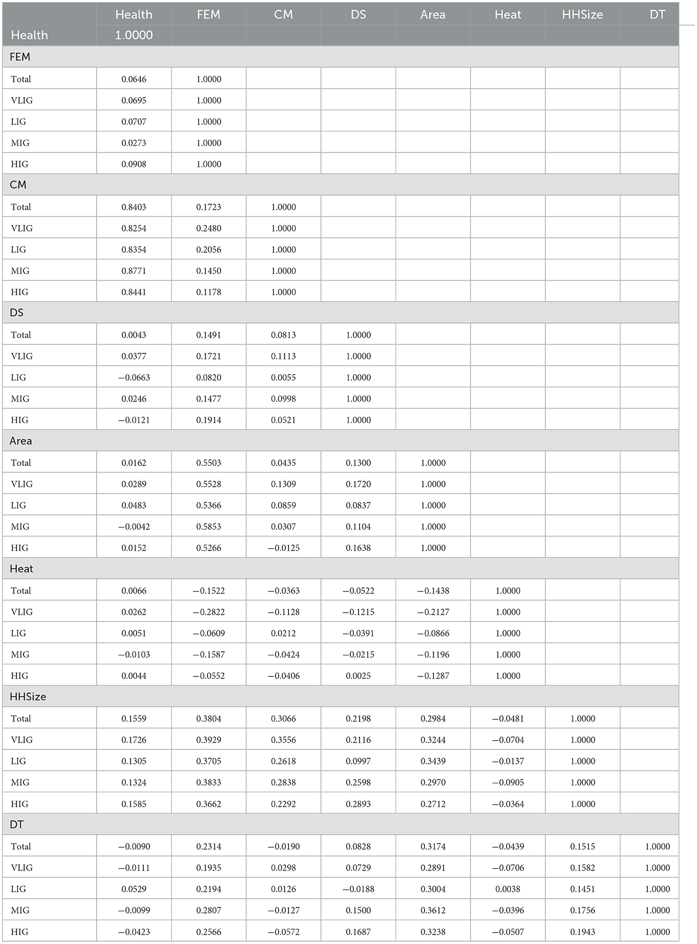
Table 9. Correlation analysis of healthcare expenditure and SEVs.

Households from LIG (724)

The correlation between health expenditure and fuel expense is low and positive, with r = 0.07 for the LIG. Within the same income level, the correlation between CM and health is significant, yielding r = 0.84, making it one of the most significant correlations in the research. In the same group, CM's correlation with health is much lower, forming r = 0.20. DS correlates negatively with health, while FEM and CM correlate positively, but with very low levels of significance below 0.1. The area's correlations with the stated variables are positive, with the only significant one being the one with FEM (r = 0.54). Heat shows no significant correlations with any of the variables and presents a combination of positive and negative correlations, with the positive ones being those with Health and CM. HHSize correlates positively with every previously mentioned variable, with its most significant correlation coefficients of 0.37 and 0.34 with FEM and Area, respectively. Its only negative correlation is with Heat, which is not significant for the research. DT correlates positively with most of the variables, with its most significant correlation being the one with Area (r = 0.3). The rest of the variables correlate at very low levels, including the only negative correlation with DS (see Table 9).

Households from MIG (782)

Within MIG, the correlation between healthcare expenditure and fuel expenditure is very low, reaching a positive coefficient of 0.03. The most notable correlation here is between CM and Health, with r = 0.88, whereas CM's correlation coefficient with FEM is 0.15. DS correlates positively with the previously mentioned variables, but all correlations are of low significance. Area's correlations indicate that the most significant one is with FEM (r = 0.59). It is worth noting that the only negative correlation for Area is with health, and it is at a low level of significance. In turn, Heat correlates negatively with every variable, and the numeric values for each of them are low in terms of significance for the research. HHSize in MIG correlates positively with majority of variables, with the numeric values of “r” ranging from 0.13 to 0.38, where the highest is with FEM. The only negative correlation here is between HHSize and Heat, which is still below the point of significance. DT's correlations consist of combinations again, with positive correlations observed between DT and FEM, DS, Area, and HHSize, where the correlation with Area at r = 0.36 is the highest. The rest of the scores appear to be below the significance point (see Table 9).

Households from HIG (519)

Among HIG, FEM does not correlate significantly with Health. Interestingly, CM also correlates positively with health in this group, with an “r” of 0.84, whereas its correlation with FEM is low. DS correlates positively with FEM and CM, although those correlations are of low significance. Health correlates negatively with DS, but the level of correlation remains very low. For Area, the most significant correlation is with FEM, yielding r = 0.53, which is positive. The rest of the correlations for Area are of low significance, with the one with CM being the only negative one. Heat, in turn, correlates positively with health and DS; every correlation with Heat is of low significance for the research. HHSize correlates negatively with Heat, while the rest of the correlations are positive, with the one with FEM being relatively stronger at r = 0.37. DT's correlations again show a combination of positive and negative, with most being very low in significance. The only higher ones are the correlations between DT and FEM and DT and Area, at r = 0.26 and 0.32, respectively (see Table 9).

Regression analysis of healthcare expenditure and SEVs

The study observed the influence of nominal monthly fuel expenditure on nominal monthly healthcare expenditure. To check the significance of the effect, OLS multiple regression analysis was conducted.

Households in total (2,808)

Regression analysis on the overall data of 2,808 HHs demonstrated that the model is appropriate, due to the significant result in F-statistics at a 95% confidence interval. The adjusted R² value was 0.725, which implies that exogenous variables explain the stochastic variable for 72.5%. The model for the total number of households is estimated as follows:

$\begin{array}{r}\text{Health}=-1,609--1.074\text{FEM}--47.11\text{DS}+3.303\text{CM}+184.1\\ \text{Area}+336.3\text{Heat}--60.31\text{HHSize}+41.83\text{DT}+\text{ εi}\\ {(0.182)}^{***}{(11.24)}^{***}{(0.0392)}^{***}{(48.42)}^{***}{(117.5)}^{***}\\ {(7.228)}^{***}{(15.09)}^{***}\end{array}$

The current model specifies that the nominal monthly fuel expenditure of the total number of households (2,808 HHs) significantly influences the nominal monthly health expenditure at p < 0.05. Each TJS increase in fuel expenditure reflects in a 0.18 TJS decrease in health expenditure. Such a negative relationship might be explained through consumption perspectives. High expenses on fuel represent larger consumption of energy resources, which may lead to health deterioration. Family budgets, on the other hand, may suffer from high contributions to fuel requirements, which may cause constrained expenditure on health, as people may consume cheaper, health-oriented goods of lower quality. The amount of monthly consumption of seasonal utility (CM) is statistically significant and has a positive effect on health expenditure. For every increment in consumption of seasonal utility, there is an increase of 3.3 TJS in healthcare expenditure. The size of the dwelling (DS) negatively affects the expenditure on health, showing a statistically significant result. Each square meter increase of the dwelling size reduces health expenditure by 47.11 TJS.

The justification for certain effects is that the wider a dwelling, the more space is available for habitation. Hence, energy consumption escalates, which leads to higher spending on fuel. This certainly shrinks the budget allocated to other expenses, including health-related aspects. Being statistically significant, the location of households' habitation (Area) positively influences healthcare expenditure. Families living in urban areas spend more on health issues than those households living in rural areas. The type of heating (Heating) was also found to affect health expenditure, with significant t-statistics. HHs that heat their dwellings with furnaces using fuels, except for coal, are likely to experience higher health expenses. Household size (HHs) was found to negatively influence healthcare expenditure, showing a statistically significant figure. An increase in household size by one family member decreases health expenditure by 60.31 TJS. Such an effect is irrefutable, as a larger number of people requires higher fuel consumption. This shrinks income per family member; consequently, expenses on health narrow down. Findings suggest that dwelling type positively contributes to healthcare expenditure, indicating significant probability (see Table 10).

Table 10

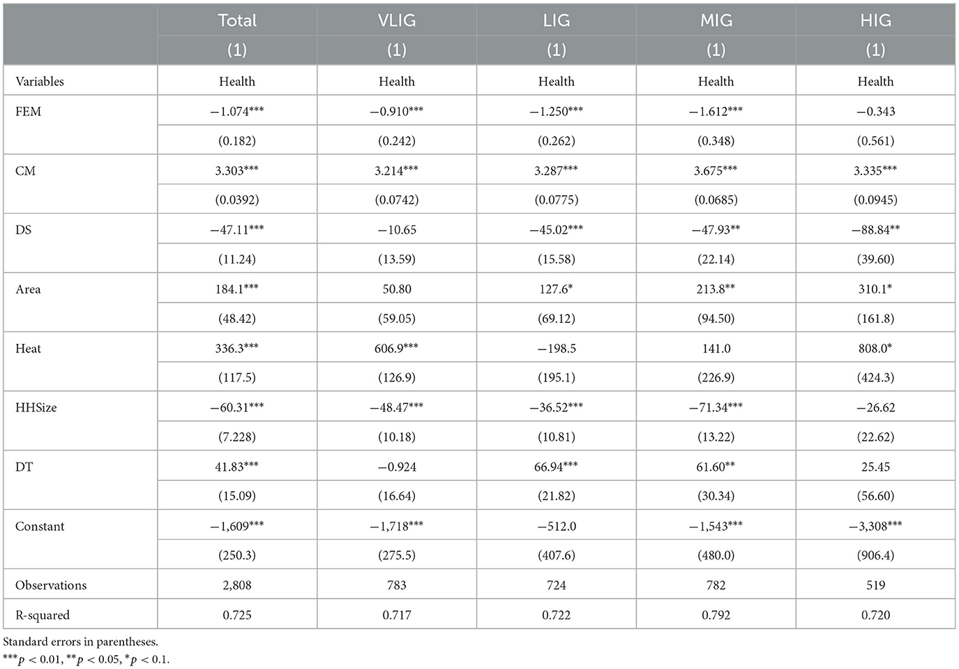
Table 10. Regression analysis by thresholds.

Households from VLIG (783)

Regression results on VLIG households yield an adjusted R² of 0.717, suggesting that the applied independent variables describe the dependent variable for 71.7%. The model is accurate as its F statistic shows significance at a 95% confidence interval. The built model is specified as follows:

$\begin{array}{r}\text{Health}=-1,718--0.910\text{FEM}--10.65\text{DS}+3.214\text{CM}\\ +50.80\text{Area}+606.9\text{Heat}--48.47\text{HHSize}-0.924\text{DT}+\text{ εi}\\ {(0.242)}^{***}{(13.59)}^{***}(0.0742)(59.05){(126.9)}^{***}{(10.18)}^{***}(16.64)\end{array}$

From the equation, it is evident that fuel expenditure (FEM) negatively affects healthcare expenditure, as each increment in fuel expenditure results in a 0.9 TJS decrease in health expenses. Price and budget perspectives may explain the current effect. An increase in energy prices reduces the purchasing power of VLIG households by diminishing the amount available for spending on health. The VLIG is the most vulnerable among all other income groups in terms of budget constraints, hence even a negligible increase in energy expenses results in a reduction of expenditure on other sectors, including healthcare. Dwelling size (DS) was also found to be statistically significant, with a negative relationship toward healthcare expenditure. Every square meter increase in dwelling size leads to almost an 11 TJS reduction in spending on health. Consumption of utility (CM), dwelling type (DT), and location of housing (Area) are found to be statistically insignificant, thus they do not affect the stochastic variable. The heating appliance used (Heating), as well as household size (HHSize), showed positive and negative significant influences, respectively (see Table 10).

Households from LIG (724)

The findings from multiple regression analysis on LIG households yield an adjusted R² of 0.722, indicating that the chosen exogenous variables depict the experimental variable for 72.2%. The F-statistic illustrates significant results at p < 0.05. The estimated model is provided below:

$\begin{array}{r}\text{Health}=-512--1.250\text{FEM}--45.02\text{DS}+3.287\text{CM}\\ +127.6\text{Area}--198.5\text{Heat}--36.52\text{HHSize}+66.94\text{DT}+\text{ εi}\\ {(0.262)}^{***}{(15.58)}^{***}{(0.0775)}^{***}{(69.12)}^{*}(195.1){(10.81)}^{***}{(21.82)}^{***}\end{array}$

The model presents statistically significant outcomes regarding the impact of fuel expenditure (FEM) on health expenditure (Health), which revealed a negative relationship. Each TJS increase in fuel expenditure correlates with a 1.3 TJS decrease in healthcare expenditure. Variables such as dwelling size (DS), dwelling type (DT), utility consumption (CM), and household size (HHSize) are found to be highly significant. The effects, however, differ in terms of signs. Dwelling size and household size negatively impact health expenditure, while the other variables positively influence health-related spending (see Table 10).

Households from MIG (782)

Results of multiple regression analysis on MIG households show an adjusted R² of 0.792. This indicates that the examined independent variables strongly describe the dependent variable for 79.2%. The model is properly specified as its F-statistic is significant at a 95% confidence interval. The formulated model is presented as follows:

$\begin{array}{r}\text{Health}=-1,543--1.612\text{FEM}--47.93\text{DS}+3.675\text{CM}\\ +213.8\text{Area}+141.0\text{Heat}--71.34\text{HHSize}+61.60\text{DT}+\text{ εi}\\ {(0.348)}^{***}{(22.14)}^{***}{(0.0685)}^{**}{(94.50)}^{**}(226.9){(13.22)}^{***}{(30.34)}^{**}\end{array}$

Every increment in fuel expense (FEM) decreases expenditure on healthcare (Health) by more than 1.6 TJS. The expense of fuel is price dependent, as higher prices for energy resources lead to larger fuel expenditures. Thus, family income restricts the purchasing power of MIG households, which challenges food and non-food consumption, including the health sector. Dwelling size (DS) was found to be highly significant in MIG, as each square meter increase is associated with a 47.93 TJS decline in healthcare expenditure. The interpretation of such an influence combines several factors, one of which is the budget effect. Larger housing increases the demand for energy use, which takes up a larger proportion of the family budget. This constrains the purchasing power of MIG households, thus shrinking the available capital for healthcare spending. Consumption of utility (CM), on the other hand, positively affects health-related expenditure, where for every TJS increase in monthly consumption, there is almost a 3.7 TJS growth in healthcare expenditure. Utility consumption is driven by demand; thus, an increase in demand for utility leads to higher healthcare expenses. The area has a lower but still significant influence on health spending. Heating appliances (Heating) are shown to be statistically significant, as the use of furnaces with fuels, excluding coal and electricity, raises spending on health by 141 TJS. Heating with fuel resources such as gas may lower fuel expenditure due to relatively cheaper prices. This increases the purchasing power of individuals, which raises demand for further consumption, and consequently boosts expenditure on healthcare. Household size (HHSize) has a negative significance in MIG. Each additional family member decreases the household's purchasing power, leading to a 71 TJS decline in healthcare expenditure (see Table 10).

Households from HIG (519)

Regression outcomes on HIG households yield an adjusted R² of 0.720, clearly showing that observed variables strongly describe the examining variable for 72%. The following model was properly specified, as its F-statistic is significant at p < 0.05:

$\begin{array}{r}\text{Health}=-3,308--0.343\text{FEM}--88.84\text{DS}+3.335\text{CM}\\ +310.1\text{Area}+808.0\text{Heat}--26.62\text{HHSize}+25.45\text{DT}+\text{ εi}\\ (0.561){(0.0945)}^{***}{(39.60)}^{**}{(161.8)}^{*}{(424.3)}^{*}(22.62)(56.60)\end{array}$

Unlike other income groups, HIG households' healthcare expenses are found to be not influenced by their monthly fuel expenditure. This situation can be explained from an income perspective. HIG households' fuel expenditure covers a negligible proportion of their budget, due to the relatively high income available for consumption. Nevertheless, dwelling size is observed to be statistically significant and has a negative relationship with healthcare expenditure. Every additional square meter of dwelling is associated with almost an 89 TJS increase in spending on health. This implies that no matter which income layer the household belongs to, dwelling size significantly reduces healthcare expenditure. Consumption of utility (CM), the use of heating appliances (Heating), and location of dwelling (Area) are found to be of lower significance. The dwelling type, on the other hand, was revealed not to influence healthcare expenditure in HIG (see Table 10).

The existing factors that may cause observed effects of SEVs on households' healthcare expenditure will be covered in the conclusion part.

Application of ordinary least squares (OLS) model

The model was also tested against OLS assumptions, where the problem of heteroscedasticity occurred. To tackle the problem of heteroscedasticity, the Huber–White robust standard errors method was applied (see Table 11). Robust regression provides an alternative to OLS regression with less stringent assumptions. Namely, the regression coefficient estimates improve despite the existence of possible outliers that violate the OLS assumption of normally distributed residuals. The use of the Skewness–Kurtosis test demonstrated that residuals are not normally distributed in the regression model. The reason for certain violations of assumption is the existence of peaks in data that skew the distribution to the right. Nonetheless, the data contains a large number of observations, which mitigates the problem of normality. The Linktest produced significant outcomes, indicating that the regression model is correctly specified. The correlation matrix was utilized to discover the relationship between residuals and exogenous variables, where results showed that there is no correlation between the observed variable and the error term. This provides evidence that there is no endogeneity problem. Furthermore, the variance inflation test (VIF) was conducted, where, based on the rule of thumb, no perfect multicollinearity was found.

Table 11

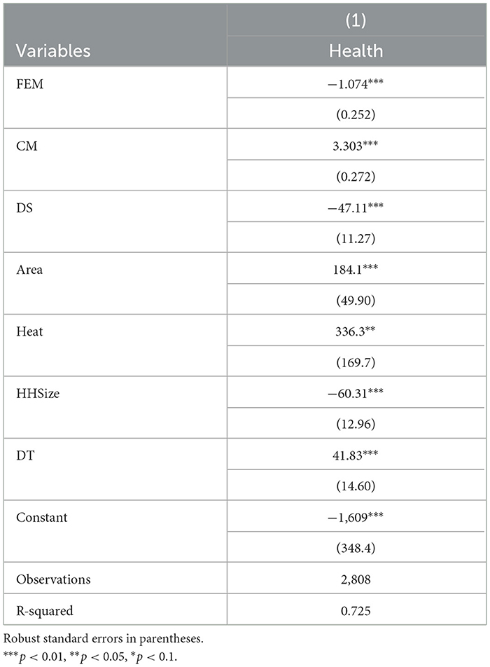
Table 11. Regression analysis, robust.

Conclusion

Limited access to energy resources, wealth gaps, the sustainability crisis, and more—these elements magnify the concept of fuel poverty, which comes along with increased medical bills. This empirical analysis was carried out to evaluate the influence of different socio-economic variables (SEVs) on the healthcare expenditure of households in Tajikistan. The research applied secondary data on 2,808 households, covering a diverse number of SEVs. The data was categorized by HHs' monthly income and formed four groups—specifically, very low-, low-, middle-, and high-income classes. The current study examined fuel poverty based on the consumption expenditure approach and demonstrated that over 30% of observed households (2,808 HHs) live in energy-poor conditions, on average. Separate consideration of each income category revealed that families with high incomes faced a mere 3% of the energy poverty level, on average. Similarly, MIG households experienced a slightly higher level of fuel poverty (6%) than the previously mentioned group. These two income classes were considered to be beyond the energy poverty line. The low-income group was identified to be in fuel poverty with an 11% rate. Not surprisingly, the very low-income group has undergone grave energy poverty, where almost half of families live in fuel poverty. Similar to Sharma's study, it was concluded that very-low-income households are the most vulnerable and affected by energy poverty among all other income groups. From Hills' perspective on energy poverty, families with relatively high fuel costs and low incomes incur additional spending to heat their dwellings during winter, unlike those households from higher social strata. These extra costs are beyond their control, leading to an opportunity cost of indoor dwelling temperature for other necessary goods. This exacerbates the challenges that households living in poverty experience. Facing severe fuel poverty results in habitation at relatively low temperatures during the heating season, which contributes to an increased number of deaths. It can be concluded that energy poverty is a grave issue that negatively affects health conditions by cutting down the proportion of the budget available for healthcare services. The basic belief regarding health enhancement is that it is driven by a high-income level, as it allows for the procurement of health services. The findings in this research align with Pickett and Wilkinson (2015), who observed a tight relationship between imbalanced public income and healthcare expenditure burden. Nevertheless, some research has found the absence of causality between personal income and healthcare expenditure. The majority of those studies explain such an argument through the consequences of inaccurate measurement of income scales and constrained periods of observation. The World Health Organization (2014) notes that in developing countries, such as Tajikistan, public resources are inadequately dispensed in a framework of health services that should correspond to the necessities of people in poverty. Reallocation of the public budget, as well as the application of debt-relief capital, could potentially increase government spending on healthcare services. Empirical results presented in this paper provide evidence of the existing effect of fuel expenditure on healthcare spending. This conclusion overlaps with Owoundi's findings on the relationship between fuel requirement spending and healthcare expenditure. Owoundi evaluated the strong influence of fuel costs on individual health expenditure, justifying certain outcomes by the extensive spending of the family budget on fuel needs. In addition, it is notable that his work highlighted the low-income class as being more affected by an increase in fuel costs, as it raises pressure on the households' budget and opportunity costs for other necessities. The results demonstrate how people facing greater health needs attribute very low priority to spending related to health. This contradicts previous suggestions claiming that physically challenged individuals are likelier to be sicker and that such households' spending on healthcare is higher. This information differs from findings in research on developed countries. The user fees that were established to cope with governmental budget constraints were not intended to bring negative results for health spending and discourage people from seeking healthcare. A cost-sharing policy in the area must provide some safety net for those who cannot afford healthcare for economic reasons. This way, the most disadvantaged individuals who need it the most are not excluded from accessing healthcare. The Nouna District developed a community-based health insurance program after conducting studies. It is expected to be an effective tool for the efficient use of resources and financial protection for low-income populations (in low-income countries), with less effective institutional capacity that cannot accommodate risk-pooling strategies across the nation, and informal sectors are one of the main work providers for majority of the population. In the area where the study was conducted, individuals with the lowest income faced “catastrophic” health spending. The estimations from this paper regarding the influence of heating on healthcare were supported by results in the background literature. For instance, in one of the reviewed studies, it was found that mortality rates during winter decrease with a reduction in heating prices. The natural gas prices for electricity decreased by 42% from 2005 to 2010; if we consider the estimate of the elasticity of mortality from various causes concerning the heating price, the results show that the decrease in heating prices brought a 1.6% reduction in mortality during winter among households that use natural gas as their primary heating source. There was also a 0.9% decrease in the mortality rate in winter in the USA when natural gas prices decreased, which is significant because 58% of American households were found to be using natural gas to heat their homes. This trend resulted in a 0.4% decrease in annual mortality, which is equivalent to 11,000 fatal cases a year.

It can be concluded that this impact is so significant on a large scale that it should be taken into account for evaluating the net health impact of natural gas shale production. The study highlights the advantages and benefits of policies to decrease energy costs for households, with a special focus on low-income groups. The study illustrates the energy poverty level of randomly selected households from different social strata in Tajikistan. Representatives from each income group were observed separately as well. Conducted research found the impact of fuel poverty on healthcare expenditure only in the very low-income class. The regression model was controlled by two variables: the type of appliances used by the households for cooking, namely the use of a gas stove, and the location of the dwelling. The control variables were chosen in accordance with background literature on the measurement of fuel poverty, though it was impossible to build a stronger model due to data limitations. Nonetheless, the results would be more precise if more instruments controlled the exogenous variables. Apart from this, expenditure perspectives on fuel and healthcare were analyzed to estimate the potential influence of fuel expenditure on health spending. The effect was found to be negative but statistically significant. The model used seven control variables that were selected based on literature review, all of which were found to have a significant impact on healthcare expenditure. This empirical model is accurate, although the use of appropriate instrumental variables would improve it further.

It was not possible to study the impact of fuel poverty on households' health expenditure based on age groups within the framework of this research. This is a limitation of the current investigation. The impact of fuel poverty on health expenditure among different age groups remains an avenue for future research.

Data availability statement

The original contributions presented in the study are included in the article/supplementary material, further inquiries can be directed to the corresponding author.

Ethics statement

Ethical approval was not required for the study involving human participants in accordance with the local legislation and institutional requirements. Written informed consent to participate in this study was not required from the participants in accordance with the national legislation and the institutional requirements.

Author contributions

ST: Data curation, Formal analysis, Investigation, Methodology, Software, Writing – original draft, Writing – review & editing. OK: Conceptualization, Data curation, Methodology, Supervision, Validation, Writing – review & editing. BE: Conceptualization, Data curation, Methodology, Project administration, Supervision, Writing – original draft, Writing – review & editing. AM: Writing – review & editing, Methodology, Project administration, Validation, Investigation.

Funding

The author(s) declare that no financial support was received for the research and/or publication of this article.

Conflict of interest

The authors declare that the research was conducted in the absence of any commercial or financial relationships that could be construed as a potential conflict of interest.

Publisher's note

All claims expressed in this article are solely those of the authors and do not necessarily represent those of their affiliated organizations, or those of the publisher, the editors and the reviewers. Any product that may be evaluated in this article, or claim that may be made by its manufacturer, is not guaranteed or endorsed by the publisher.

References

Baker, W. (2001). “Fuel poverty and ill health,” in Centre for Sustainable Energy. Available online at: https://www.cse.org.uk/downloads/reports-and-publications/fuel-poverty/fuel-poverty-ill-health.pdf (accessed 21 March, 2024).

Google Scholar

Banerjee, S. G., Barnes, D., Singh, B., Mayer, K., and Samad, H. (2015). Power for All: Electricity Access Challenge in India. Banerjee, Washington, DC: World Bank. Available online at: http://documents.worldbank.org/curated/en/562191468041399641/pdf/922230PUB0978100Box385358B00PUBLIC0.pdf (accessed March 21, 2024).

Google Scholar

Boardman, B. (1991). Fuel Poverty: From Cold Homes to Affordable Warmth. Available online at: https://books.google.com/books/about/Fuel_Poverty.html?id=HwYtAAAAMAAJ (Accessed March 21, 2025).

PubMed Abstract | Google Scholar

Bouzarovski, S. (2014). Energy poverty in the European Union: landscapes of vulnerability. Wiley Interdiscipl. Rev. Energy Environ. 3, 276–289. doi: 10.1002/wene.89

PubMed Abstract | Crossref Full Text | Google Scholar

Davillas, A., Burlinson, A., and Liu, H. H. (2023). Getting warmer: fuel poverty, objective and subjective health and well-being. Energy Econ. 106:105794. doi: 10.1016/j.eneco.2021.105794

Crossref Full Text | Google Scholar

Du, H., and Zhang, B. (2025). Revisiting the energy-happiness paradox in China: the role of housing outcomes. J. Happiness Stud. 26:20. doi: 10.1007/s10902-025-00860-0

Crossref Full Text | Google Scholar

FxRates (2020). Convert 2013 Tajikistani Somoni to US Dollar using Latest Foreign Currency Exchange Rates. Available online at: https://www.fxrateslive.com/TJS/USD/2013 (accessed March 21, 2024).

Google Scholar

Gujarati, D., and Porter, D. (2009). Basic Econometrics (5th ed). New York, USA: Douglas Reiner.

Google Scholar

Hills, J. (2011). “Fuel poverty: the problem and its measurement,” in Interim Report of the Fuel Poverty Review. Available online at: http://sticerd.lse.ac.uk/dps/case/cr/CASEreport69.pdf (accessed March 21, 2024).

Google Scholar

Hills, J. (2012). “Getting the measure of fuel poverty,” in Final Report of the Fuel Poverty Review. Available online at: http://sticerd.lse.ac.uk/dps/case/cr/CASEreport72.pdf (accessed 21 March 2024).

Google Scholar

International Labor Organization (2020). Eastern Europe and Central Asia. Available online at: https://www.ilo.org/moscow/news/WCMS_429145/lang–en/index.htm (accessed March 21, 2024).

Google Scholar

Kahouli, S. (2020). An economic approach to the study of the relationship between housing hazards and health: The case of residential fuel poverty in France. Energy Econ. 85:104592. doi: 10.1016/j.eneco.2019.104592

Crossref Full Text | Google Scholar

Kanagawa, M., and Nakata, T. (2018). Socio-Economic Impacts of Energy Poverty Alleviation in Rural Areas of Developing Countries. Available online at: https://www.researchgate.net/profile/Toshihiko_Nakata2/publication/278684170_Socioeconomic_impacts_of_energy_poverty_alleviation_in_rural_areas_of_developing_countries/links/5583c9d008ae4738295b8e6e/-Socioeconomic-impacts-of-energy-povertyalleviation-in-rural-areas-of-developing-countries.pdf (accessed March 21, 2024).

Google Scholar

Kanti, A. (2017). 1.3 Million Deaths Every Year in India Due To Indoor Air Pollution. New Delhi: Bwbusinessworld. Available online at: http://businessworld.in/article/1-3-Million-DeathsEvery-Year-In-India-Due-To-IndoorAirPollution/09-09-2017-125739/ (accessed March 21, 2024).

Google Scholar

Owoundi, J. (2013). “The weight of health expenditure on household income in Cameroon,” in Ministry of Economy, Planning and Regional Development. Available online at: https://www.researchgate.net/publication/290826910_The_Weight_of_Health_Expenditures_on_Household_Income_in_Cameroon/link/59e3a314aca2724cbfe3ae8c/download (accessed March 21, 2024).

Google Scholar

Pan, L., Biru, A., and Lettu, S. (2020). Energy poverty and public health: global evidence. Energy Econ. 101:105423. doi: 10.1016/j.eneco.2021.105423

Crossref Full Text | Google Scholar

Pickett, K., and Wilkinson, R. G. (2015). Income inequality and health: a causal review. Soc. Sci. Med. 128, 316–326. doi: 10.1016/j.socscimed.2014.12.031

PubMed Abstract | Crossref Full Text | Google Scholar

Raghavan, S. (2018). Power losses: technology to the rescue. Hindu. Available online at: https://www.thehindu.com/todays-paper/tp-business/powerlosses-technology-to-therescue/article17669369.ecen

Google Scholar

Ranjan, R., and Singh, S. (2017). Energy Deprivation of Indian Households: Evidence from NSSO Data. MPRA Paper 83566.

Google Scholar

Sharma, S. (2019). Socio-economic determinants of energy poverty amongst Indian households: a case study of Mumbai. Energy Policy 132, 1184–1190. doi: 10.1016/j.enpol.2019.06.068

Crossref Full Text | Google Scholar

Ucal, M., and Günay, S. (2022). Household happiness and fuel poverty: a cross-sectional analysis on Turkey. Appl. Res. Qual. Life 17, 391–420. doi: 10.1007/s11482-020-09894-3

Crossref Full Text | Google Scholar

UNDESA (2014). A Report on Electricity and Education: The Benefits, Barriers, and Recommendations for Achieving the Electrification of Primary and Secondary Schools. Available online at: https://sustainabledevelopment.un.org/index.php?page=viewandtype=400andnr=1608andmenu=1515 (accessed March 21, 2024).

Google Scholar

United Nations (2019). Goal 17: Sustainable Development Knowledge Platform. Available online at: https://sustainabledevelopment.un.org/sdg17 (accessed March 21, 2024).

Google Scholar

World Bank (2017). “Jobs, skills, and migration survey 2013,” in Microdata Library. Available online at: https://microdata.worldbank.org/index.php/catalog/2813/datafile/F31 (accessed March 21, 2024).

Google Scholar

World Health Organization (2014). World Health Statistics. Geneva: World Health Organization. Available online at: https://www.who.int/gho/publications/world_health_statistics/2014/en/ (accessed March 21, 2024).

Google Scholar