Comparison of multi-coil and multi-frequency frequency domain electromagnetic induction instruments

Introduction: Characterization of the shallow subsurface in mountain catchments is important for understanding hydrological processes and soil formation. The depth to the soil/bedrock interface (e.g., the upper ~5 m) is of particular interest. Frequency domain electromagnetic induction (FDEM) methods are well suited for high productivity characterization for this target as they have short acquisition times and do not require direct coupling with the ground. Although traditionally used for revealing lateral electrical conductivity (EC) patterns, e.g., to produce maps of salinity or water content, FDEM inversion is increasingly used to produce depth-specific models of EC. These quantitative models can be used to inform several depth-specific properties relevant to hydrological modeling (e.g. depths to interfaces and soil water content).

Material and methods: There are a number of commercial FDEM instruments available; this work compares a multi-coil device (i.e., a single-frequency device with multiple receiver coils) and a multi-frequency device (i.e., a single receiver device with multiple frequencies) using the open-source software EMagPy. Firstly, the performance of both devices is assessed using synthetic modeling. Secondly, the analysis is applied to field data from an alpine catchment.

Results: Both instruments retrieved a similar EC model in the synthetic and field cases. However, the multi-frequency instrument displayed shallower sensitivity patterns when operated above electrically conductive grounds (i.e., 150 mS/m) and therefore had a lower depth of investigation. From synthetic modeling, it also appears that the model convergence for the multi-frequency instrument is more sensitive to noise than the multi-coil instrument.

Conclusion: Despite these limitations, the multi-frequency instrument is smaller and more portable; consequently, it is easier to deploy in mountainous catchments.

1 Introduction

Characterization of the near subsurface at high spatial and temporal resolutions is a key task for many areas of critical zone research. Typically, such quantification is done with intrusive sampling and subsequent laboratory analyses. However, this can be prohibitively expensive and time-consuming. In addition, such work may not be technically feasible, for instance, if the field site is remote or the soils are impenetrable. Alternatively, geophysical tools offer an attractive approach as they can provide information about the geophysical properties of the subsurface. Frequency domain electromagnetic (FDEM) methods are sensitive to electrical conductivity (EC), which is correlated with several hydrologically important parameters, e.g., water content (1), clay content (2), and salinity (3).

FDEM devices were first developed in the 1970s and were initially used for salinity mapping (e.g., 3). Since then, their use has been expanded to map information about soil texture (e.g., 4), water content (e.g., 5), organic matter (e.g., 6), and soil thickness (7). Unlike electrical resistivity tomography (ERT) methods (e.g., 8, 9), which are also sensitive to subsurface EC, FDEM methods do not require direct contact with the ground, making it an attractive tool for wide-scale coverage. FDEM instruments typically consist of one transmitter (Tx) coil and one, or more receiver (Rx) coils aligned on a rigid boom, see Figure 1A. The Tx coil produces a primary oscillating electromagnetic field at a given operating frequency, which induces eddy currents in the subsurface (Figure 1). The strength of these eddy currents is proportional to the subsurface EC. These eddy currents generate a secondary electromagnetic field which is detected by the Rx coil. The imaginary component of the complex ratio, HS/HP is related to the EC of the subsurface.

Figure 1

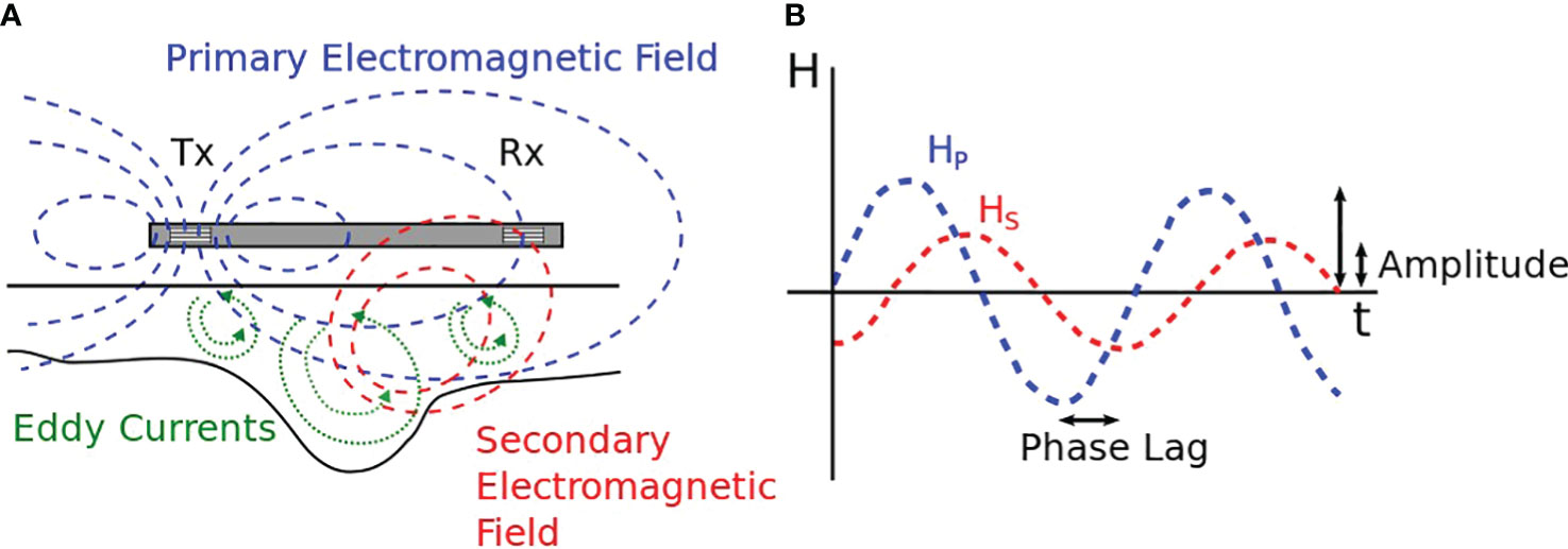
Figure 1 Internal working of an FDEM instrument. (A) shows the transmitter coil (Tx) emitting a primary transient electromagnetic field (Hp). (B) Given the amplitude ratio (HS/HP) and the phase shift between the primary and secondary fields, knowledge about the electrical properties of the subsurface can be inferred. Reproduced from McLachlan et al. (20).

Larger separation distances between the Rx and the Tx coils have larger (and deeper) investigation volumes. Similarly, lower operating frequencies of the primary electromagnetic field result in deeper investigation depths. The investigation volume also depends on the orientation (e.g., horizontal or vertical) of Tx and Rx coils, and the electrical conductivity of the subsurface. We redirect the reader to McNeill (10), Doolittle and Brevik (11) and Altdorff et al. (12) for more in depth explanation of the FDEM technique. For ground-based environmental applications with relatively low EC (i.e., < 100 mS/m), the Rx-Tx separation distance is generally considered to be more important for dictating the depth of investigation than differing operating frequencies. Nonetheless, several authors have noted the ability of multi-frequency FDEM measurements to reveal vertical variability in EC (e.g, 13, 14, and 15). Consequently, there is interest in assessing the ability of both instruments.

For environmental applications, the imaginary component of the HS/HP ratio is commonly expressed as an apparent electrical conductivity (ECa) (e.g., 1, 2, and 4). These values are termed “apparent” because they refer to the theoretical homogenous subsurface with an equivalent imaginary component. However, when the subsurface is heterogenous, measurements with different sensitivity patterns will obtain a different ECa for the same location. The in-phase component of the HS/HP ratio is related to magnetic susceptibility. This value is not as commonly used in environmental studies, but it has been used in archaeological studies with both multi-coil and multi-frequency instruments (e.g., 16, 17); and also in agricultural sites with high soil metal contents (e.g., 18). This work focuses on the quadrature component of FDEM measurements, and focuses on EC values usually encountered in environmental applications (i.e., 15 to 150 mS/m) for synthetic modeling.

Many applications of FDEM have utilized relationships between specific soil parameters and ECa (see review by 19). Although these relationships can characterize spatial variability, they generally do not consider vertical variability. Moreover, in many cases, these relationships can be highly site-specific. Alternatively, there has been interest in developing quantitative EC models from FDEM data. By utilizing several measurements with differing sensitivity patterns, distributions of EC can be modeled using inverse methods (e.g., 13–15, 20). Many instruments have been designed to provide information about different depths (volumes) of the subsurface simultaneously. The sensitivity of FDEM measurements depends upon subsurface EC and device properties, i.e., the separation distance and orientation of coils, the operating frequency, and the height of the instrument above the ground. For instance, the multi-Rx Explorer system (GF Instruments, Brno, Czechia) has intercoil spacings of 1.48, 2.82, and 4.49 m. In comparison, the multi-frequency GEM-2 system (Geophex) collects data at multiple frequencies, ranging from 425 Hz to 92.775 kHz.

Instrument performance for a given application can be assessed by conducting synthetic modeling to assess differences in sensitivity and impacts of measurement noise. It is also worthwhile to make practical comparisons of such multi-frequency and multi-coil devices. For instance, multi-frequency devices are more lightweight and consequently are well suited in remote terrains. Furthermore, their lightweight nature makes them well suited for mounting in uncrewed aerial vehicles (UAVs), e.g., Bjerg et al. (21).

This work compares the GF Instruments Explorer and the Geophex GEM-2 devices in an alpine catchment. It should be noted that Altdorff et al. (12) undertook similar work previously, where they compared multi-coil and multi-frequency instruments to assess the correlation between ECa with cation exchange capacity, water content, and silt content. Similarly, Doolittle et al. (22) also compared apparent values of both types of instrument for salinity appraisal. However, the novelty of the work is that the focus is on translating raw FDEM data into electrical conductivity models. Indeed, we do not convert ECa to soil properties of interest but rather investigate the fundamental differences in the inversion results between the two types of instruments with a synthetic and field case. We use the open-source inversion software EMagPy (20) to process the field data and generate synthetic models.

2 Materials and methods

2.1 Instruments

In this study, we compare the GF Instruments Explorer and the Geophex GEM-2. The Explorer is a multi-coil instrument with one Tx and three Rx coils; in comparison, the GEM-2 operates at six frequencies and contains a single Tx-Rx pair and an additional “bucking coil”. Whilst the Explorer records primary and secondary fields in the Rx coil, the Rx coil of the GEM-2 only records the secondary field and the influence of the primary field on the Rx coil is removed by the bucking coil (23). Given that the primary field is stronger than the secondary field, the purpose of the bucking coil in the GEM-2 is to increase the accuracy of measuring the secondary field in the Rx coil. Nonetheless, in both cases the derived HP/HS can be expressed as an ECa value. Both instruments can be oriented in vertical coplanar (VCP) or horizontal coplanar (HCP) orientations. During a survey, one of the two coil orientations can be used. Consequently, three Explorer and six GEM-2 measurements can be recorded simultaneously. One would have to traverse the survey area twice to collect all possible coil configurations. However, this is often impractical, especially for mapping large areas. Hence, only one configuration (e.g., the HCP configuration with the deepest sensitivity) is used in this work.

The Explorer operates at a constant frequency of 10 kHz. The larger the distance between the transmitter and the receiver, the deeper the depth of investigation, see Figure 2. The GEM-2 has a single Tx-Rx pair with a fixed distance of 1.66 m and an additional “bucking coil” at 1.035 m from the Tx coil. The GEM-2 is able to operate at multiple frequencies between 425 Hz and 92.775 kHz. As noted, for multi-frequency instruments, higher frequency measurements are associated with shallower depths of investigation, see Figure 2. Table 1 summarizes the coil configurations available and their nomenclature in EMagPy (20).

Figure 2

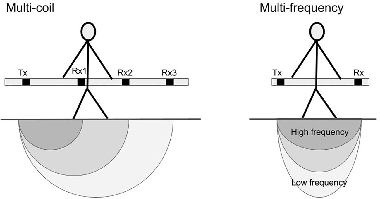
Figure 2 Schematic representation of the investigation volume Modified from Altdorff et al. (12) and Keiswetter and Won (24). Multi-coil instruments operate at a single frequency and investigate deeper using larger separation between transmitter (Tx) and receiver (Rx) coils. Multi-frequency instruments have a single Tx-Rx pair and utilize different frequencies to vary the depth of investigation.

Table 1

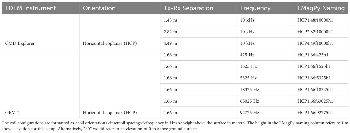
Table 1 Coil configuration of the Explorer and GEM-2 instruments.

2.2 Synthetic study

The synthetic study compares the instruments using a three-layer model with two EC values (10 and 150 mS/m) (Figure 3). These values were chosen as they are representative of the geology of the site. The left half of the model (samples 1 to 10) presents a conductor with an increasing thickness on top of a resistor, and the right half (samples 11 to 20), presents a resistor on top of a conductor. The forward model response of this model was generated using EMagPy for the coil configurations of each instrument, as specified in Table 1. The forward model used was the “Full-Solution with Low Induction Number” (FSlin) model. This model computes the HS/HP ratio using Maxwell’s equation (25) and converts the quadrature values into ECa values using the low induction number (LIN) approximation (see 26). In EMagPy, it is referred to as the “full solution” as opposed to the simplified “cumulative sensitivity” model of McNeill (10).

Figure 3

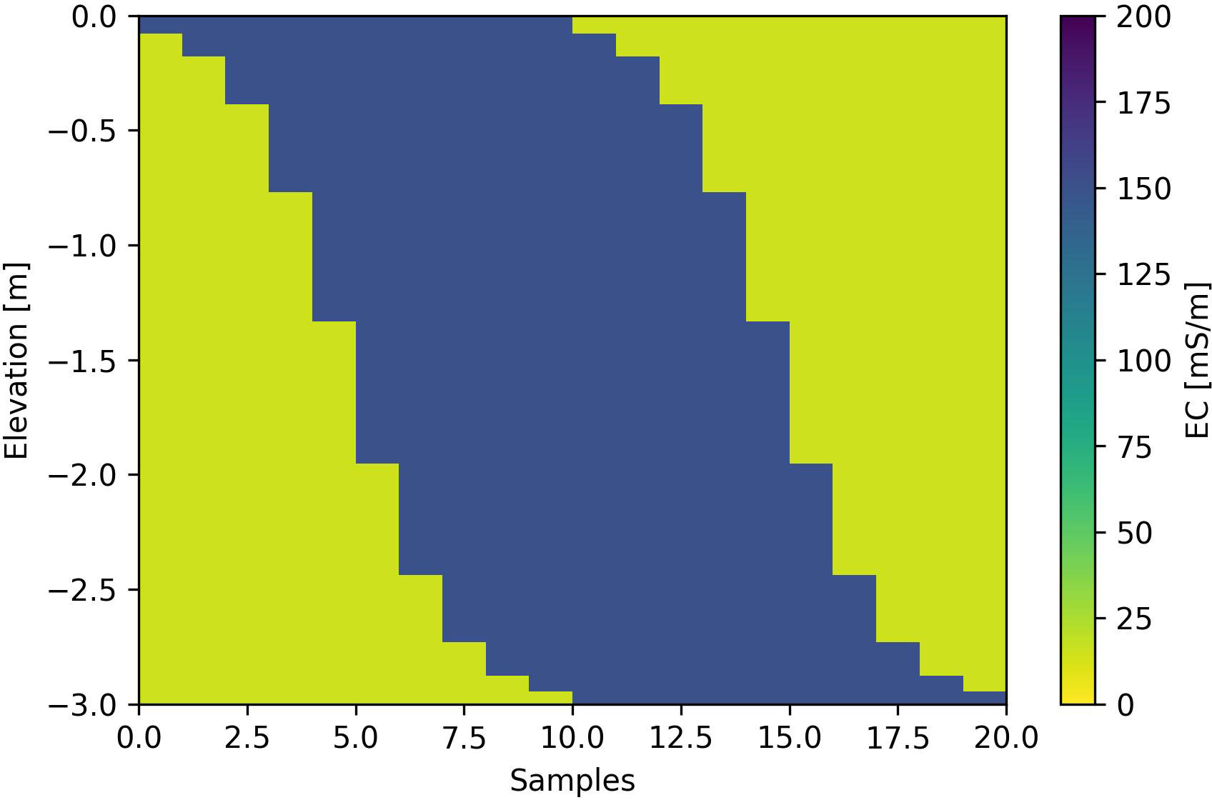
Figure 3 Synthetic three-layer model with two contrasting electrical conductivities of 15 and 150 mS/m.

It should be noted that the LIN approximation assumes that the subsurface EC is not “too high”, i.e., McNeill (10) notes discrepancies above 100 mS/m. Despite these limitations, commercial instruments often use the LIN approximation as it provides a conversion from the HS/HP ratio to the more intelligible ECa quantity, which uses the same units as EC. This linear conversion, utilized in the FSlin model, is applied for data generated for both instrument configurations.

The synthetic data were inverted to assess the ability of both instruments to resolve the model specified in Figure 3. The data were corrupted with 1, 2, 5, and 10% Gaussian noise to simulate the typical error levels encountered in field data. However, it should be noted that in field conditions, the error levels are likely to be different between coils. For instance, lower frequencies of GEM-2 measurements typically have higher errors, as do shorter Tx-Rx separation distances. The strategy chosen here uses the robust parameter estimation solver ROPE (27) implemented in the spotpy Python package (28). This solver generates several parameter sets (in this case, two depths and three-layer EC values) and tries to find the optimum set. We used the standard error from the top 10% best realizations to obtain an error on the estimated parameters.

For the synthetic case, no vertical smoothing was applied. Similarly, each sample of the conductivity model is independent (i.e., no lateral smoothing), meaning that each model only considers 1D depth variations. In order to compare both instruments, individual 1D inversions using the ROPE optimization algorithm are done.

2.3 Field data

The field data were acquired with both instruments in an alpine catchment in Alento (Salerno, Italy). The Alento field site is part of the Italian network of Critical Zone Observatories; the site is instrumented with numerous permanent sensors (e.g., weather stations, capacitance sensors, tensiometers, and cosmic-ray neutron probes; see Nasta et al. (29) for more information). The sub-catchment (MFC2), near the village of Monteforte Cilento, is where the data for this work was collected. MFC2 has a typical agroforestry landscape with olive trees, and cherry orchards used for wood production. The sub-catchment is formed by a regolith layer on top of an argillaceous turbidite bedrock (30). The sub-catchment covers an area of approximately 250 m x 250 m (Figure 4). The FDEM data was collected for both sensors in October 2020 (not on the same day). Both sensors were carried by the operator above the ground at 1 m elevation. The acquisition lasted about 1h and common points were acquired during the survey to check for temperature drift. The drift was found to be negligible.

Figure 4

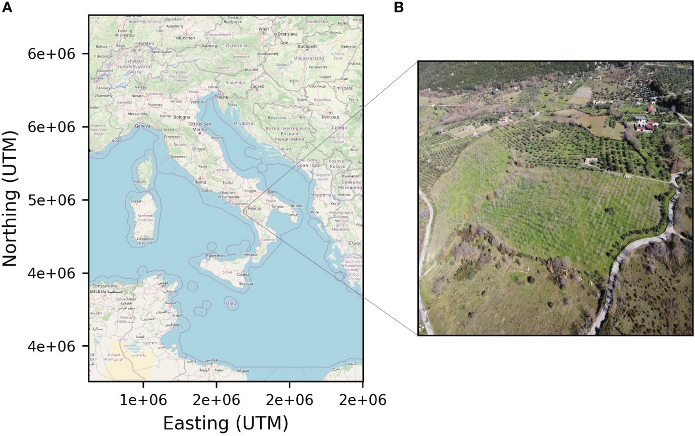
Figure 4 (A) Location of the catchment in Italy and (B) Aerial view of the catchment area of the MCF 2 site. Background map from OpenStreeMap, reproduced under Open Data Commons Open Database License (ODbL).

The field data are inverted using a 1D model with fixed depths and vertical smoothing (no lateral smoothing) using the Gauss-Newton solver. The same depths and smoothing parameters were chosen for both instruments.

3 Results

3.1 Synthetic modeling

3.1.1 Sensitivity analysis

Figure 5 shows the local normalized sensitivity profiles of the HCP coil configurations for both instruments over homogeneous 15 and 150 mS/m subsurfaces at 1 m height. The different coil specifications have different sensitivity profiles; hence they contain information about different depth-specific properties. For the higher EC for the multi-frequency instrument (Figure 5D), it can be seen that the sensitivity functions are shifted upwards with respect to the lower EC values. This shift is particularly evident for the two highest frequencies, 63.025 and 92.775 kHz. This process can be attributed to the more conductive body concentrating the signal closer to the instrument. This effect seems more pronounced for the multi-frequency than the multi-coil instrument.

Figure 5

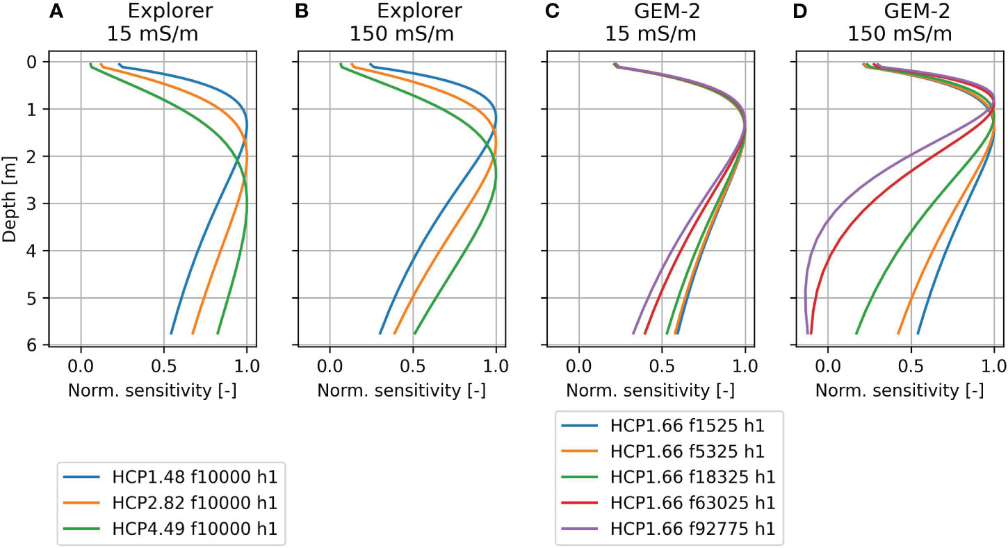
Figure 5 Normalized sensitivity profiles of the Explorer (A, B) and the GEM-2 (C, D) over a homogeneous 15 mS/m (A, C) and 150 mS/m (B, D) subsurface. Different lines represent different coil configurations of the instruments.

Importantly, it can be seen that for the low EC subsurface, there is a substantial overlap in sensitivities for the GEM-2 measurements, particularly in comparison to the multi-coil instrument. This overlap indicates that for low electrical conductivity environments, the GEM-2 system will struggle to resolve vertical variability in electrical conductivity.

3.1.2 Inversion of synthetic data

The inversion results for the synthetic data are shown in Figure 6. Synthetic data generated for both instruments retrieved the structure in the synthetic model relatively well. The boundaries are indicated with red lines in Figure 6. For measurement samples 5 to 10, where high conductivity values dominate the conductivity model, the depth of the resistor is underestimated compared to the true model for both instruments. This effect seems to be greater for the GEM2 model. Without prior knowledge, such a situation would lead to an erroneous interpretation of the subsurface. On the other hand, the model recovered from the GEM-2 instrument seems to be better at delineating the boundary between the layers for samples 12 to 20, i.e., a resistor on top of a conductor. This better delineation can most likely be attributed to the larger number of coil configurations. Indeed, in this case, the GEM-2 provides 6 data points (coil configurations) vs 3 for the Explorer to fit a model with 3 parameters (2 conductivities and 1 depth).

Figure 6

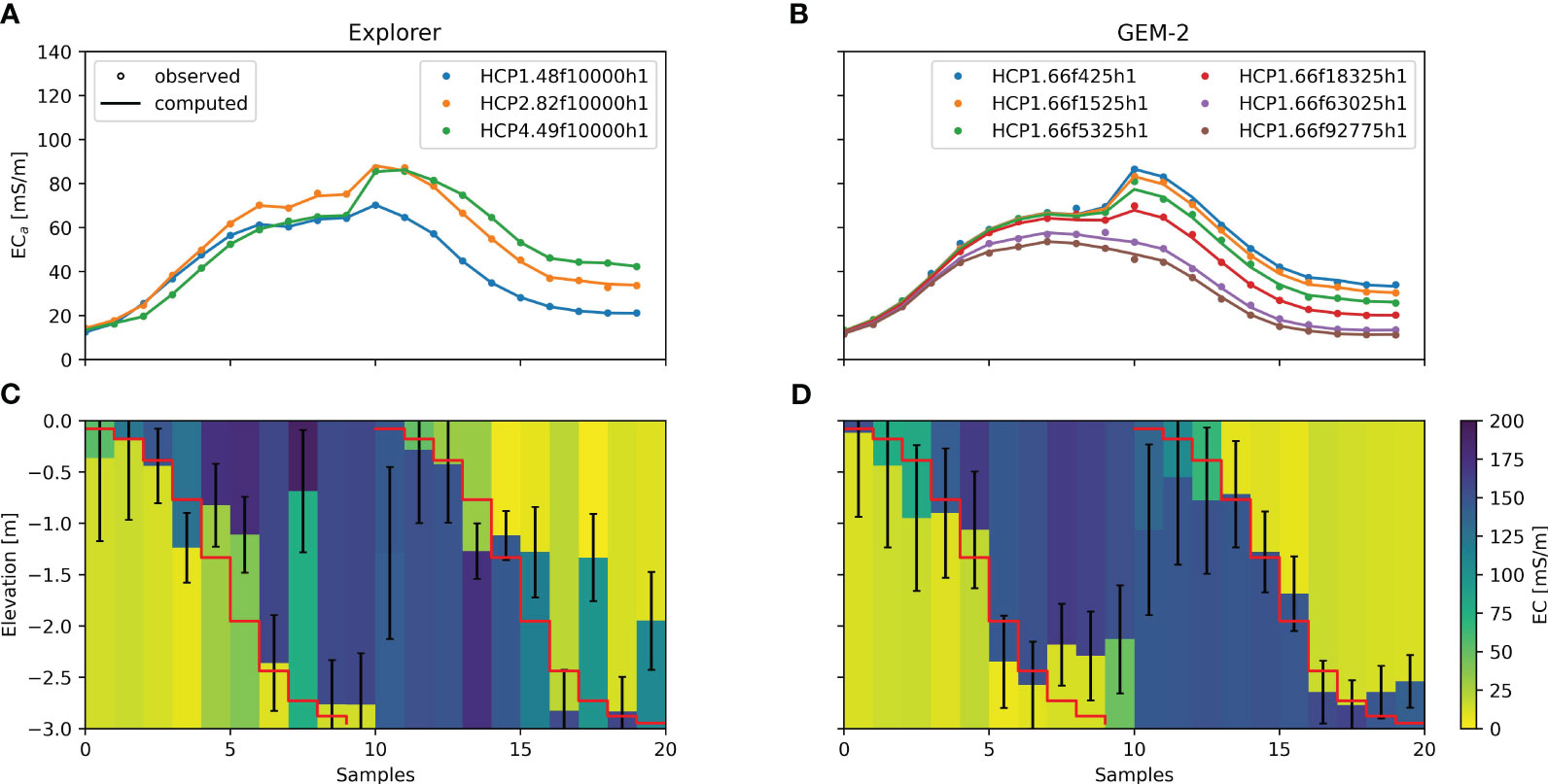
Figure 6 Inversion results from a two-layer model with low EC (15 mS/m) and high EC (150 mS/m) values and 2% Gaussian noise (e.g., Figure 3). (A, B) Observed apparent electrical conductivity and the one computed after inversion. (C, D) Recovered structure after inversion (ROPE solver, L1 regularization). The red lines represent the true boundaries between the layers of 15 and 150 mS/m layers. The error bars represent the standard deviation of the mean based on the 10% best realizations.

3.1.3 Noise effect

In Figure 7, the effect of the noise on the recovery of the model is assessed. In real conditions, noise can have multiple sources, e.g., related to instrument electronics, external infrastructure, and motion-induced noise during surveys. For instance, if the instrument wobbles and rotates substantially during surveys motion-induced noise will be introduced. Furthermore, in rugged terrains, such as the one here, a non-flat terrain (or the instrument not being maintained horizontally) can cause an overestimation or underestimation of the ECa. For instance, if surveys are conducted parallel to steep topographic contours, and the device is not parallel to the ground surface, the 1D assumption of the subsurface will not be valid. Note that no weighting of the data by the noise level is done within EMagPy with the ROPE solver, instead the resultant model is characterized by higher RMS misfit. For both instruments, a higher noise level creates larger errors in recovering the model. These errors seem to be slightly higher for the GEM-2 than for the Explorer. Here as well, the “shielding” effect, illustrated by a smaller thickness of the first layer caused by the first high conductive layer between samples 5 and 10, is visible for both instruments.

Figure 7

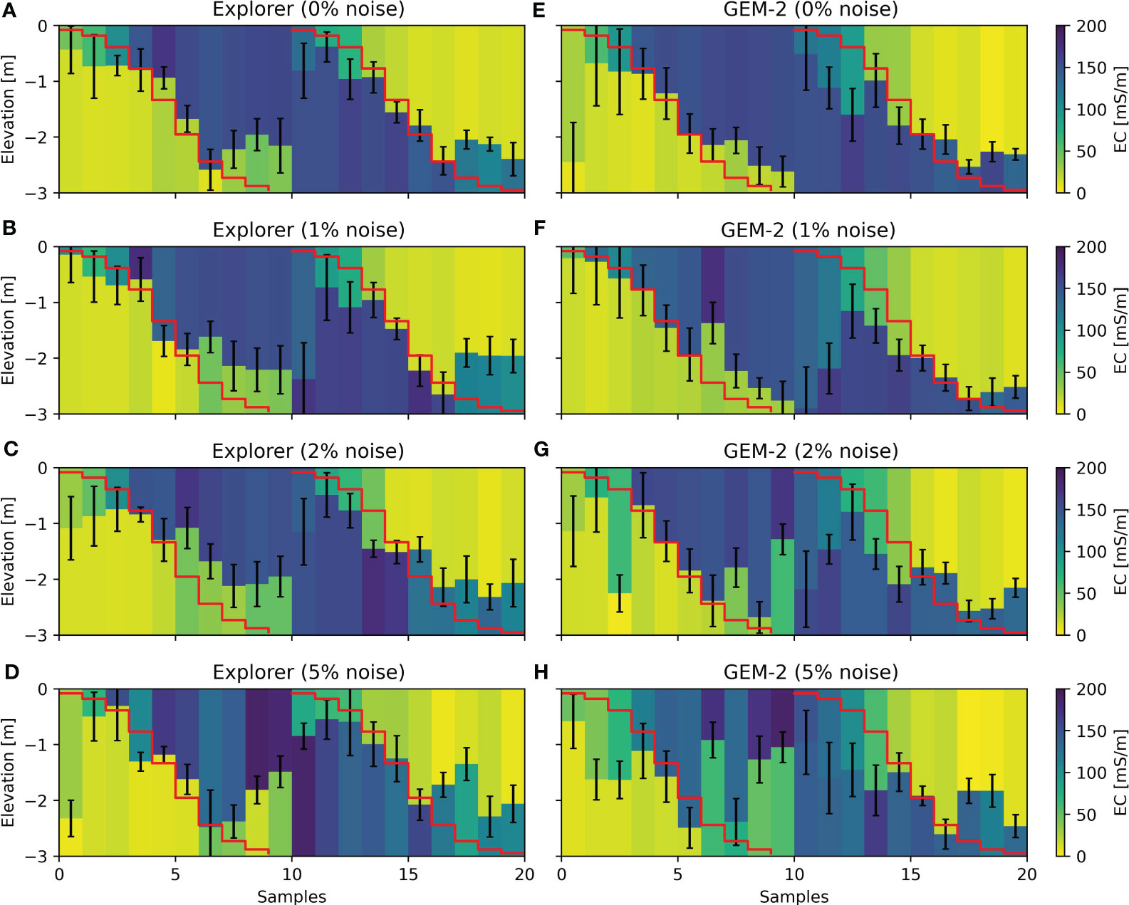
Figure 7 Effect of different noise levels (0, 1, 2, and 5% Gaussian noise) of the apparent electrical conductivity values on the inversion (ROPE solver, L1 regularization) of both Explorer (A–D) and GEM-2 (E–H) instruments. The red lines represent the true boundaries between the layers of 15 and 150 mS/m. The error bars represent the standard deviation of the mean based on the 10% best realizations. No lateral smoothing has been applied.

3.2 Field data

Figure 8 shows the measured ECa values for each operating frequency collected by the GEM-2 across the field site catchment. It can be observed that the lowest frequency (425 Hz) presents a high level of noise and is not usable. Given the deeper depth of sensitivity of lower frequency measurements, e.g., Figure 5, they should be less susceptible to surface disturbances such as height above the ground. This high level of noise does not correspond to our expectation, in this case we attribute it to instrumental failure for this specific frequency.

Figure 8

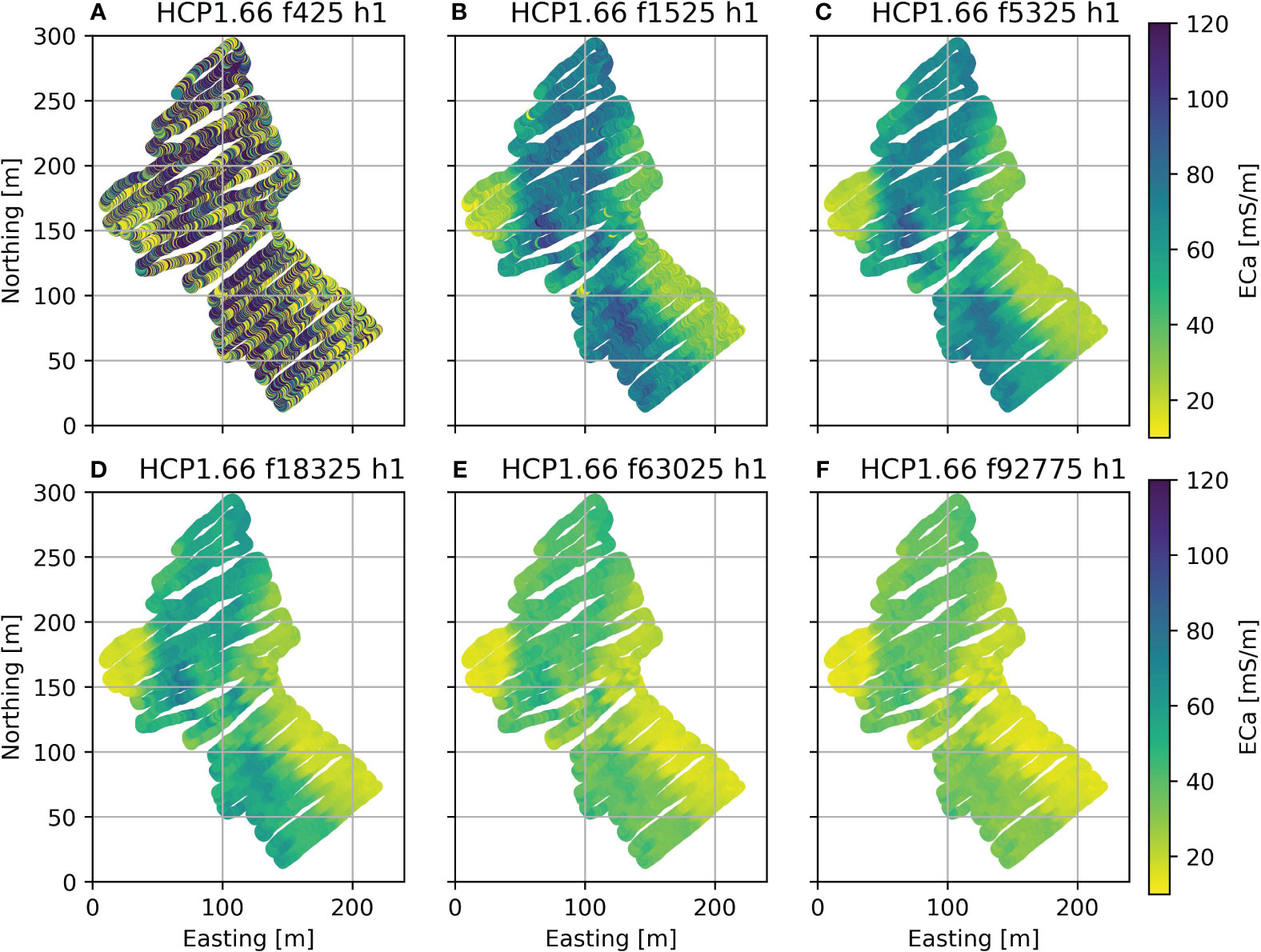
Figure 8 Measured apparent electrical conductivity (ECa) from the GEM-2 instruments. Each subplot shows a different operating frequency. Each subplot (A–F) shows a different operating frequency (425 Hz to 92775 Hz).

From Figure 8, we observed that measured ECa values range from 10 to 100 mS/m. All measurements are characterized by a conductive, 80 m wide, strip running broadly north-south. This pattern can be attributed to conductors occurring at shallower depths in the field site. It can be observed that as the frequency increases (so shallower depth of investigation), the ECa values decrease. This pattern suggests that there is a likely increase in EC with depth. For instance, these patterns agree with patterns seen in samples 12-20 of the synthetic data. The LIN approximation used also tends to underestimate the ECa for higher frequencies; but this effect alone cannot fully explain the observed pattern in this case.

Figure 9 shows the measured ECa values for each coil separation of the Explorer across the field site catchment. Although the coverage of the Explorer is less extensive than of the GEM-2, they both show the same variation, i.e. the area is more conductive in the center of the site.

Figure 9

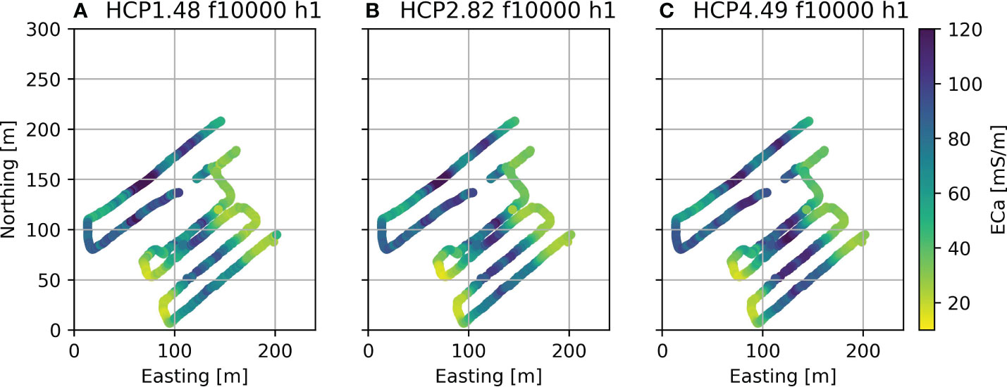
Figure 9 Measured apparent electrical conductivity (ECa) from the Explorer instruments. Each subplot (A–C) shows a different coil separation (1.48 to 4.49 m).

Based on the common locations of the GEM2 and Explorer data, the measurements were extracted and inverted (Figure 10). The same forward model (FSlin) as for the synthetic model was used but this time a greater number of layers (6 layers) with fixed, linearly increasing depths was chosen to obtain a smooth model. We choose this approach over the “variable depth” approach used in the synthetic case as we find it more suited for a field case where the structure of the subsurface is not well defined.

Figure 10

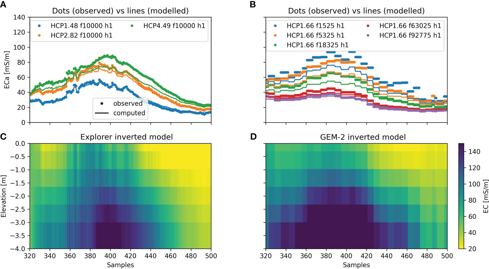
Figure 10 Observed (scatter points) and computed (plain line) apparent electrical conductivity (ECa) on common locations between Explorer (A) and GEM-2 (B) surveys. Inverted models produced are shown in (C, D).

The comparison between the observed and computed ECa (Figure 10A) shows that for the largest Explorer coil separation distance (HCP4.49 m) the computed values are underestimated, particularly for the higher ECa values. A similar feature can also be observed for the middle coil separation of the Explorer (HCP2.82 m), however the feature is less pronounced. This can be caused by a bias in the instrument calibration but ultimately affects the certainty of the final inverted model. A similar observation can be made for the GEM2 (Figure 10B) for the lower frequencies (< 63025 kHz).

From Figure 10, it can be observed that both instruments recovered the same structure with slightly different EC values. The resistive layer, 20 to 30 mS/m, is much more apparent for samples 420 and above with a depth varying from 0 to 2 m. The main differences between the two instruments are located between the samples 320 to 360. The model from the explorer data identifies a resistive layer (20 mS/m) on the shallow surface (from 0 to 1 m depth) and a fairly homogeneous layer below 60-80 mS/m. Conversely the GEM2 identifies an increasing conductivity ranging from 80 to 140 mS/m from 0 to 4 m depth.

Figure 11 shows a comparison between the inverted EC values obtained from the GEM-2 and the Explorer. Note that both models show the same range of EC and the agreement between the two instruments is linear and close to the 1:1 line. Nevertheless, on average the GEM2 instrument provides models with higher conductivity values. It should also be noted that as the conductivity increases, the difference between the resolved conductivities increases.

Figure 11

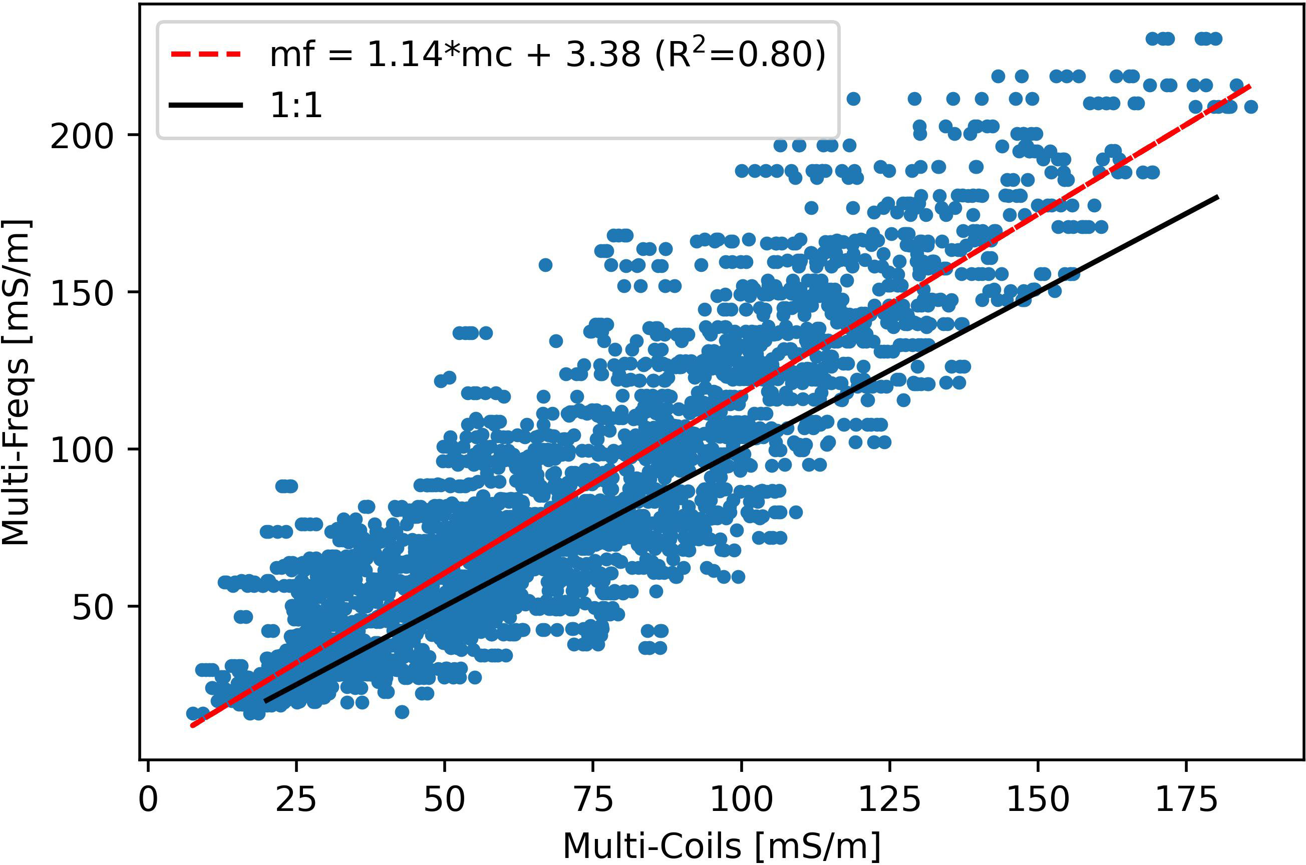
Figure 11 Comparison of inverted EC from the GEM-2 (vertical axis) and Explorer (horizontal axis) based on a common transect identified in Alento. The black line represents the 1:1 line and the red line shows a linear relationship between the inverted conductivities of both methods.

Figure 12 shows the selected inverted layer of the GEM2 dataset. It can be observed that the general pattern observed with apparent values is kept and that deeper layers show a slight increase in EC, also observed on the inverted transects shown in Figure 10D. Additionally, to the southeast of the field site, a low-conductivity anomaly can be observed, with increasing depth, the extent of this anomaly is smaller.

Figure 12

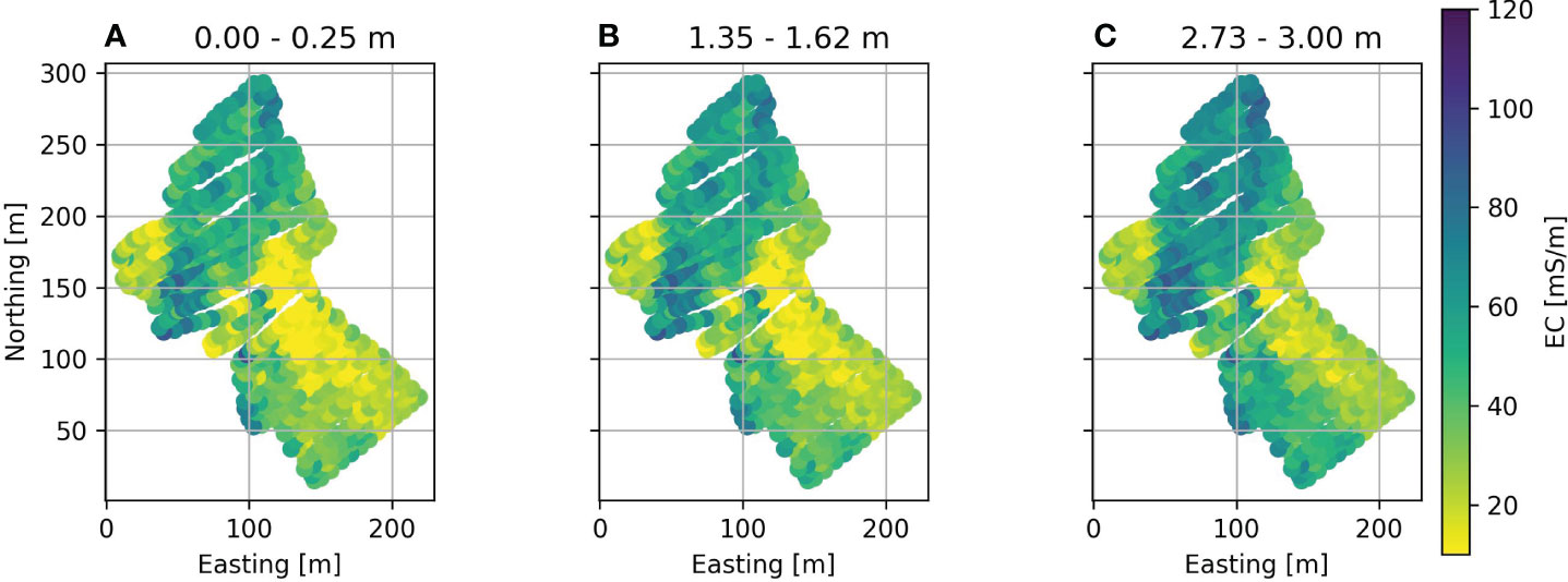
Figure 12 Inverted Inverted maps for the GEM2 dataset for different layers (A–C). The depth of the top and bottom of the layer is indicated in the subplot title.

4 Discussion

4.1 Capabilities

Both instruments have several advantages and disadvantages. The GEM2 can obtain 6 measurements simultaneously by utilizing different operating frequencies. Whereas the Explorer can collect 3 measurements simultaneously using three coil separations. Both instruments can be operated in either VCP or HCP. Consequently, additional measurements can be obtained in a second survey done in VCP mode. This second survey can improve the accuracy of the inversion, depending on the depth of the target. For a fair comparison, we limited the comparison to one orientation (HCP) for both instruments, i.e., they took a similar survey time. A comparison with both orientations can be done by modifying the notebook provided with this manuscript (see data availability section).

The sensitivity patterns of both instruments (Figure 5) are comparable over a resistive ground (15 mS/m), but a shallower sensitivity is observed for the higher frequency of the GEM2. Due to the conductive ground, most of the signal from these higher frequencies is attenuated in the shallower layer and cannot penetrate deeper, decreasing the depth of investigation. This behavior can be seen in the synthetic case, where the conductive anomaly cannot be resolved well (especially for the GEM2) between samples 8 to 10 (Figures 6, 7). In addition, the fixed Rx-Tx distance of the GEM2 leads to a smaller investigation volume than the 4.49 m Rx-Tx span of the multi-coil instrument. Another observation is that the peak of the sensitivity of the GEM2 instrument is always around the same depth (Figure 5). In contrast, the peak of the sensitivity of the Explorer shows a larger depth variation. The similar sensitivity patterns of the GEM2 measurements could indicate that there is limited value in multi-frequency instruments (as has been proposed by manufacturers of multi-coil instruments, e.g. http://www.geonics.com/pdfs/technicalnotes/tn30.pdf last consulted on 2023-09-13). However, previous work by Brosten et al. (14) demonstrated that the GEM2 was able to recover layered features of varying depths both synthetically and in the field.

4.2 Comparing the same support volume

Altdorff et al. (12) provided a comparison between multi-coil and multi-frequency instruments and used the same models as in this work (GEM2 and Explorer). Their work compared the robustness of the relationships between ECa values and soil parameters (e.g., soil moisture content). Many papers in the literature directly correlate ECa with soil parameters and neglect the support volume on which these measurements are based. Indeed, as explained, ECa readings are “apparent”. They represent a sensitivity-weighted average of the subsurface EC of the soil (weighted by the sensitivity profile of the coil configuration). Comparing an integrated value (such as ECa) with a depth-specific value (such as soil moisture at a given depth) can lead to non-robust relationships. Indeed, on more conductive ground, the sensitivity pattern of the instrument will change (Figure 5), and hence the volume investigated by the FDEM probe will vary. This observation is in agreement with Altdorff et al. (12) about the less robust relationships between ECa of multi-frequency instruments and soil properties in wet (i.e., more conductive) conditions. They found that the multi-coil devices were less impacted by this change in sensitivity patterns on the conductive ground (as shown in Figure 6). This explains why they found the relationships with the multi-coil instruments more robust in both wet and dry conditions.

While we stress that the apparent values obtained from a FDEM instrument are integrated and not depth-specific measurements, we acknowledge that inverting the information from different coil configuration to obtain a smooth depth-specific EC profiles has also disadvantages. The regularization (smoothing) used to solve the inverse problem introduces another level of uncertainty. However, it is the most appropriate way to compare field data from both instruments (Figure 10). As the same inversion settings were used for both instruments, we can reasonably assume that the same level of smoothing was introduced for both.

The comparison of the inverted EC values of both instruments for the field case (Figure 10) shows that the multi-frequency instruments resulted in EC on average 1.2 times higher than the ones from the multi-coil instruments with a small offset of 1 mS/m. The offset should not be considered here as FDEM instruments tend to provide “relative” values and need to be calibrated against other methods (e.g., ERT; see 31, 36) to provide absolute EC values. However, we expect the slope to be close to 1. From Figure 11, we can see that the points tend away from 1:1 line above 100 mS/m and become non-linear. This can be partly explained by the fact that the CMD Explorer is calibrated linearly between 50 and 100 mS/m. While the GEM-2 provides quadrature values that are then converted to ECa using the low induction number approximation. This can lead the Explorer to underestimate ECa values outside the calibration range.

Electrical conductivity is often converted to soil properties (e.g. moisture content or clay content). These properties are depth-specific and hence a direct comparison with ECa values, while often observed in the literature, can be misleading as the support volume of the ECa does not match the depth-specific soil measurement. There are two principal ways of establishing a relationship between conductivity values and soil properties. The first one involves inverting the ECa values into depth-specific EC that can then be directly compared to depth-specific soil measurements. The second approach consists in weighting the depth-specific values according to the sensitivity function of the FDEM and hence obtain “apparent soil measurement” (e.g., apparent soil moisture content; see 32). This last approach does not introduce any regularization (no smoothing) and requires a certain knowledge of a profile of soil properties over the depth of investigation of the FDEM instrument. We recommend that future work focus on the reliability of the relationships between EC with depth-specific or ECa with apparent soil measurements.

4.3 Modeling

In this study, the LIN approximation is used to convert the quadrature values to ECa values. As noted, ECa values represent the EC of a homogeneous ground with an equivalent quadrature value. For EC values above a threshold, typically around 100 mS/m, it is known that the ECa computed by LIN underestimates the subsurface EC. Such an effect happens because quadrature increases non-linearly with electrical conductivity. To obtain ECa values closer to the subsurface EC for these cases, one could use the robust ECa approach (33) or an equivalent EC (EEC) approach (31), also implemented as “FSeq” forward model in EMagPy. However, such approaches require a minimization approach (see 20), consequently, commercial instruments typically use a linear conversion to transform quadrature values to ECa values, such as the LIN approximation. The use of such an approximation here (i.e., when conductivities are above 100 mS/m) is valid because they are used to convert between quadrature and ECa. The same EC model could have been fitted on the quadrature values, without transformation. However, in past experience we have found the convergence behavior of values in ECa to be more stable than if quadrature values are used.

While the inner electronics of both instruments remain mostly protected by the manufacturer, the GEM2 instrument possesses a “bucking coil”. This coil with inverse wiring aims at canceling the primary field at the Rx coil to only measure the secondary field. Such a “bucking coil” does not seem to be present within the CMD Explorer (personal communication). Hunkeler et al. (34) argued that the bucking coil of the GEM2 can cause discrepancies in the final data and proposed to model it as an additional receiver in the forward model. To our knowledge, this correction is not widely used in the literature and not officially recognized by the manufacturer. While we understand the rationale behind this, we decided to not implement this “bucking coil” correction in our model. Additionally, there is insufficient evidence that this correction was needed for our environmental applications.

4.4 Practicalities

While both instruments are equally able to reconstruct synthetic (Figure 6) and field (Figure 10) structures. The practical aspect of their usage in the field should be also considered. Indeed, carrying an instrument longer than 4 m (like the CMD Explorer) in uneven ground, or in forests, can be problematic. On the contrary, the short length and lightweight of the multi-frequency instrument make it more suitable to forested environments or on slopes. Indeed, it is easier to maintain a ~2 m instrument parallel to the ground on a slope than a ~5 m one. In general, a longer instrument means also possible higher error given that the distance boom-subsurface can vary more with longer boom. The lighter weight of the multi-frequency instrument makes it also adapted to airborne survey (e.g., 35).

4.5 Limitations

A major drawback of this study is that there is no a-priori knowledge of the subsurface. In general the drawbacks and errors observed on the instruments are minor and can be largely moderated and corrected using appropriate procedures. This is especially true for the offset often observed on FDEM instruments that can be corrected using co-located resistive measurements (ERT, vertical electrical sounding or soil samples; e.g., 31, 36). This calibration, in addition to correcting the ECa values given by the instruments, can also help in the inversion (especially of multi-coil data). However, we could not perform this calibration in this study by lack of ERT data for both instruments.

If additional information about the subsurface is available, we recommend. First, when a priori knowledge on the soil composition and layering, we recommend to forward model the response for both instruments. Given the type of soil, this first step may be useful to choose between one instrument or another since they have different sensitivity curves. Secondly, adding constraints during the inversion such as lateral smoothing, number and position of the layers is likely to improve the model quality (but also minimize the differences between the instruments).

5 Conclusion

In this work, two frequency domain electromagnetic induction instruments were compared: a multi-coil instrument (CMD Explorer) and a multi-frequency instrument (GEM-2). Both were able to retrieve synthetic and field conductivity structures equally well. We noticed that the sensitivity profile of the higher frequencies of the multi-coil instrument became shallower on conductive (150 mS/m) ground while it was less affected for the multi-coil instrument. Noise affected both instruments similarly. This study did not try to link the ECa or EC values obtained with soil parameters and we acknowledge this is a limitation of the presented approach. For both multi-frequency and multi-coil instruments careful survey design including synthetic modeling of 2D FDEM is essential to guide the choice of the instrument. Nevertheless, minimizing the differences between the instruments while improving the model quality is most likely driven by a priori knowledge and instrument calibrations (via ERT notably). From a practical point of view, the multi-frequency instrument is better suited to sloppy forested terrain and airborne survey.

Data availability statement

Publicly available datasets were analyzed in this study. This data can be found here: https://gitlab.com/hkex/fdem-mc-mf.

Ethics statement

No animal or human studies are presented in this manuscript.

Author contributions

Conceptualization: GB, PM, BM. Formal analysis: GB, PM. Data Curation: BM, MC, JB. Writing – original draft: GB, PM, BM. Writing – review & editing: all authors. Project administration: GC. All authors contributed to the article and approved the submitted version.

Funding

The author(s) declare financial support was received for the research, authorship, and/or publication of this article. GB is a Research Fellow of the Fonds de la Recherche Scientifique – FNRS (CR: 1.B.044.22F). BM acknowledges the financial support from European Union’s Horizon 2020 research and innovation program under a Marie Sklodowska-Curie grant agreement (grant no. 842922).

Acknowledgments

We thank two reviewers and the editor for their useful comments that helped to improve the manuscript.

Conflict of interest

The authors declare that the research was conducted in the absence of any commercial or financial relationships that could be construed as a potential conflict of interest.

The authors BM and JB declared that they were an editorial board member of Frontiers, at the time of submission. This had no impact on the peer review process and the final decision.

Publisher’s note

All claims expressed in this article are solely those of the authors and do not necessarily represent those of their affiliated organizations, or those of the publisher, the editors and the reviewers. Any product that may be evaluated in this article, or claim that may be made by its manufacturer, is not guaranteed or endorsed by the publisher.

References

1. Corwin DL. “Past, present, and future trends in soil electrical conductivity measurements using geophysical methods.” in handbook of agricultural geophysics, (CRC Press, Taylor & Francis Group). 17–44.

Google Scholar

2. Triantafilis J, Lesch SM. Mapping clay content variation using electromagnetic induction techniques. Comput Electron Agric. (2005) 46:203–37. doi: 10.1016/j.compag.2004.11.006

CrossRef Full Text | Google Scholar

3. Corwin DL. Past, present, and future trends in soil electrical conductivity measurements using geophysical methods. In: Handbook of agricultural geophysics (2008). p. 17–44.

Google Scholar

4. Brogi C, Huisman JA, Pätzold S, von Hebel C, Weihermüller L, Kaufmann MS, et al. Large-scale soil mapping using multi-configuration EMI and supervised image classification. Geoderma. (2019) 335:133–48. doi: 10.1016/j.geoderma.2018.08.001

CrossRef Full Text | Google Scholar

5. Martini E, Werban U, Zacharias S, Pohle M, Dietrich P, Wollschläger U. Repeated electromagnetic induction measurements for mapping soil moisture at the field scale: validation with data from a wireless soil moisture monitoring network. Hydrology Earth System Sci. (2017) 21:495–513. doi: 10.5194/hess-21-495-2017

CrossRef Full Text | Google Scholar

6. Huang J, Pedrera-Parrilla A, Vanderlinden K, Taguas EV, Gómez JA, Triantafilis J. Potential to map depth-specific soil organic matter content across an olive grove using quasi-2d and quasi-3d inversion of DUALEM-21 Data. CATENA (2017) 152:207–17. doi: 10.1016/j.catena.2017.01.017

CrossRef Full Text | Google Scholar

7. McLachlan P, Blanchy G, Chambers J, Sorensen J, Uhlemann S, Wilkinson P, et al. The application of electromagnetic induction methods to reveal the hydrogeological structure of a riparian wetland. Water Resour Res. (2021) 57:e2020WR029221. doi: 10.1029/2020WR029221

CrossRef Full Text | Google Scholar

8. Samouëlian A, Cousin I, Tabbagh A, Bruand A, Richard G. “Electrical resistivity survey in soil science: A review. Soil Tillage Res. (2005) 83:173–93. doi: 10.1016/j.still.2004.10.004

CrossRef Full Text | Google Scholar

9. Blanchy G, Watts CW, Richards J, Bussell J, Huntenburg K, . Sparkes DL, et al. Time-lapse geophysical assessment of agricultural practices on soil moisture dynamics. Vadose Zone J. (2020) 19:e20080. doi: 10.1002/vzj2.20080

CrossRef Full Text | Google Scholar

10. McNeill JD. Electromagnetic Terrain Conductivity Measurement at Low Induction Numbers. Canada: Geonics Limited Ontario (1980). Available at: http://www.geonics.com/pdfs/technicalnotes/tn6.pdf.

Google Scholar

11. Doolittle JA, Brevik EC. The use of electromagnetic induction techniques in soils studies. Geoderma. (2014) 223–225:33–45. doi: 10.1016/j.geoderma.2014.01.027

CrossRef Full Text | Google Scholar

12. Altdorff D, Sadatcharam K, Unc A, Krishnapillai M, Galagedara L. Comparison of multi-frequency and multi-coil electromagnetic induction (EMI) for mapping properties in shallow podsolic soils. Sensors. (2020) 20:2330. doi: 10.3390/s20082330

PubMed Abstract | CrossRef Full Text | Google Scholar

13. Martinelli P, Duplaá MaríaC. Laterally filtered 1D inversions of small-loop, frequency-domain EMI data from a chemical waste site. Geophysics. (2008) 73:F143–49. doi: 10.1190/1.2917197

CrossRef Full Text | Google Scholar

14. Brosten TR, Day-Lewis FD, Schultz GM, Curtis GP, Lane JW. Inversion of multi-frequency electromagnetic induction data for 3D characterization of hydraulic conductivity. J Appl Geophysics. (2011) 73:323–35. doi: 10.1016/j.jappgeo.2011.02.004

CrossRef Full Text | Google Scholar

15. Minsley BJ, Smith BD, Hammack R, . Sams JI, Veloski G. Calibration and filtering strategies for frequency domain electromagnetic data. J Appl Geophysics. (2012) 80:56–66. doi: 10.1016/j.jappgeo.2012.01.008

CrossRef Full Text | Google Scholar

16. De Smedt P, Saey T, Lehouck A, Stichelbaut B, Meerschman E, Islam MM, et al. Exploring the potential of multi-receiver EMI survey for geoarchaeological prospection: A 90 ha dataset. Geoderma. (2013) 199:30–6. doi: 10.1016/j.geoderma.2012.07.019

CrossRef Full Text | Google Scholar

17. Simon François-Xavier, Sarris A, Thiesson J, Tabbagh A. Mapping of quadrature magnetic susceptibility/magnetic viscosity of soils by using multi-frequency EMI. J Appl Geophysics. (2015) 120:36–47. doi: 10.1016/j.jappgeo.2015.06.007

CrossRef Full Text | Google Scholar

18. McLachlan P, Schmutz M, Cavailhes J, Hubbard SS. Estimating grapevine-relevant physicochemical soil zones using apparent electrical conductivity and in-phase data from EMI methods. Geoderma. (2022) 426:116033. doi: 10.1016/j.geoderma.2022.116033

CrossRef Full Text | Google Scholar

19. Boaga J. The use of FDEM in hydrogeophysics: A review. J Appl Geophysics. (2017) 139:36–46. doi: 10.1016/j.jappgeo.2017.02.011

CrossRef Full Text | Google Scholar

20. McLachlan P, Blanchy G, Binley A. EMagPy: open-source standalone software for processing, forward modeling and inversion of electromagnetic induction data. Comput Geosciences. (2021) 146:104561. doi: 10.1016/j.cageo.2020.104561

CrossRef Full Text | Google Scholar

21. Bjerg T, Lima Simões da Silva E, Døssing A. Investigation of UAV noise reduction for electromagnetic induction surveying.” in 2020:1–5. European association of geoscientists & engineers. doi: 10.3997/2214-4609.202020149

CrossRef Full Text | Google Scholar

22. Doolittle J, Petersen M, Wheeler T. Comparison of two electromagnetic induction tools in salinity appraisals. J Soil Water Conserv. (2001) 56:257–62.

Google Scholar

23. Won IJ, . Keiswetter DA, Fields GRA, Sutton LC. GEM-2: A new multifrequency electromagnetic sensor. J Environ Eng Geophysics. (1996) 1:129–37. doi: 10.4133/JEEG1.2.129

CrossRef Full Text | Google Scholar

24. Keiswetter D, Won IJ. Multifrequency electromagnetic signature of the cloud chamber, nevada test site. J Environ Eng Geophysics. (1997) 2:99–103. doi: 10.4133/JEEG2.2.99

CrossRef Full Text | Google Scholar

25. Wait JR. Geo-electromagnetism. New York: Academic Press (1982).

Google Scholar

26. Hanssens D, Delefortrie S, De Pue J, Van Meirvenne M, De Smedt P. Frequency-domain electromagnetic forward and sensitivity modeling: practical aspects of modeling a magnetic dipole in a multilayered half-space. IEEE Geosci Remote Sens Magazine. (2019) 7:74–85. doi: 10.1109/MGRS.2018.2881767

CrossRef Full Text | Google Scholar

27. Bardossy A, Singh SK. Robust estimation of hydrological model parameters. Hydrol. Earth Syst Sci. (2008) 11(12):1273–83. doi: 10.5194/hessd-5-1641-2008

CrossRef Full Text | Google Scholar

28. Houska T, Kraft P, Chamorro-Chavez A, Breuer L. SPOTting model parameters using a ready-made python package. PloS One. (2015) 10:e0145180. doi: 10.1371/journal.pone.0145180

PubMed Abstract | CrossRef Full Text | Google Scholar

29. Nasta P, Bogena HR, Sica B, Weuthen A, Vereecken H, Romano N. Integrating invasive and non-invasive monitoring sensors to detect field-scale soil hydrological behavior. Front Water. (2020) 2:26. doi: 10.3389/frwa.2020.00026

CrossRef Full Text | Google Scholar

30. Romano N, Nasta P, Bogena H, De Vita P, Stellato L, Vereecken H. Monitoring hydrological processes for land and water resources management in a mediterranean ecosystem: the alento river catchment observatory. Vadose Zone J. (2018) 17:180042. doi: 10.2136/vzj2018.03.0042

CrossRef Full Text | Google Scholar

31. von Hebel C, van der Kruk, . Huisman JA, Mester, Altdorff, Endres, et al. Calibration, conversion, and quantitative multi-layer inversion of multi-coil rigid-boom electromagnetic induction data. Sensors. (2019) 19:4753. doi: 10.3390/s19214753

PubMed Abstract | CrossRef Full Text | Google Scholar

32. Blanchy G, Watts CW, Ashton RW, Webster CP, Hawkesford MJ, Whalley WR, et al. Accounting for heterogeneity in the θ–σ Relationship: application to wheat phenotyping using EMI. Vadose Zone J. (2020) 19(1):1–17. doi: 10.1002/vzj2.20037

CrossRef Full Text | Google Scholar

33. Hanssens D, Delefortrie Samuël, Bobe C, Hermans T, De Smedt P. Improving the reliability of soil EC-mapping: robust apparent electrical conductivity (RECa) estimation in ground-based frequency domain electromagnetics. Geoderma. (2019) 337:1155–63. doi: 10.1016/j.geoderma.2018.11.030

CrossRef Full Text | Google Scholar

34. Hunkeler PA, Hendricks S, Hoppmann M, Paul S, Gerdes Rüdiger. Towards an estimation of sub-sea-ice platelet-layer volume with multi-frequency electromagnetic induction sounding. Ann Glaciology. (2015) 56:137–46. doi: 10.3189/2015AoG69A705

CrossRef Full Text | Google Scholar

35. Karaoulis M, Ritsema I, Bremmer C, De Kleine M, Essink GO, Ahlrichs E. Drone-borne electromagnetic (DR-EM) surveying in the Netherlands: lab and field validation results. Remote Sens. (2022) 14:5335. doi: 10.3390/rs14215335

CrossRef Full Text | Google Scholar

36. Lavoué F, van der Kruk J, Rings J, André F, Moghadas D, Huisman JA, et al. Electromagnetic induction calibration using apparent electrical conductivity modelling based on electrical resistivity tomography. Near Surface Geophysics. (2010) 8:553–61. doi: 10.3997/1873-0604.2010037

CrossRef Full Text | Google Scholar