Abstract
Urban mobility is a significantly increasing challenge in fast-growing cities, where efficient traffic management is crucial to ensure smooth movement and enhance the overall quality of life. The research consists of an in-depth analysis of urban mobility for the city under study using a data-driven approach to address day-to-day traffic challenges. It includes a fusion of traffic flow analysis and vehicle count data with weekend and weekday indicators to develop predictive models. The study evaluates the city’s traffic data by examining peak and off-peak periods. We focus on simple contextual variables – specifically, temporal indicators – our models provide an efficient framework for traffic forecasting in complex environments. The findings underscore that meaningful traffic forecasts can be used to provide practical and scalable solutions for urban planners and administrators to optimize traffic management in rapidly expanding cities.
1 Introduction
Reducing travel delays and improving overall traffic efficiency by utilizing the current transportation network to its fullest potential requires highly accurate traffic flow predictions (National Academies Press, 2000; Liu et al., 2021). By enabling travelers to make well-informed route decisions, real-time traffic data can significantly reduce traffic on major thoroughfares (de Moraes Ramos et al., 2020). Advanced predictive models are essential to intelligent transportation systems because traffic congestion has become a significant problem due to increased urbanization (Pecar and Papa, 2017; Yin et al., 2022).
Traffic forecasting is a challenging task, nevertheless, because of the ever-changing temporal and spatial patterns. The majority of traffic prediction models make use of past data to forecast future vehicle flow within particular timeframes and areas. Route optimization and vehicle dispatching are two effective traffic management techniques that are supported by these predictive insights. Furthermore, integrating real-time traffic information into these systems decreases trip time variability and enhances the dependability of travel decisions (Wijayaratna et al., 2017). Numerous studies have developed real-time traffic prediction systems to aid daily commutation. However, this research diverges from that focus, instead exploring how traffic prediction can support informed urban infrastructure development in response to long-term city growth while ensuring safe mobility.
Many cities rely on devices such as cameras and sensors to collect traffic data, but accessing this information is often constrained by technical and logistical barriers, limiting its availability in real-time. The efficiency of traffic modeling tools that rely on real-time data to produce precise predictions is greatly impacted by these issues. Since most models require immediate updates with the latest traffic conditions to provide reliable forecasts, it becomes essential to explore alternative methods when real-time data collection is not feasible. Such alternatives are exceptionally vital for cities without the necessary infrastructure for automated data collection, ensuring effective traffic management even in resource-limited settings.
The difficulty of traffic flow prediction in urban settings, where real-time data collection is impractical, is the main emphasis of this study. Conventional prediction methods usually use “lag features,” which examine past traffic data to find trends and forecast future flows. However, in situations where real-time data is not available, these models have significant limitations. The aim of this research is to create models that can accurately forecast traffic flow without relying on lag characteristics or actual time data. The suggested strategy aims to develop valuable and practical traffic prediction models for real-world applications by utilizing sophisticated feature engineering approaches.
Contribution: This study presents a real-world traffic dataset collected from Vellore, India, between 2016 and 2023. Using this dataset, we construct models that combine historical traffic patterns with contextual factors such as weekday and weekend variations to generate accurate and robust traffic forecasts, despite certain data collection constraints. A detailed evaluation of model accuracy and hyperparameter sensitivity is performed, offering insights into model performance under different urban traffic conditions and identifying the scenarios where prediction reliability varies.
This document is structured as follows: In Section 2, the pertinent literature is reviewed. The features of a recently gathered traffic flow dataset are presented and discussed in Section 3. The issue description, experimental strategy for model comparison, and machine learning methods employed in the study are all described in Section 4. The outcomes of the data analysis and model evaluation are presented in Section 5, after which the results are discussed. A summary and recommendations for future research directions are provided in Section 7, while Section 6 discusses the study’s limitations.
2 Related works
Researchers have examined the traffic modeling problems in great detail and have come up with a number of solutions to deal with this complex challenge at various capacities. Intelligent transportation systems depend heavily on traffic modeling, which has attracted a lot of scientific interest. Accurately measuring characteristics such as flow of traffic, density, and speed, and using their correlations to predict future traffic trends are the main goals of traffic models. Improving traffic operations, ensuring that road facility planning and design are supported, and increasing the traffic network’s efficiency are the main goals. A comprehensive review highlighted the critical impact of lane-changing behavior on traffic flow and safety, discussing modeling approaches, driver characteristics, and emerging technologies like ADAS and V2V communication (Samal et al., 2024).
A study conducted in an Indian smart city used videographic analysis and multiple linear regression to evaluate travel time reliability and identify key factors influencing traffic congestion (Samal et al., 2023). The complex interactions between temporal and spatial elements that influence traffic forecasting are highlighted in this work, which examines traffic flow analysis using historical data (Guo et al., 2018; Bogaerts et al., 2020). Since the road network is interrelated, spatial considerations take into account how changes in traffic conditions on one route may affect nearby roads, while temporal elements record persistent patterns like peak hours and seasonal variations. Both temporal and spatial dependencies, as well as other variables, must be included in order to represent traffic behavior properly and enhance the effectiveness of prediction models. Additionally, research has indicated that multi-target models can enhance the model’s capacity to generalize across many contexts by facilitating information sharing among related targets (Jin and Sun, 2008; Huang et al., 2014).
Historically, researchers have developed several machine-learning techniques to effectively model and predict traffic flow. Numerous models, including MA, AR, and ARIMA, have been widely used in statistics, which mostly deal with univariate time series data (Jin and Sun, 2008). When there is little data available, these models work particularly well. Over time, many of these models were enhanced to incorporate multivariate data and additional factors, leading to the development of models like VARIMA (Vu, 2007), ARMAX, and ARIMAX (Peter and Silvia, 2012), which have since been successfully applied to traffic modeling (Williams, 2001).
Traditional statistical techniques frequently fail to capture intricate time-dependent interactions as data volumes continue to increase (Makridakis et al., 2018; Spiliotis et al., 2022). As a result, contemporary methods have shifted toward increasingly complex machine learning (ML) models. However, the distinction between ML-based models and statistical models is sometimes hazy and imprecise (Barker, 2020). In our work, approaches that explicitly define the data-generating process are classified as statistical, whereas methods that concentrate on directly discovering patterns and correlations from the data are classified as ML-based.
Traffic was first modeled using traditional machine learning techniques, which included tabular data treatment and the incorporation of temporal dependencies with lag characteristics (Luk et al., 2000; Kumar and M., 2006). Using sophisticated neural network models, such as RNNs (Predić et al., 2024), which provide cyclical connections between neurons, has, over time, produced predictions that are more accurate. When used to predict traffic, these models performed exceptionally well in capturing temporal patterns (Yun et al., 1996; Park, 2009). With the advent of LSTM cells (Gers et al., 2001), which enhanced the processing of temporal data, further developments were made, and traffic forecasting systems swiftly embraced these developments (Zhao et al., 2017).
As temporal modeling techniques, such as LSTMs, have advanced, CNNs (O’Shea, 2015) have also gained increasing popularity. Initially created to classify images, CNNs were modified to handle sequences of time data (Bai et al., 2018) and have demonstrated effectiveness in traffic forecasting (Zhang et al., 2017; Li et al., 2021). Recently, there has been a shift toward designing models specifically tailored for time series analysis. One such model, N-BEATS (Oreshkin et al., 2019) has proven to be particularly effective in forecasting univariate time series, especially when dealing with large datasets. Another prominent model, DeepAR (Salinas et al., 2020), it utilizes LSTM cells to predict parameters within a probabilistic framework, providing greater insights into model uncertainty. DeepAR is also capable of handling multivariate time series data, incorporating both past and future covariates. Recently, transformer-based models (Lim et al., 2021), freeway traffic speed predictions have been made using tools such as the Temporal Fusing Transformer for Readable Multi-horizon Periodic Forecast (Zhang et al., 2022). While deep learning methods are commonly used in traffic prediction, other approaches that have also been successful should not be overlooked (Dong et al., 2018; Elsayed et al., 2021).
The majority of prior research has concentrated on continuous or real-time data collection, which restricts its applicability to idealized situations. Other modeling approaches are needed in real-world scenarios where it is not always possible to collect data in real time. In these challenging circumstances, where conventional models relying on temporal components are ineffective, this research aims to develop solutions. To the best of our knowledge, no prior research has tried to forecast traffic flow without the use of lag characteristics.
The need to regularly and impartially evaluate forecasting algorithms’ performance is growing as their number keeps expanding. M Forecasting Competitions (Makridakis and Hibon, 2000; Makridakis et al., 2020; Makridakis et al., 2022) are some of the most well-known data sets that have been created to accomplish this. METR-LA and PEMS-BAY (Li et al., 2017) are two of the most widely utilized data sets for assessing and contrasting models in the field of traffic forecasting. Loop detectors are used to gather traffic statistics for these data sets, which are crucial benchmarks for assessing models (Cai et al., 2020; Tian and Chan, 2021).
2.1 Research questions and hypotheses
Based on the gaps identified in the literature, the study is guided by the following questions:
RQ1: Can traffic flow be effectively predicted using only basic temporal categories such as weekdays and weekends, without relying on detailed lag-based time features?
RQ2: To what extent does weekday–weekend variation help improve prediction accuracy in the absence of continuous or real-time traffic data?
The following hypotheses are proposed in line with the research questions:
H1: While detailed lag-based time features are a common and powerful tool in time-series forecasting, traffic prediction remains feasible and effective by leveraging a simplified set of contextual variables, specifically the distinction between weekdays and weekends. This approach is predicated on the fundamental understanding that human and commercial activity patterns are strongly cyclical and directly tied to these basic temporal categories. Weekdays typically exhibit predictable bimodal traffic peaks corresponding to morning and evening commutes, driven by work and school schedules. Weekends, in contrast, often show different patterns—either lower overall volume or shifts in peak times associated with leisure and retail activities. By training a model on these two distinct classes of data, it can learn and generalize the underlying traffic behaviors without needing to explicitly model the dependencies on the traffic conditions of the preceding hours or days. This method proves particularly valuable in resource-constrained environments where detailed historical data or sophisticated computational models are not readily available, offering a robust and practical solution for generating meaningful traffic forecasts.
H2: In the absence of continuous or real-time traffic data, the weekday-weekend distinction serves as a powerful proxy for underlying mobility patterns, thereby significantly enhancing prediction accuracy. This binary temporal feature captures the fundamental shift in a city’s rhythm: weekdays are typically dominated by commuter traffic, logistical movements, and school-related journeys, resulting in predictable morning and evening peaks. Weekends, conversely, are characterized by more varied, often leisure-driven travel, leading to different peak times, routes, and overall traffic volumes. By incorporating this single, easily obtainable variable, a predictive model can differentiate between these two distinct regimes, preventing it from making a “one-size-fits-all” forecast. This simple contextualization allows the model to learn and apply two separate sets of traffic patterns, one for each category, leading to a more nuanced and accurate prediction. This approach is particularly valuable in cities with limited data collection capabilities, as it provides a low-cost, high-impact method for structuring historical traffic data, allowing for the creation of meaningful and reliable forecasts that would otherwise be difficult to achieve.
3 Municipality of Vellore traffic dataset
This section describes the traffic data collected during various traffic surveys conducted in the municipality of Vellore. The goal of the numerous traffic counting stops positioned throughout is to identify the vehicles that pass. They are dispersed across the city, paying particular attention to routes with heavy traffic. An outline of the places within the city limits considered for the study is provided in Figure 1.
Figure 1
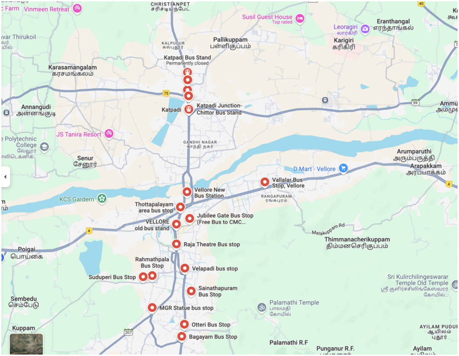
Location of identified study points in Vellore city.
Each measuring stop records measurements daily during the study interval, while vehicle estimates at 5-min intervals are stored in the traffic data, mainly collected through traffic surveys. Bike, Car, Auto rikshaw, Bus, Light, Medium, Heavy, and Trailer Trucks. Vehicle count measurements were collected from 17 stops (as detailed in Table 1) during the 2016–2023 acquisition period and are included in the full data set. Table 2 provides a concise summary of the dataset. The number of vehicles of this type that were recorded passing the measurement stop with the name ‘stop name’ during the 5-min time interval that ended at the moment indicated via the timestamp is represented by the integer variable ‘count,’ integrated into each measurement instance.
Table 1
| Stops | Latitude | Longitude |
|---|---|---|
| New Bus Stand | 12.9255746 | 79.1243371 |
| Jail Stop | 12.8822229 | 79.1061853 |
| Old Bus Stand | 12.9220972 | 79.1298299 |
| Katpadi Rly Station | 12.9716791 | 79.1354425 |
| National Theater | 12.9295309 | 79.1314584 |
| Raja Theater | 12.9145358 | 79.1299371 |
| Odai Pillayar Kovil Stop | 12.9589034 | 79.1185703 |
| CMC | 12.9254736 | 79.1345617 |
| Voorhees College | 12.9108654 | 79.1294558 |
| Chittoor Bus Stop | 12.9663375 | 79.1349161 |
| Viruthampattu | 12.9450252 | 79.1218867 |
| Tollgate | 12.8986523 | 79.1275585 |
| Roundtana | 12.9762665 | 79.2733285 |
| Vallimalai X Road | 13.0265148 | 79.1994095 |
| Thorapadi | 12.8874828 | 79.0983939 |
| Bagayam | 12.8796521 | 79.1319201 |
| Silk Mill | 12.9497813 | 79.1343584 |
List of identified stops for the data collection.
Table 2
| Date | Time | Car | Bike | Auto rikshaw | Bus | Light truck | Medium truck | Heavy truck | Trailer truck |
|---|---|---|---|---|---|---|---|---|---|
| 01-01-2023 | 08:00:00 | 26 | 32 | 12 | 5 | 3 | 4 | 2 | 4 |
| 01-01-2023 | 08:20:00 | 1 | 41 | 14 | 3 | 1 | 6 | 6 | 2 |
| 01-01-2023 | 08:40:00 | 9 | 19 | 24 | 4 | 1 | 6 | 5 | 5 |
| 01-01-2023 | 09:00:00 | 18 | 57 | 19 | 7 | 4 | 1 | 3 | 6 |
| 01-01-2023 | 09:20:00 | 18 | 4 | 12 | 11 | 2 | 1 | 4 | 2 |
| 01-01-2023 | 09:40:00 | 6 | 57 | 15 | 11 | 4 | 1 | 3 | 5 |
| 02-01-2023 | 08:00:00 | 28 | 53 | 27 | 6 | 6 | 4 | 1 | 5 |
| 02-01-2023 | 08:20:00 | 24 | 52 | 26 | 7 | 6 | 6 | 2 | 2 |
| 02-01-2023 | 08:40:00 | 3 | 39 | 11 | 2 | 6 | 2 | 2 | 5 |
| 02-01-2023 | 09:00:00 | 5 | 23 | 33 | 3 | 4 | 5 | 5 | 5 |
| 02-01-2023 | 09:20:00 | 17 | 39 | 1 | 6 | 6 | 4 | 3 | 4 |
| 02-01-2023 | 09:40:00 | 4 | 44 | 12 | 11 | 4 | 1 | 5 | 3 |
| 03-01-2023 | 08:00:00 | 12 | 4 | 23 | 10 | 5 | 5 | 2 | 3 |
| 03-01-2023 | 08:20:00 | 14 | 18 | 29 | 4 | 5 | 1 | 5 | 4 |
| 03-01-2023 | 08:40:00 | 9 | 17 | 33 | 7 | 6 | 1 | 6 | 5 |
| 03-01-2023 | 09:00:00 | 20 | 18 | 7 | 10 | 1 | 5 | 6 | 2 |
| 03-01-2023 | 09:20:00 | 21 | 44 | 7 | 4 | 6 | 3 | 4 | 1 |
| 03-01-2023 | 09:40:00 | 12 | 6 | 9 | 9 | 4 | 4 | 5 | 5 |
| 04-01-2023 | 08:00:00 | 15 | 25 | 5 | 7 | 2 | 6 | 6 | 6 |
| 04-01-2023 | 08:20:00 | 8 | 46 | 4 | 4 | 3 | 5 | 1 | 3 |
| 04-01-2023 | 08:40:00 | 3 | 18 | 14 | 2 | 5 | 5 | 5 | 1 |
A snapshot of the collected data for stopping the ‘Silk Mill’.
The distribution of traffic per day for the measurement stop ‘Raja Theater’ is displayed in Figure 2 to facilitate a better understanding of traffic patterns (Keep in mind that other traffic-measuring locations might show distinct trends). The volume of traffic typically exhibits a consistent trend. The primary significant variations occur each day, with rush hours in the morning and evening having two peaks. A weekly design is also evident, with traffic levels lower on weekends than on weekdays on specific routes, while the situation is opposite on certain routes where weekend traffic will be higher than weekday traffic, as they serve access to leisure destinations.
Figure 2
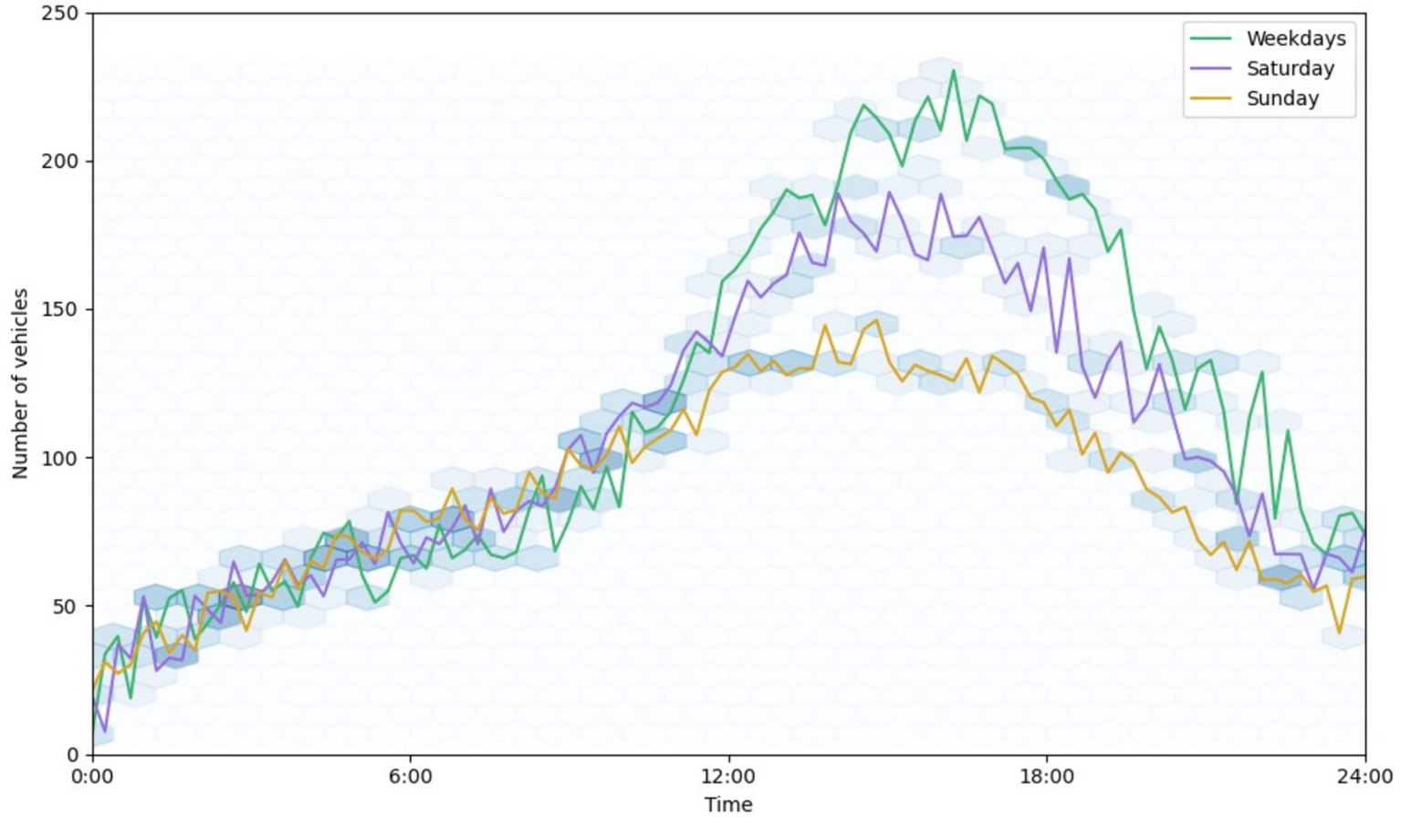
A daily allocation of vehicles at 5-min intervals was observed for the ‘Raja Theater’ stop. The average traffic volumes for weekdays, Saturdays, & Sundays are independently aggregated and shown by colored lines.
An equivalent breakdown can be seen when vehicle types are compared. Vehicle frequencies are distributed as seen in Figure 3, with certain types being more common than others. The majority of vehicles are regular passenger bikes, which are determined to be almost 320 times more common than heavy trucks. The distribution patterns vary by vehicle type, with bikes typically showing a high in the morning and evening, whereas passenger cars and auto-rickshaws exhibit separate peaks in the afternoon and evening.
Figure 3
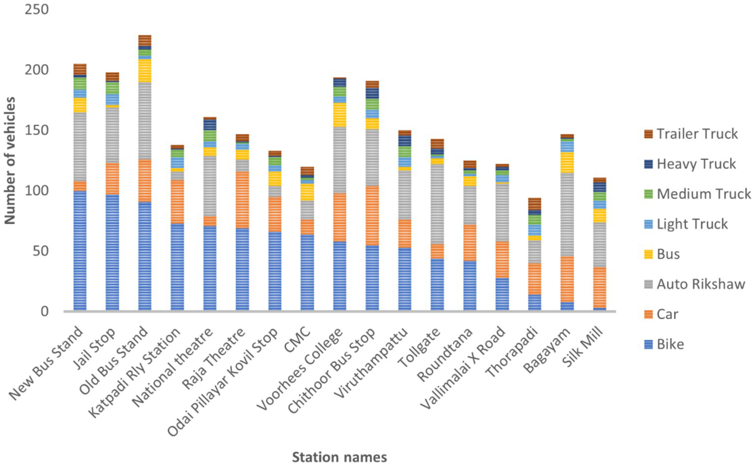
Vehicles by category and measuring stop, on average (at 5-min intervals).
Measurement errors are a natural part of the procedure. Measurement stops may have difficulties, including reporting erroneous data as a result of interruptions, or they may stop reporting data entirely in the event of a significant disruption or the data collection process at a stop being temporarily shut down.
Changes in the location of measuring stops can complicate traffic predictions. Due to ongoing building tasks or modifications in road layouts, several stops were moved either temporarily or permanently throughout the time of observation. For instance, a specific stop was converted to one exclusively for busses and auto-rickshaws while general traffic was prohibited. These modifications lead to differences in the number of vehicle types as well as the quantity of vehicles going through a stop.
Errors in the data collection process might lead to data modeling issues. One such error occurs when extremely high traffic volumes cause data overflow, preventing values from being stored. These overflowed data are excluded from further analysis.
An essential component of traffic modeling is seasonal influences. Seasonal variations can have an impact on accident rates, vehicle types, and travel habits. This impact provides valuable insights into broader trends, although it may not be detailed enough to accurately forecast occurrences that affect traffic. For example, traffic patterns can be significantly altered by a sunny season that lasts for several days or months.
The patterns of traffic are significantly impacted by public holidays as well. These periods usually see a sharp drop in traffic volume and a change in the timing of traffic peaks.
4 Methodology
A detiled explanation of the modeling framework and the error metrics used to evaluate the predictions is provided in this section. Next, a method for making predictions is described, including details on feature engineering and the machine learning models used. The flowchart of the methodology is shown in Figure 4.
Figure 4
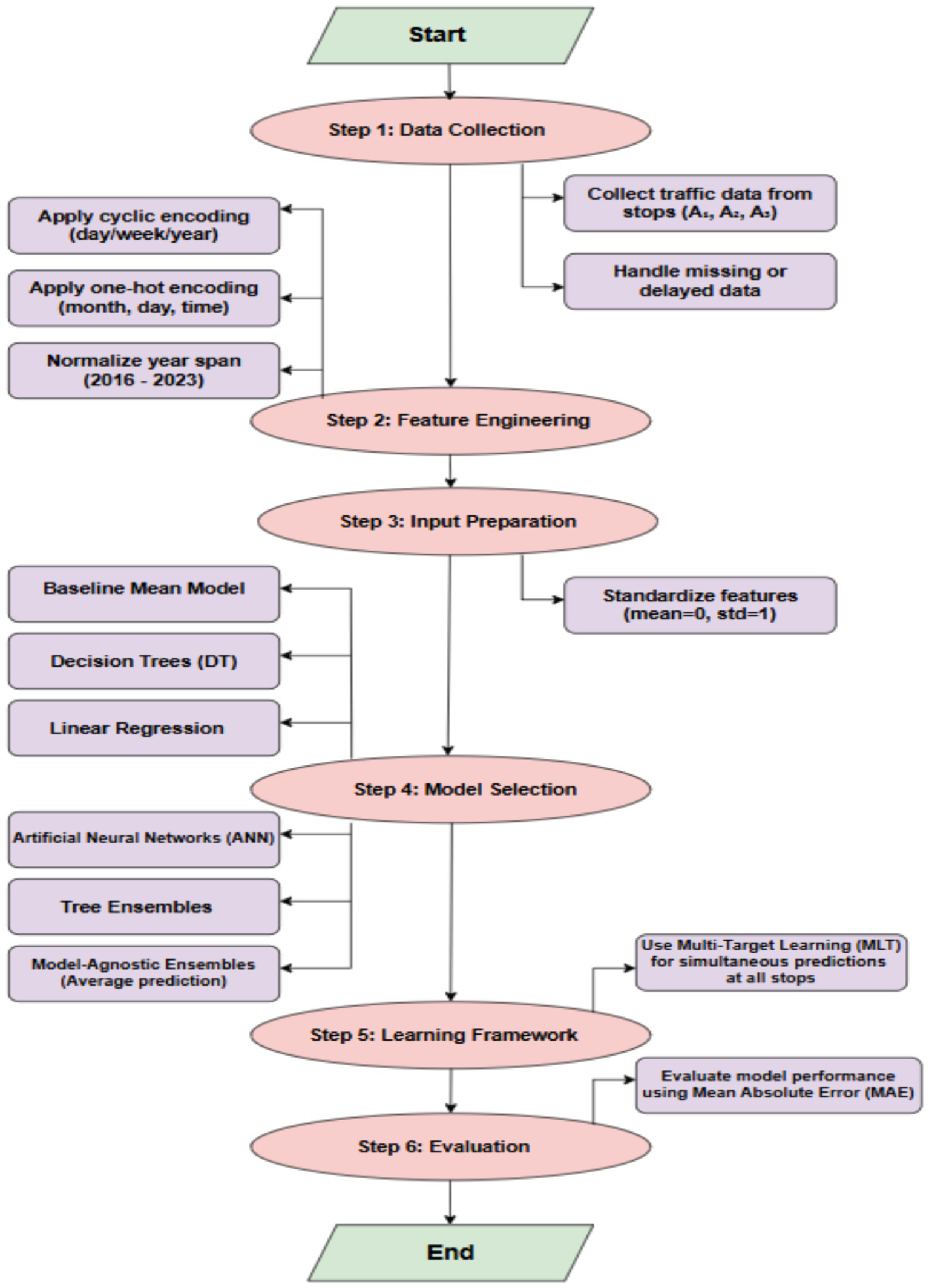
Flowchart illustrating the proposed traffic prediction methodology, including data collection, feature engineering, model selection, and evaluation.
4.1 Data collection procedure
To effectively model traffic patterns, the right approach must be chosen when many forecasts are needed for related activities, such as traffic flow forecasting. The framework of modeling for traffic prediction is presented in this section. The procedure for gathering data and creating models is shown in Figure 3. The way traffic modeling is performed is significantly affected, as the most up-to-date Past data trends are not accessible. Using traffic statistics from the last 5 min, for example, is not practical when predicting traffic numbers.
Assume that three measuring stops each have data obtained at time intervals A₁, A₂, and A₃ for stops 1, 2, and 3, respectively. Before the acquisition points, all traffic data is collected at that point. Data collection may occur at varying intervals for other stops. The gap between A₁, A₂, and A₃ and the model-building phase defines this interval, during which data is stored at a measurement stop without being considered. The data gathered up until that point is used to build a model that forecasts future traffic trends. Currently, it is possible to predict the traffic patterns for the following day. It should be noted that, in addition to data being unavailable because of delayed capture, a malfunctioning measurement stop may also be the cause of missing data. There are inherent limits to this modeling paradigm as well. The most recent data might not be available when the model is constructed because of data transfer delays (manual, for example). Standard forecasting techniques that rely on the most recent data are ineffective because this data is usually unavailable. Predictions in traditional forecasting frameworks require actual inputs like A₁, A₂, and A₃, even though the model is built using current data.
Data for this study were sourced from the local highway department, which provided foundational datasets originally compiled for urban planning initiatives. To supplement this, we identified key areas of interest and augmented the initial data with additional departmental records. Due to logistical constraints in collecting city-wide data, the scope of our analysis was initially confined to these specific, high-priority zones. We are currently developing a methodology to expand our data collection efforts to include the city’s newly developing areas. This future work will not only support urban expansion planning but also establish a critical data foundation for subsequent research phases.
4.2 Error metric
Selecting a metric that aligns with the desired predictions and goals might be difficult when optimizing vehicle number predictions (Barros et al., 2015). The chosen method for reporting all results is the mean absolute error (MAE) (Lana et al., 2018). It is defined as the metric:
The actual and expected vehicle counts at the measurement stop over a specified time period are denoted by and , respectively. It is noteworthy that the sum does not include any missing values. is a variable that represents the total number of stops. Due to its many benefits, the MAE, as shown in Equation 1, is frequently chosen over other metrics like MAPE (Schneider et al., 2017) and the MSE (Zheng and Wu, 2019; Wahab et al., 2021). Model performance can be greatly impacted by outliers (Chai and Draxler, 2014), which are frequently the result of inconsistent data. They have a less noticeable effect on the MAE, though. On the other hand, when significant prediction mistakes occur, the MSE has a tendency to severely penalize models. In certain situations, this behavior might be beneficial; however, performance degradation can occur due to data issues (e.g., distorted information or changes in traffic patterns resulting from rare events). A commonly used statistic that seeks to decrease percentage error is the MAPE. On the other hand, erroneous projections may result in severe penalties when the number of cars assessed is small. A typical example of this occurs during night traffic, when there are few vehicles on the road, and the actual count may be zero or close to it. In these cases, MAPE assigns a significant error to the predictions, even when the discrepancy is just a few vehicles. The loss functions that the models employ to reduce the mistakes must be distinguished from the error metrics that assess the accuracy of predictions. A fair comparison of the models is made possible by this study’s attempts to guarantee that the loss function used by the machine learning models matches the error metric.
4.3 Engineering features
Creating domain-dependent attributes using timestamp data is a typical procedure for creating time-dependent models in order to increase predicted accuracy (Zheng and Wu, 2019; Wahab et al., 2021). The dataset just contains the timestamp, so it’s critical to design features that machine learning algorithms can comprehend. Features constructed from timestamp data must gather information so that machine learning models can apply previously learned knowledge to new, unseen occurrences. A popular technique in time-series feature engineering is cyclic feature encoding (Schneider et al., 2017), which involves transforming time-based data using sine and cosine functions to enable periodic recurrence at a predetermined frequency. This encoding preserves periodic or cyclic events, with similar embeddings being assigned to events that are temporally close. Furthermore, the algorithm’s performance is improved by incorporating one-hot encoded time features. This method simulates the separate effects of events that occur near one another but are not comparable (Khadiev and Safina, 2019). Additional information that would be missed by cyclic feature encoding alone is captured by this encoding technique. The features that were taken from each 5-min measurement interval’s date and time data are shown in Table 3. The standardized mean of zero and standard deviation of one for all generated features helps some algorithms, like neural networks, converge while having no effect on others, like tree-based models.
Table 3
| Type of feature | Count | Summary |
|---|---|---|
| Monthly One-Hot Encoded | 12 | For every month of the year, a vector of binary values is used. |
| Day of the Week with One-Hot Encoded | 7 | Every day of the week has a binary vector. |
| One-Hot Encoded Minutes | 72 | A binary vector for each 5-min interval within a day. |
| Cyclical Day Features | 2 | Cyclic time encoding with a daily cycle. |
| Cyclical Week Features | 2 | Cyclic time encoding with a weekly cycle. |
| Cyclical Year Features | 2 | Cyclic time encoding with a yearly cycle. |
| Normalized Year Span | 1 | A normalized time span from 2016 to 2023, scaled between [0, 1]. |
Overview of feature types, dimensions, and explanations (2016–2023).
4.4 Models
Accurately modeling traffic using features derived from timestamps is a complex task. This section provides an overview of the models applied in traffic modeling, highlighting their respective strengths and weaknesses. It is worth mentioning that more advanced machine learning techniques, detailed in Section 2, can be applied for real-time traffic forecasting. These techniques use temporal dependencies, often known as lag characteristics. They are not appropriate in this situation, though, because of the nature of the data collection procedure described in Section 4.1. Since the most recent traffic data is not available at the time of prediction, temporal data cannot be used to make the forecast.
We chose Single-Task Learning (STL) and Multi-Task Learning (MTL) models for our urban traffic dynamics study because they fit our objectives and the features of our dataset. For targeted studies, STL models are beneficial since they let us identify and investigate the impact of particular elements on traffic circumstances, including weekend changes. Their straightforward structure also facilitates easier interpretation and helps establish initial performance metrics.
On the other hand, to better represent the multifaceted and interdependent aspects of urban transport systems, MTL models play a vital role. These models are capable of learning from several related tasks at once, such as predicting traffic flow and estimating travel duration, by drawing on commonalities across different data streams. This shared learning improves model generalization, especially when working with limited datasets, and offers a more resource-efficient alternative to training separate models for each task. By incorporating both time-series traffic data and contextual factors like weekday-weekend classification, MTL helps construct a more comprehensive view of urban mobility. This dual approach allows us to begin with narrow investigations and progressively expand our analysis as more data becomes available.
We also implemented linear regression techniques owing to their foundational simplicity and low computational overhead. A significant benefit of this method is its transparency; coefficient values directly reveal how specific inputs, such as whether a day is a weekday or weekend, influence traffic behavior. Urban transport planners seeking to understand and address congestion patterns will find this clarity helpful. Furthermore, linear regression provides a reliable starting point for determining the main patterns in our initial dataset and lays the groundwork for further research with more complex models.
A general classification of the machine learning models used is single-target learning (STL) and multi-target learning (MTL). Assuming that the aims are independent, the STL framework suggests that the flow of traffic at one stop has no bearing on the flow at other stops. The creation of distinct models, each aimed at forecasting traffic at a particular stop, is necessary when stops are regarded as independent. The ability of MTL models to forecast several targets at once allows them to capture target dependencies, which can enhance generalization in contrast to STL models. This method entails building a single model that forecasts traffic simultaneously at every measuring site. In this work, we use MTL models, which eliminate the need to create individual models for every traffic stop, thus simplifying the construction and training process.
Taking into consideration these restrictions is crucial while selecting models. Hence, the focus is on models that satisfy these two essential requirements: (a) the model can be trained effectively and in a manageable amount of time (a couple of hours, for example), and (b) it is simple to update the model with new data. Popular machine learning techniques, such as Random Forest and XGBoost, are not considered because of the aforementioned constraints. Despite being widely used for tabular data, these models have several drawbacks:
-
They are not optimal for simultaneous multi-target predictions (multi-target learning is not supported by all XGBoost executions, at least not during testing and writing, to prevent the prediction of traffic across multiple stops);
-
They cannot deal with missed outputs in situations involving several targets.
-
They need a complete model rebuild instead of permitting partial updates as new data is introduced; and
-
Their limited ability to select optimization objectives results in performance issues when using MAE.
4.4.1 Tree-specific ensembles
The predictions of several decision trees are combined after they have been trained in order to improve the forecast accuracy of a single tree (Ho, 1995). A process like this is frequently referred to as a random forest. A random forest uses a technique known as bootstrap aggregation to train individual trees on training data that is randomly selected with replacement (Breiman, 1996). Numerous DTs make up a random forest. The trees are typically constructed using deterministic methods, which often produce trees that are similar. Individual trees are usually trained on randomly chosen dataset segments or with randomly picked features in order to encourage variety within the ensemble. Similar to classic tree ensemble methods, Extremely Randomized Trees (Geurts et al., 2006) is a comparable technique in which attribute splits are chosen at random. This method’s main advantage is its computational efficiency, which results from the nodes being divided using reduced criteria.
4.4.2 Mean at baseline
A straightforward model for traffic flow on a road segment forecasts the average volume of traffic at a particular measuring stop without taking time into consideration. Despite its inability to account for recurring fluctuations in traffic volume, this model provides a standard against which more complex models can be evaluated.
4.4.3 Decision trees
To create interpretable predictive models, DT learning (Kotsiantis, 2013). A straightforward and powerful machine learning technique is used. The information is automatically converted into a decision tree (DT), with the terminal nodes predicting the desired value and each branch representing an attribute test.
DT can be constructed using a variety of techniques (Mehedi Shamrat et al., 2022), such as ID3, C4.5, CART, CHAID, and MARS. These approaches distinguish ways that discrete and numerical information is transmitted, as well as how the branch-building process is carried out. Randomness can be incorporated when the features are equally important. However, most of these methods are deterministic. Although DT can usually be constructed quickly, deciding how to create branches can take a considerable amount of time, mainly when loss functions like MAE are used, as they necessitate sorting node values.
4.4.4 Regression analysis with linear
The independent and dependent variables’ linear correlations are modeled utilizing linear regression (LR), which uses learning coefficients. It enables effective optimization and offers good interpretability. A distinct LR model is created for each stop to forecast traffic flow, and it is trained using MAE loss instead of MSE loss to better align with the challenge’s goals. To introduce non-determinism into the training process, the LR weights are iteratively updated using stochastic gradient descent. A baseline model that works well in circumstances where only linear relationships are considered is the LR model.
4.4.5 Neural networks
To identify intricate and nonlinear correlations between dependent and independent variables, mathematical models known as artificial neural networks (ANNs) are frequently employed. Neurons are organized into individual layers of specific sizes to form a neural network. A more intricate network that can approximate nonlinear functions can be created by stacking these layers. Once a neural network is constructed, it must be trained to find the mapping between input and output data. Backpropagation is the most popular method for this (Rojas, 2013), wherein we minimize the loss function by using gradient descent and iteratively changing the weights of different layers. This research focuses on fully connected neural networks, even though neural networks come in a variety of configurations and are frequently tailored for particular domains (Devlin, 2018; Li et al., 2021).
4.4.6 Agnostic ensembles for models
The sets of different models for machine learning, known as model-agnostic ensembles (Dong et al., 2020; Zhou and Zhou, 2021) are used to combine knowledge through different techniques, making predictions that are more accurate and dependable. The various ways predictions combine depend on the problem type, such as classification or regression. Combining weighted predictions yields a more precise estimate for regression problems. The ensemble’s algorithm performance can determine the weights of the various models, or all forecasts can be given the same weight. The ultimate prediction in the latter scenario is determined by averaging the projections from each individual model. The second method, which is straightforward, is used by merely averaging the predictions. In this work, neural networks are combined using only model-agnostic methods.
5 Results and discussion
The models, configurations, and hyperparameters are first introduced in this part, and the impact of various hyperparameters on prediction accuracy is illustrated. Once the model that performs best on the validation set has been identified, its performance on the test set is examined. The impact of various occurrences is evaluated, and the model’s performance for each measuring stop is reviewed. It also looks at how performance evolves with time. The effect of public holidays and rush hour is an example of an interesting trend in the data that is highlighted by the selection of specific times and monitoring places. But not every measurement site exhibits these clear trends.
5.1 Details of the experimental design and implementation
The models’ performance on new, unseen samples is assessed by dividing the data into training and test sets. The model is then trained using these sets, and its performance is evaluated using them. The temporal sequence must be maintained when splitting the data into two groups, and the most recent observations that do not overlap with the training data must be included in the test set (Cerqueira et al., 2020). Four-split time-series cross-validation is used to address this. Figure 5 illustrates how the data were separated for analysis. Please be aware that every model is stochastic by nature. For a more precise and reliable evaluation of their achievements across various datasets and parameter settings, we repeat the training procedure 30 times for every combination of train/test split and hyperparameters.
Figure 5
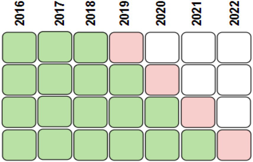
Temporal division of the data into four training (green) and testing (red) sets through 4-fold cross-validation.
The best model and the most suitable set of hyperparameters for that model must be chosen when selecting and evaluating models. To avoid inflated performance estimates during the hyperparameter tuning process, do not use test data to ensure an accurate evaluation of the models. Models were constructed and chosen using nested cross-validation (Wainer and Cawley, 2021). Using this method, each training set was split into two sections: a validation set to identify the most effective hyperparameters and a training set to train the models with various hyperparameter settings.
Finding the ideal neural network architecture is usually a complex undertaking since it requires a lot of computation and the use of several tuning techniques (Akiba et al., 2019; Victoria and Maragatham, 2021) to identify the best hyperparameters. The hyperparameters explored during the model-building process are described in Table 4. To generate 20 models for every combination of hyperparameters and train/test split, we conducted a basic grid search across all conceivable parameter value combinations. In the next section, we report the findings for each combination of hyperparameters and demonstrate how specific models’ performance is impacted by them. Only the model and hyperparameters linked to the highest accuracy on the validation set would be chosen for real-world applications, such as daily use.
Table 4
| Model type | Hyperparameter | Values |
|---|---|---|
| Neural network | Number of Layers | {1, 2, 3, 4, 5} |
| Neuron Count per Layer | {128, 256, 512} | |
| Dropout Rate | {0, 0.2} | |
| Early Stopping Patience | {5} | |
| Decision Tree | Max Depth | {2, 4, 6, 8, 10, None} |
| Min. Samples per Leaf | {1, 2, 3, 4, 5} | |
| Extremely Randomized Trees | Max Depth | {2, 4, 6, 8, 10, None} |
| Min. Samples per Leaf | {1, 2, 3, 4, 5} | |
| Linear regression | Optimizer | {SGD} |
Ranges of hyperparameters explored through grid search.
Every pair of split and hyperparameter train/test combinations was subjected to 30 separate runs of each method on an AMD Ryzen Threadripper PRO 5975WX. Python 3.10 was used to implement the algorithms. The models were trained with the PyTorch framework (Paszke et al., 2019) and PyTorch Lightning (Falcon, 2019). The analysis was carried out using Snakemake (Mölder et al., 2021) and scikit-learn (Pedregosa et al., 2011).
5.2 Selection of models
Several limitations must be balanced when developing and evaluating models. These constraints include factors such as the time required for model construction and training, the model’s overall complexity, its inference efficiency, the need to adjust hyperparameters, and other challenges, including adapting models to new data. Four distinct train/test splits of the data, as explained in Section 5.1, were used to train and assess the models outlined in Section 4.4. First, we experimented with different model types, such as neural networks, decision trees, and random forests, and tuned their hyperparameters. A comparison of the various model types based on the MAE between the observed and expected number of vehicles is presented in Figure 6. The models with the best hyperparameter values identified by the validation set are shown here. The standard deviation of performance across 30 repeated runs is represented by the gray bars. The study shows that all models perform better than the benchmark baseline model, which forecasts the mean, for an MAE of roughly 45.
Figure 6
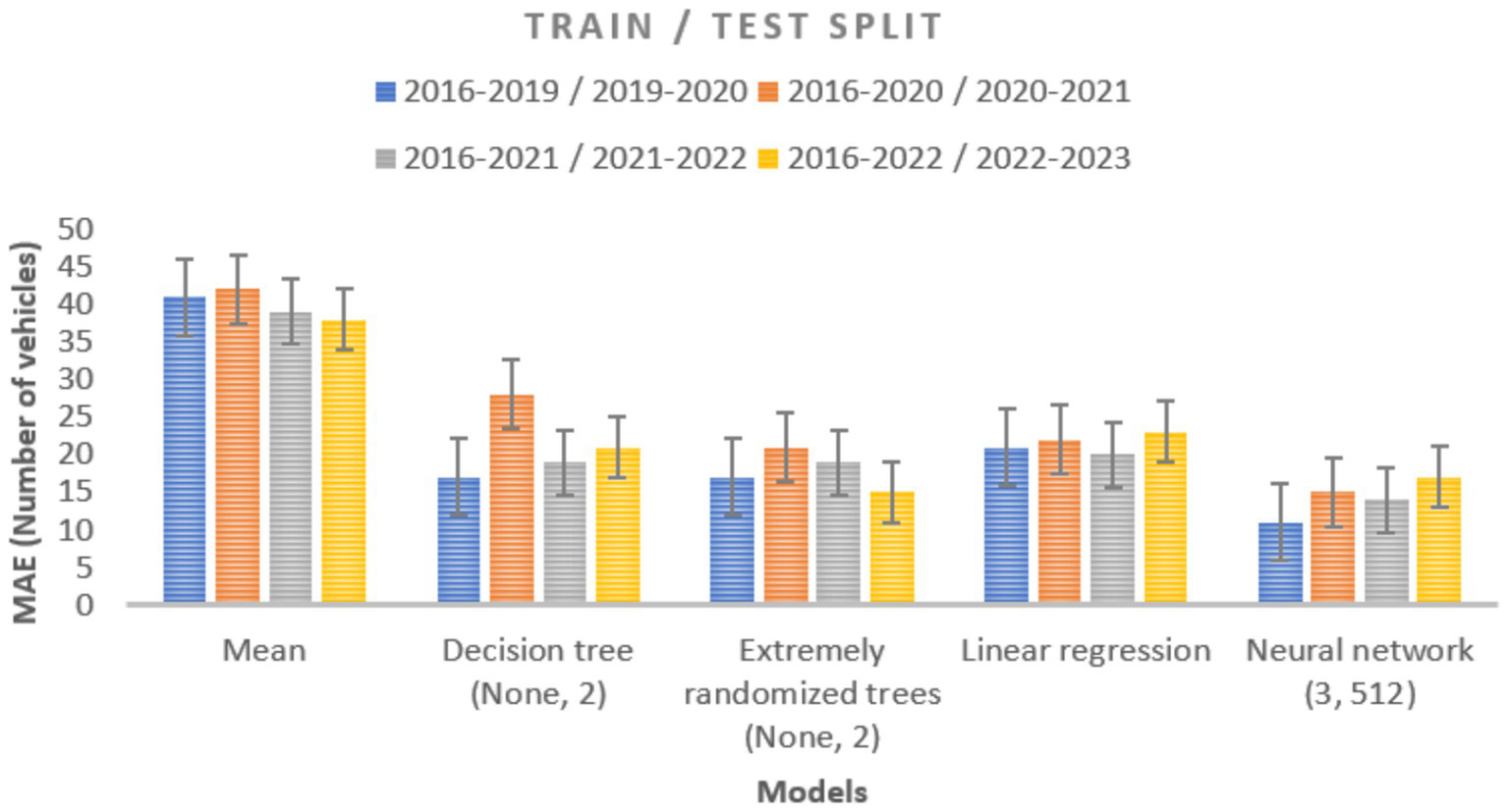
Using data from a prior year, the MAE compares the observed and anticipated vehicle counts for several machine learning models. Four different train/test splits were used to train and assess each model 30 times. The standard deviation, illustrated by the gray bars, shows the variability in performance.
When compared to a naive baseline, the error of the tree-based models is almost half, indicating that they perform well in terms of prediction. In both approaches, when the tree depth is unrestricted and every leaf has a minimum of two samples, we obtain the best hyperparameters from the validation data. Across the years under consideration, their performance is found to vary substantially, with 1 year showing a noticeably larger inaccuracy than the others. There is a significant difference in performance between runs of the same dataset since both tree models are stochastic. It is almost twice as accurate as the baseline for linear regression. Linear regression exhibits significantly more stability over the years taken into consideration than tree-based models, with no discernible declines in performance in any 1 year. Repeatedly training linear regression on the same data yields significantly higher consistency, with minimal variation between runs. As a result of their consistently higher performance over other methods, neural networks are considered the best models. Furthermore, the predictability of the results is maintained with remarkable consistency across a range of experimental runs and the years under study. Three hidden layers, each with 512 neurons, are found to be the ideal arrangement in this case. Neural networks consistently outperform all other models, even when inadequate hyperparameters are used. It remains unclear why neural networks outperform conventional tree-based models. This advantage is likely due to the large volume of available training data and the neural network’s ability to learn complex decision boundaries. As a result, there is growing interest among researchers in applying neural network-based models to traffic modeling, as these models often outperform traditional approaches, even when hyperparameters are not perfectly optimized. Although the dropout rate (Kotsiantis, 2013), is a common neural network hyperparameter, it is not discussed in this context, as it did not lead to any noticeable improvement in the performance of the evaluated models.
The impact of neural networks’ hyperparameters on the training process is further examined, as these networks are considered more suitable for traffic flow prediction in our context than other approaches. The impact of various hyperparameters on traffic flow prediction performance is illustrated in Figure 7. It has been discovered that performance is greatly impacted by the parameters chosen. With an MAE of about 30, networks with a single hidden layer usually perform poorly because they are unable to capture all the information. It has been demonstrated that increasing the number of hidden layers, and consequently the total number of parameters, improves neural networks’ predictive accuracy. The network with three hidden layers and 512 neurons each performed the best out of all the models that were evaluated. The usefulness of this architecture, as mentioned in the preceding section, was confirmed by the consistent outcomes it produced throughout the test and validation datasets.
Figure 7
![Bar chart showing Mean Absolute Error (MAE) in vehicle counts for various neural network models with different layer and neuron configurations. Four datasets are compared: [2016-2019]/[2019-2020], [2016-2020]/[2020-2021], [2016-2021]/[2021-2022], and [2016-2022]/[2022-2023]. Each configuration shows similar performance across datasets.](https://www.frontiersin.org/files/Articles/1631748/xml-images/frsc-07-1631748-g007.webp)
For neural network models, the MAE between the actual and forecast vehicle counts is calculated using data from years that have already been observed, with different hyperparameters such as the number of hidden layers and their sizes. Every model underwent 30 training and testing sessions in 4 distinct train/test splits. For the performance, the gray bars show the standard deviation.
5.3 Ensembles of neural networks
Now, neural network ensembles are the focus. Machine learning forecasting accuracy can be improved by mixing forecasts from several models, as is well known. A comparison of an ensemble approach using 15 neural networks and regular neural network models is shown in Figure 8. To allow each neural network in the ensemble to learn different information, we initialize and train them separately. The process of forming an ensemble is always advantageous and frequently results in additional gains in prediction accuracy. Neural networks with three hidden layers and 512 neurons each make up the most efficient ensemble structure, as was previously established. As the complexity of the models inside the ensemble increases further, no performance improvement is seen.
Figure 8
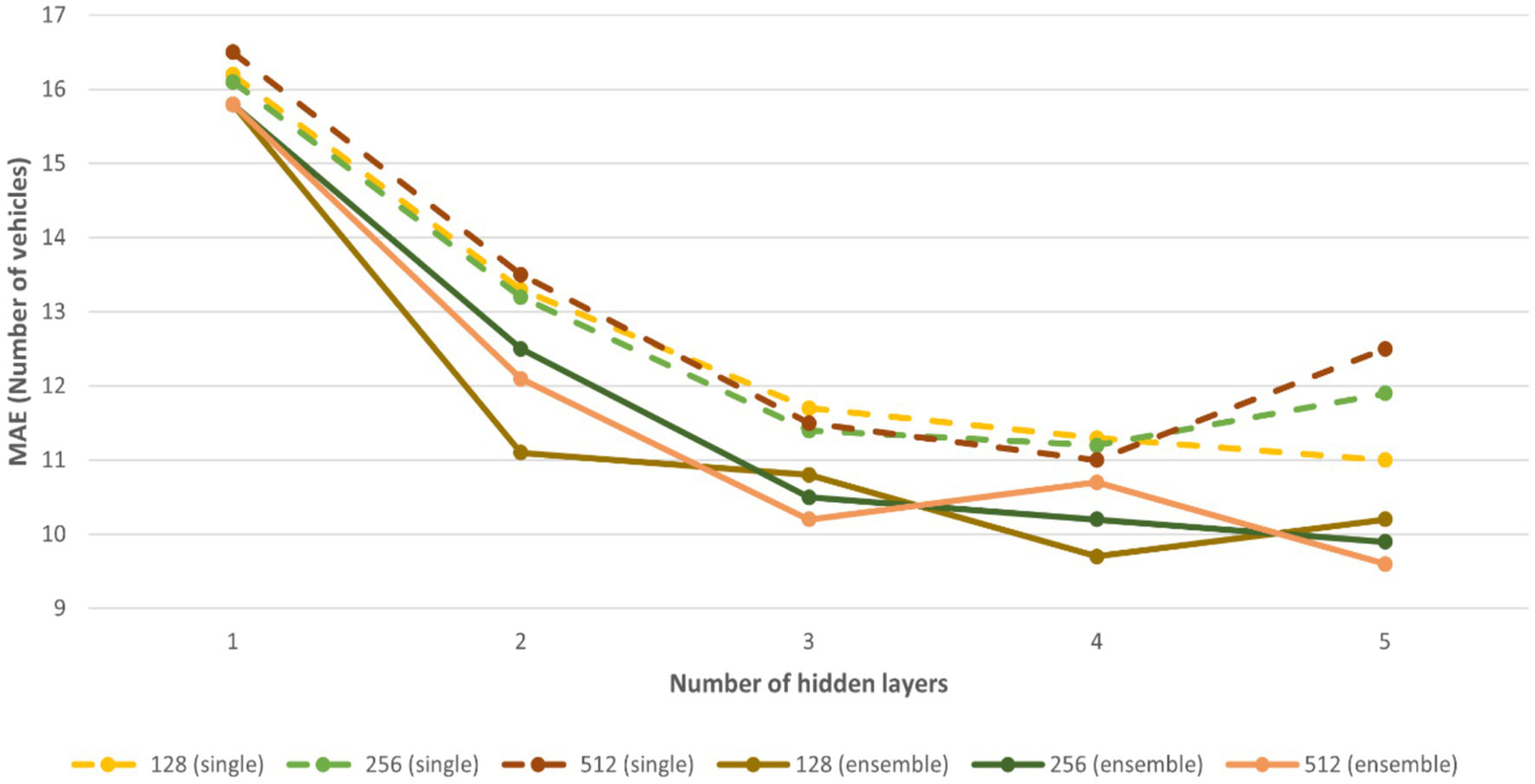
Evaluation of the impact of architectural changes on the MAE is possible by varying the number of hidden layers (from 1 to 5) and their sizes (128, 256, and 512 units) in both ordinary neural networks and ensemble models.
5.4 Duration of training
As traffic data changes, regular updates may be required, which may be a time-consuming operation, so cutting down on model development time is essential. The training and prediction times for each model are shown in Table 5. However, as described in Section 5.1, different train/test split sizes prevent direct comparisons across all folds. A single train/test split from 2019 is hence the main emphasis. The stated statistics are all averages over the 30 runs. The different model types are shown to have dramatically varying training times. Despite the lack of high precision, it is possible to quickly train a baseline model that accurately predicts the mean traffic at a particular stop. Although they are more computationally expensive, tree-based models offer higher accuracy. A comparison between extreme trees and a single decision tree reveals that training an ensemble of trees uses more processing power. The models that cost the most to compute are neural networks and ensembles constructed on top of them. The time required for their construction is heavily influenced by the size and architecture of the network. Longer prediction lengths and slower training times are typically linked to deeper and broader networks, as one might anticipate. This network requires the most computing power to train, comprising five hidden layers with 512 neurons each. Although their training times are not included in Table 2, it should be noted that the amount of time needed for ensemble training is usually related to their size. The training period is typically 10 times longer when ensembles of 10 neural networks are taught consecutively. Since the training duration of neural networks with Dropout is similar to that of networks without Dropout, we did not include them in the list.
Table 5
| Type of model | Training time (sec) | Inference time (sec) |
|---|---|---|
| Decision Tree (None, 2) | 0.19 | 0.01 |
| Extremely Randomized Trees (None, 2) | 125.68 | 0.16 |
| Neural Network (128 units, 1 layer) | 23.79 | 0.06 |
| Neural Network (256 units, 1 layer) | 145.51 | 0.57 |
| Neural Network (512 units, 1 layer) | 229.69 | 0.30 |
| Neural Network (128 units, 2 layers) | 236.93 | 0.31 |
| Neural Network (256 units, 2 layers) | 266.45 | 0.32 |
| Neural Network (512 units, 2 layers) | 655.69 | 0.52 |
| Neural Network (128 units, 3 layers) | 655.69 | 0.57 |
| Neural Network (256 units, 3 layers) | 642.70 | 0.59 |
| Neural Network (512 units, 3 layers) | 819.35 | 0.74 |
| Neural Network (128 units, 4 layers) | 820.70 | 0.87 |
| Neural Network (256 units, 4 layers) | 899.02 | 1.86 |
| Neural Network (512 units, 4 layers) | 930.53 | 1.47 |
| Neural Network (128 units, 5 layers) | 1,080.80 | 2.08 |
| Neural Network (256 units, 5 layers) | 1,293.85 | 2.64 |
| Neural Network (512 units, 5 layers) | 1,263.38 | 1.54 |
| Neural Network (128 units, 5 layers) | 1,486.36 | 2.45 |
| Neural Network (256 units, 5 layers) | 1,510.61 | 3.40 |
Training and inference times for various machine learning models.
5.5 Examining the forecasts
An ensemble of 10 neural networks, each with three hidden layers and 512 units, was identified as the best-performing model after analyzing the previously presented accuracy results. Based on the completed models, Figure 8 illustrates the distribution of prediction errors, which represent the difference between actual and anticipated values, for a few selected measurement points. From the figure, we can identify two key observations: specific measuring stops are more challenging to forecast traffic levels more accurately than others. Because daily traffic variances on popular roads are larger than those on less busy roads, it is challenging to anticipate traffic volumes at these sites. The figure shows the existence of outliers in the prediction errors. The majority of projections turn out to be accurate; however, mistakes of magnitude 100 or higher are common. These notable inaccuracies are frequently ascribed to exceptional occurrences that the current models are unable to adequately represent.
A more thorough analysis of how the predictions of the chosen model match the actual data is shown in Figure 9, which presents a thorough comparison. Each point represents the flow of traffic at either 6 AM or 8 AM. A clear divergence between weekdays and weekends is the first noteworthy pattern that is noticed. Compared to weekdays, weekend traffic is less frequent and less variable, which results in relatively fewer forecast inaccuracies. When this shift takes place, the frequency of the vehicles will be drastically changed. The chosen model is able to forecast and account for this shift in traffic distribution.
Figure 9
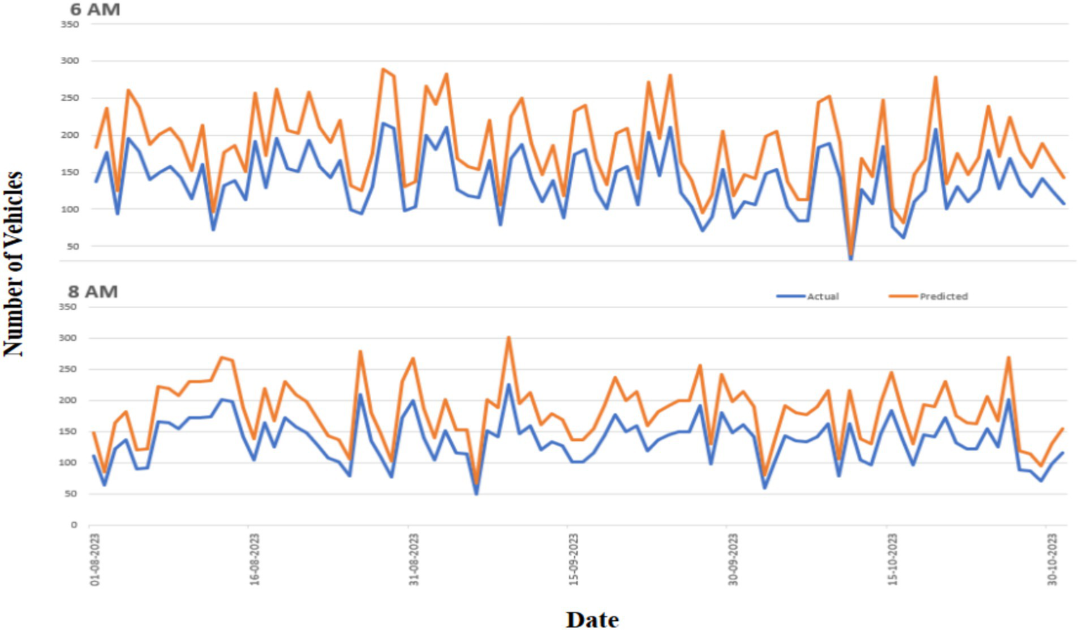
Actual (blue) and expected (orange) vehicle counts at stops during August through October are displayed in the test data. Measurements were made at 6:00 AM (top) and 8:00 AM (bottom) at 5-min intervals. The actual number of vehicles, as determined by the Neural Network (NN) model (3,512), is represented by the blue line, while the orange line indicates the anticipated number.
Despite the rigorous selection of this sample, several intriguing conclusions can be made. First, daily traffic patterns, such as the morning rush hour and the slower traffic on weekends and evenings, are well-represented by the model. As a result, it is possible to learn and use the training data’s predictable periodic patterns to anticipate future traffic levels. A more troublesome trend that the model finds difficult to capture is the change in traffic quantities. The model consistently underestimates the traffic volumes in the test group, as the example illustrates. It supports the notion that traffic volumes have grown over time at a particular monitoring stop. The most recent test data can consequently have an entirely distinct distribution from the training data because it only contains the most recent measurements. The model frequently overestimates or underestimates traffic flow, which raises the possibility of abrupt variations in traffic volumes. However, because real-time data is not available, the model regularly generates skewed predictions. To account for this transition and produce more accurate estimates, the models will likely use the most recent traffic count statistics. Unfortunately, these characteristics are not included in the model by the current data transfer method.
The actual measured values and anticipated values for the stop at Chittoor Bus Stop during 4 days are shown in Figure 10 to provide a more thorough explanation of the errors. Although the predicted values in this instance represent the general traffic patterns without being overfitted to the noise, the observations are perceived as being somewhat noisy between the 5-min intervals as shown in Figure 11. Despite the lack of representations for each stop and time period, the models continuously provide precise traffic distribution estimation across different locations and intervals, excluding noise and random oscillations. The examination of data drift on test data is shown in Figure 12, which shows how the prediction error changes over a year without any model upgrades or retraining. Using data pooled across all available monitoring stops for every day over the next year, the MAE is calculated by comparing the measured and forecasted vehicle numbers. The MAE in this figure cannot be directly compared to the MAE in other figures since we did not include measurement stops with missing data. The pattern revealed by the linear trend persists over time despite the noisy nature of the single aggregated daily error. This illustrates a significant trend, showing that traffic patterns evolve over time. Performance is likely to deteriorate if the model is not updated on a regular basis. In addition, a clear, jagged line is seen all year long. Variability during the week and increased traffic numbers are the causes of this pattern. Therefore, forecasts for weekdays are linked to higher MAE values. For example, Figure 11 shows a visual comparison of the analysis between the actual data and the predicted values for an identified stop.
Figure 10
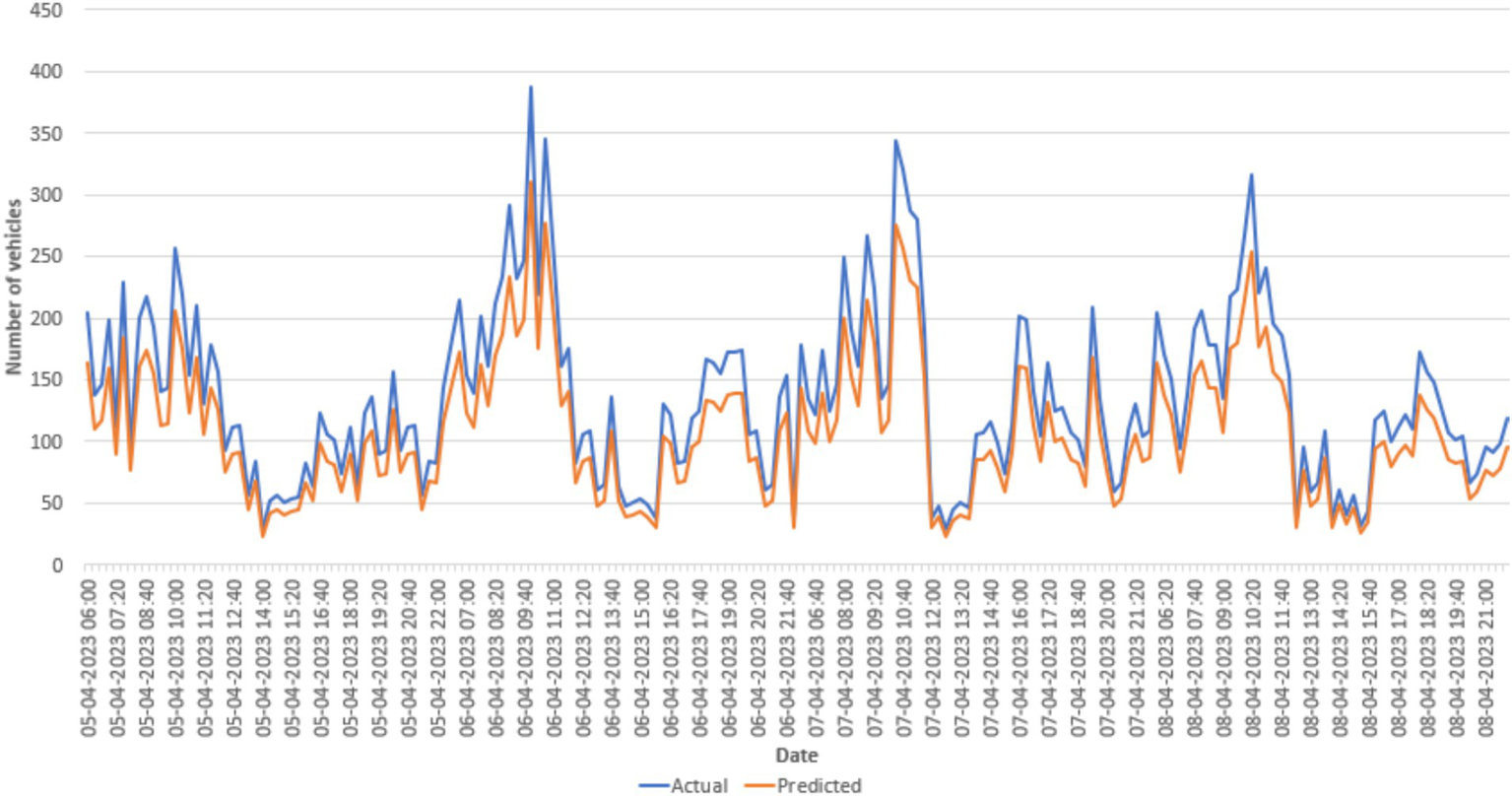
Test data displaying actual (blue) and predicted (orange) traffic across 4 days using the Neural Network (3, 512) model.
Figure 11
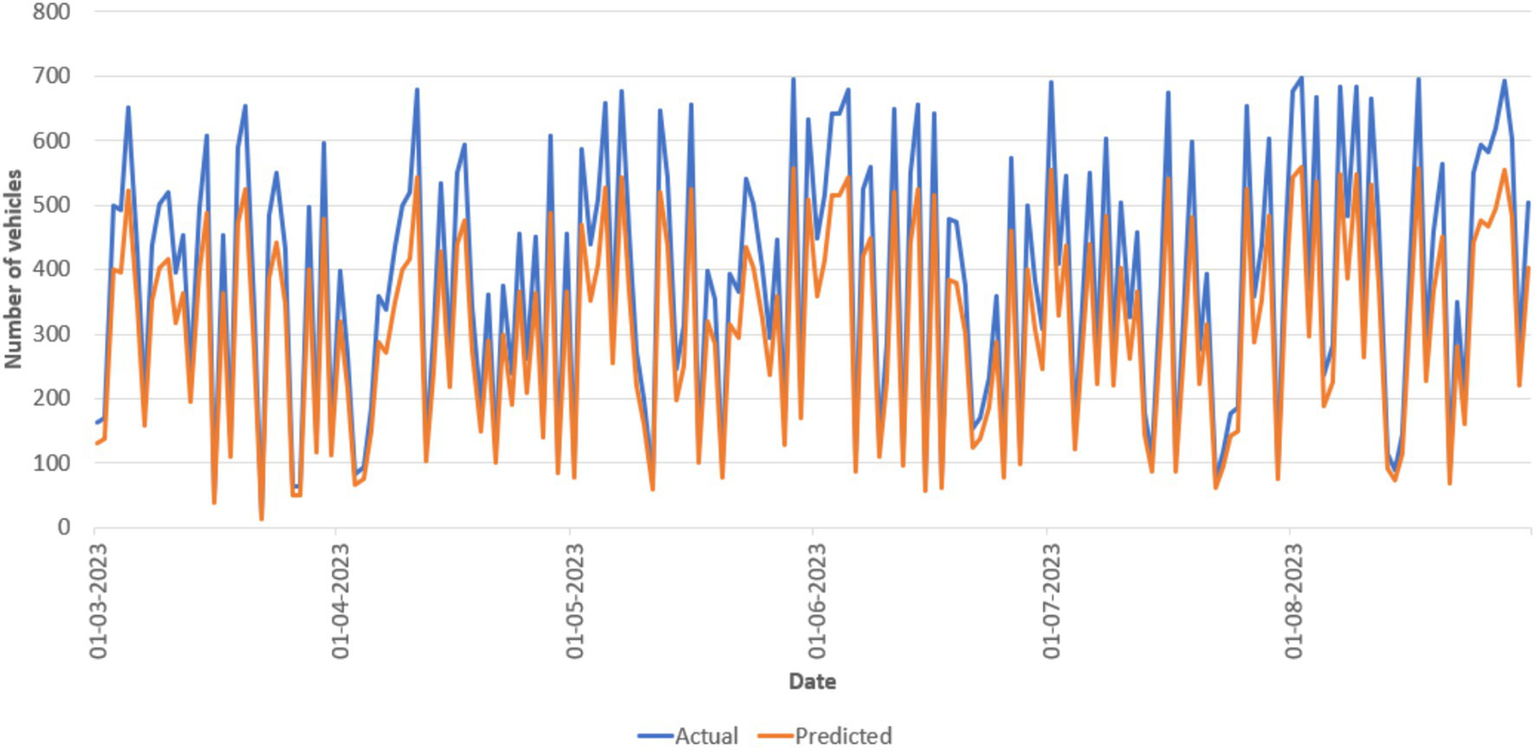
Actual traffic (blue) and expected traffic (orange) for stop names during 3 weeks are visualized using the Neural Network model (3,512), with vehicle count forecasts.
Figure 12
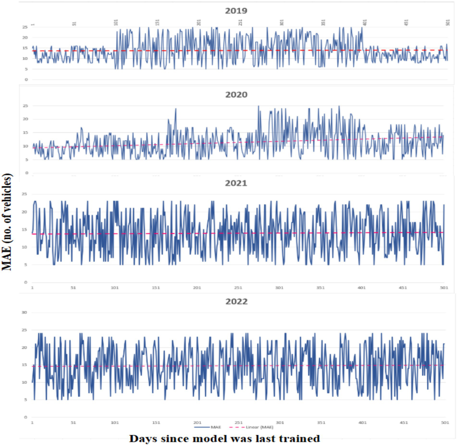
Over a period of 365 days, the MAE is calculated daily, demonstrating a progressive decline in predicting accuracy. As the time horizon increases, the forecast model’s reliability decreases, as seen by the interpolated linear trend.
Important clarifications regarding the meaning of the several feature types used for prediction are finally given. Three different feature categories are introduced, as explained in Section 4.3. The feature categories are derived from times and dates, the presence of holidays, and seasonal information. When integrating all three feature categories, the optimal ensembles in Section 5.3 produce an MAE between 10 and 12. The significance of the feature groupings varies, though. While elements that indicate holidays and seasons have a much lesser impact on the prediction, those that are based on date and time are thought to be the most crucial. The best ensemble’s MAE barely increases by 3% when it is retrained without the additional features. The MAE also rises by roughly 3.5% when the ensemble is trained without weekend data, using only date/time and other factors. The significance of different data points and weekend aspects cannot be disputed, even though the overall MAE decreases by only a few percent in their absence. These factors significantly improve predictions during severe seasonal events or holidays. To put it another way, weekend circumstances and other parameters can dramatically increase model accuracy for unexpected events, but the overall MAE summary does not consider this improvement because these events are uncommon.
5.6 Further study and next steps
While trying to compare the approach and results arrived at in the study with other similar research articles as cited in (Petelin et al., 2023) gives a very similar outlook on the mobility analysis. Taking these as inputs, we will have to extend the study further to a broader spectrum to cover other parameters like the ones highlighted below and derive more detailed outcomes from the analysis.
This initial research aimed to understand how a city’s growth, increasing population, and evolving vehicle conditions have transformed its transportation landscape. During our study, we identified several additional factors that significantly impact daily commutes, including vacation seasons, holiday crowds, traffic jams, VIP escorts, and seasonal weather variations, notably high summer temperatures.
The next study effort should be centered on more thorough data collection, analysis, and methodology as a result of these discoveries. The goal is to uncover intricate patterns of traffic and road commutes within the city. This current paper provides the foundational insights necessary to build that broader study. A more thorough examination of these affecting elements will be possible if the next phase concentrates on specific regions rather than the entire city.
The cumulative results of the studies will eventually guide local authorities in urban planning and traffic management, primarily to support outlier scenarios that are influenced by seasonal parameters. This study will lay the foundation for further detailed studies involving other parameters as highlighted above and eventually help identify patterns and predict outcomes that will aid in effective urban development and seamless traffic management.
6 Conclusion
This study presents a new dataset that monitors traffic flow for a variety of vehicle types on several road routes in Vellore, from 2016 to 2023. Five-minute intervals are used to count and classify vehicles.
To make predictions, models are constructed using this dataset that integrates traffic data and information on weekends, without relying on temporal relationships. This criterion is crucial since real-time data is not always collected, and the most recent past is insufficient to produce accurate projections of vehicle flows. It is shown that adequate feature engineering can provide usable models in spite of current constraints. The ability to recognize and take into account a variety of variables and trends that affect traffic flow makes these models useful for traffic prediction. They are therefore helpful instruments for short-term planning and well-informed traffic management, enabling informed decision-making. Neural networks achieve a better balance between prediction accuracy, inference, and training time, and the ease of making incremental modifications than conventional linear and tree-based models. A comparison of several models and the impact of hyperparameters on their performance forms the basis of this finding. The benefits of merging several models are also examined, as this can result in improved accuracy, but it also introduces the drawback of greater computing complexity.
The simplified predictive framework developed in this research offers a practical and immediate solution for Vellore’s traffic management authorities. By relying solely on traffic flow, vehicle count data, and the distinction between weekdays and weekends, city administrators can deploy these models without needing extensive investments in sophisticated data collection infrastructure, such as weather sensors or public holiday databases. The models can be integrated into a real-time traffic monitoring system to forecast congestion hotspots several hours in advance. For example, knowing that a particular road segment is likely to experience high traffic on a weekday afternoon allows traffic police to pre-emptively reroute traffic or deploy additional personnel to manage the flow. This proactive approach, driven by easily obtainable temporal data, can significantly reduce commute times and enhance road safety without requiring a complete overhaul of the city’s current traffic management tools.
Furthermore, the insights from this study can inform long-term urban planning and policy decisions. The models can simulate the impact of new infrastructure projects, such as a new flyover or a change in traffic signal timing, on the overall traffic network. By analyzing the weekday versus weekend patterns, planners can identify systemic issues that require structural changes, such as inadequate public transportation during peak commute hours or insufficient parking near commercial centers on weekends. This data-driven approach to planning ensures that resources are allocated effectively, addressing the root causes of congestion and promoting sustainable urban mobility. The research provides a blueprint for other rapidly growing cities with limited resources, demonstrating that effective traffic solutions can be built on a foundation of minimal, yet meaningful, data, thereby democratizing access to advanced traffic management strategies.
To understand the circumstances under which the model performs well and the regions where precise traffic flow predictions are lacking, the top-performing model is examined. For the majority of the measuring stops, we show that our projections are generally correct. Some situations, however, are proven to be more challenging to represent. Examples are given of weekends when traffic can fluctuate wildly and the changeover to summer time. Furthermore, it is demonstrated that the models often overestimate or underestimate traffic flow and that data drift may eventually cause them to perform worse. Consequently, it is essential that models be modified frequently to incorporate fresh data.
The deeper analysis of features, their construction, and the quantification of their importance are areas that will be explored in future work. To increase performance, the current characteristics should be improved first. Then, their significance should be quantified to make the models more straightforward to understand. A significant portion of this study is devoted to parameter adjustment. A system that meets all objectives, including training and inference speed and incremental update capability, is desired because of the growing popularity of AutoML techniques and should produce positive outcomes. More recent samples are typically given larger weights for modeling time-dependent problems. Researchers should conduct further analysis to assess whether assigning weights can improve performance and mitigate issues like drift. Additionally, they must take proactive steps to identify and address drift caused by the continuously changing traffic patterns and the impact of seasonal data like public holidays and other weather conditions.
Both research hypotheses have been substantiated by the study’s results. The models predicted traffic by using the difference between weekdays and weekends, even without the use of lag-based temporal factors. This result validates that even with simple temporal categorizations, significant traffic trends may be detected, supporting H1. Further supporting H2 is the discernible improvement in prediction performance that occurs when the weekday–weekend classification is added, highlighting its usefulness as an impactful and economical feature, particularly in settings with limited data. The study’s overall findings show that it is feasible to create scalable and dependable traffic forecasting systems in cities like Vellore that have little access to data.
6.1 Limitations
In this part, some of the study’s drawbacks and compromises are discussed. Some records in the TR dataset are incomplete and may be erroneous. We manually merged several stops that matched the exact physical location but had been moved or given different IDs throughout the data gathering phase to handle missing data issues. Errors can occur because the procedure of combining data from stops with various names is done by hand. Additionally, the forecast estimates traffic volumes based simply on the total number of cars, not on the specific categories of vehicles. Therefore, instead of separating different vehicle kinds, which can contain extra information not picked up by the models, we combined vehicle types.
We only make four splits when dividing the data for model training and validation. This choice made sense, as it would be computationally demanding to optimize the hyperparameters for each fold and redo the training process 30 times. To assess the impact of independent model-building processes on model performance, a minimum of 30 runs were selected for execution. In this work, we tuned the hyperparameters in two stages. Initially, we looked at the hyperparameters for several distinct learning methods. Further hyperparameter tuning was done only for neural networks after it became evident that they performed better than other models. All models required extensive parameter adjustment, which was necessary to avoid the significant computational costs involved. Similar to models that naturally support and are capable of efficiently minimizing the MAE measure, they were given priority when they were chosen for examination. Some tree-based algorithms slow down the entire process by searching for median values during feature splitting when the MAE is used. This results in a substantial increase in computational time. Moreover, representation of features may be a problem for some machine learning methods. This can have a detrimental effect on tree construction, especially for multiple one-hot encoded features (Au, 2018).
Statements
Data availability statement
The raw data supporting the conclusions of this article will be made available by the authors, without undue reservation.
Author contributions
SP: Conceptualization, Formal analysis, Methodology, Supervision, Visualization, Writing – original draft. AP: Formal analysis, Validation, Supervision, Visualization, Writing – review & editing.
Funding
The author(s) declare that no financial support was received for the research and/or publication of this article.
Conflict of interest
The authors declare that the research was conducted in the absence of any commercial or financial relationships that could be construed as a potential conflict of interest.
Generative AI statement
The authors declare that no Gen AI was used in the creation of this manuscript.
Any alternative text (alt text) provided alongside figures in this article has been generated by Frontiers with the support of artificial intelligence and reasonable efforts have been made to ensure accuracy, including review by the authors wherever possible. If you identify any issues, please contact us.
Publisher’s note
All claims expressed in this article are solely those of the authors and do not necessarily represent those of their affiliated organizations, or those of the publisher, the editors and the reviewers. Any product that may be evaluated in this article, or claim that may be made by its manufacturer, is not guaranteed or endorsed by the publisher.
Abbreviations
MA, Moving Average model; AR, Auto-Regressive model; ARIMA, Auto-Regressive Integrated Moving Average; N-BEATS, Neural basis expansion analysis for interpretable time-series forecasting; DeepAR, Probabilistic Forecasting with Autoregressive Recurrent Networks; MOL-TR, Municipality of Ljubljana traffic data set; MAE, Mean absolute error; MSE, Mean squared error; MAPE, Mean absolute percentage error; STL, Single-target learning; MTL, Multi-target learning; LR, Linear regression; ANN, Artificial neural networks; AutoML, Automated Machine Learning.
References
1
Akiba T. Sano S. Yanase T. Ohta T. Koyama M. (2019). “Optuna: a next-generation hyperparameter optimization framework,” in Proceedings of the 25th ACM SIGKDD international conference on knowledge discovery and data mining, pp. 2623–2631.
2
Au T. C. (2018). Random forests, decision trees, and categorical predictors: the" absent levels" problem. J. Mach. Learn. Res.19, 1–30. doi: 10.48550/arXiv.1706.03492
3
Bai S. Kolter J. Z. Koltun V. (2018). An empirical evaluation of generic convolutional and recurrent networks for sequence modeling. arXiv2018:1271. doi: 10.48550/arXiv.1803.01271
4
Barker J. (2020). Machine learning in M4: what makes a good unstructured model. Int. J. Forecast.36, 150–155. doi: 10.1016/j.ijforecast.2019.06.001
5
Barros J. Araujo M. Rossetti R. J. F. (2015). Short-term real-time traffic prediction methods: a survey, in 2015 International Conference on Models and Technologies for Intelligent Transportation Systems (MT-ITS), IEEE, pp. 132–139.
6
Bogaerts T. Masegosa A. D. Angarita-Zapata J. S. Onieva E. Hellinckx P. (2020). A graph CNN-LSTM neural network for short and long-term traffic forecasting based on trajectory data. Transp. Res. Part C, Emerg. Technol.112, 62–77. doi: 10.1016/j.trc.2020.01.010
7
Breiman L. (1996). Bagging predictors. Mach. Learn.24, 123–140. doi: 10.1007/BF00058655
8
Cai L. Janowicz K. Mai G. Yan B. Zhu R. (2020). Traffic transformer: capturing the continuity and periodicity of time series for traffic forecasting. Trans. GIS24, 736–755. doi: 10.1111/tgis.12644
9
Cerqueira V. Torgo L. Mozetič I. (2020). Evaluating time series forecasting models: an empirical study on performance estimation methods. Mach. Learn.109, 1997–2028. doi: 10.1007/s10994-020-05910-7
10
Chai T. Draxler R. R. (2014). Root mean square error (RMSE) or mean absolute error (MAE). Geoscientific model development discussions7, 1525–1534. doi: 10.5194/gmd-15-5481-2022
11
de Moraes Ramos G. Mai T. Daamen W. Frejinger E. Hoogendoorn S. P. (2020). Route choice behaviour and travel information in a congested network: static and dynamic recursive models. Transp. Res. Part C-Emerg. Technol.114, 681–693. doi: 10.1016/j.trc.2020.02.014
12
Devlin J. (2018). Bert: pre-training of deep bidirectional transformers for language understanding. arXiv2018:04805. doi: 10.48550/arXiv.1810.04805
13
Dong X. Lei T. Jin S. Hou Z. (2018). Short-term traffic flow prediction based on XGBoost. in 2018 IEEE 7th Data Driven Control and Learning Systems Conference (DDCLS), IEEE, pp. 854–859.
14
Dong X. Yu Z. Cao W. Shi Y. Ma Q. (2020). A survey on ensemble learning. Front. Comput. Sci.14, 241–258. doi: 10.1007/s11704-019-8208-z
15
Elsayed S. Thyssens D. Rashed A. Jomaa H. S. Schmidt-Thieme L. (2021). Do we really need deep learning models for time series forecasting. arXiv2021:02118. doi: 10.48550/arXiv.2101.02118
16
Falcon W. (2019). Pytorch lightning. GitHub. Available online at: https://github.com/pytorchlightning/pytorch-lightning.
17
Gers F. A. Eck D. Schmidhuber J. (2001). “Applying LSTM to time series predictable through time-window approaches” in International conference on artificial neural networks. ed. GersF. A. (Berlin: Springer), 669–676.
18
Geurts P. Ernst D. Wehenkel L. (2006). Extremely randomized trees. Mach. Learn.63, 3–42. doi: 10.1007/s10994-006-6226-1
19
Guo F. Polak J. W. Krishnan R. (2018). Predictor fusion for short-term traffic forecasting. Transp. Res. Part C, Emerg. Technol.92, 90–100. doi: 10.1016/j.trc.2018.04.025
20
Ho T. K. (1995). Random decision forests. in: Proceedings of 3rd international conference on document analysis and recognition, IEEE, pp. 278–282.
21
Huang W. Song G. Hong H. Xie K. (2014). Deep architecture for traffic flow prediction: deep belief networks with multitask learning. IEEE Trans. Intell. Transp. Syst.15, 2191–2201. doi: 10.1109/TITS.2014.2311123
22
Jin F. Sun S. (2008). Neural network multitask learning for traffic flow forecasting. in 2008 IEEE international joint conference on neural networks (IEEE world congress on computational intelligence), IEEE, pp. 1897–1901.
23
Khadiev K. R. Safina L. I. (2019). On linear regression and other advanced algorithms for electrical load forecast using weather and time data. J. Phys. Conf. Ser.1352:012027. doi: 10.1088/1742-6596/1352/1/012027
24
Kotsiantis S. B. (2013). Decision trees: a recent overview. Artif. Intell. Rev.39, 261–283. doi: 10.1007/s10462-011-9272-4
25
Kumar M. Thenmozhi M. (2006). Forecasting stock index movement: a comparison of support vector machines and random forest. SSRN Electron. J.2006:544. doi: 10.2139/ssrn.876544
26
Lana I. Del Ser J. Velez M. Vlahogianni E. I. (2018). Road traffic forecasting: recent advances and new challenges. IEEE Intell. Transp. Syst. Mag.10, 93–109. doi: 10.1109/MITS.2018.2806634
27
Li G. Knoop V. L. van Lint H. (2021). Multistep traffic forecasting by dynamic graph convolution: interpretations of real-time spatial correlations. Transp. Res. Part C, Emerg. Technol.128:103185. doi: 10.1016/j.trc.2021.103185
28
Li Z. Liu F. Yang W. Peng S. Zhou J. (2021). A survey of convolutional neural networks: analysis, applications, and prospects IEEE trans. Neural Netw. Learn. Syst33, 6999–7019. doi: 10.1109/TNNLS.2021.3084827
29
Li Y. Yu R. Shahabi C. Liu Y. (2017). Diffusion convolutional recurrent neural network: data-driven traffic forecasting. arXiv2017:01926. doi: 10.48550/arXiv.1707.01926
30
Lim B. Arık S. Ö. Loeff N. Pfister T. (2021). Temporal fusion transformers for interpretable multi-horizon time series forecasting. Int. J. Forecast.37, 1748–1764. doi: 10.1016/j.ijforecast.2021.03.012
31
Liu Y. Lyu C. Zhang Y. Liu Z. Yu W. Qu X. (2021). Deeptsp: deep traffic state prediction model based on large-scale empirical data. Commun. Transp. Res.1:100012. doi: 10.1016/j.commtr.2021.100012
32
Luk K. C. Ball J. E. Sharma A. (2000). A study of optimal model lag and spatial inputs to artificial neural network for rainfall forecasting. J. Hydrol. (Amst.).227, 56–65. doi: 10.1016/S0022-1694(99)00165-1
33
Makridakis S. Hibon M. (2000). The M3-competition: results, conclusions and implications. Int. J. Forecast.16, 451–476. doi: 10.1016/S0169-2070(00)00057-1
34
Makridakis S. Spiliotis E. Assimakopoulos V. (2018). The M4 competition: results, findings, conclusion and way forward. Int. J. Forecast.34, 802–808. doi: 10.1016/j.ijforecast.2018.06.001
35
Makridakis S. Spiliotis E. Assimakopoulos V. (2020). The M4 competition: 100,000 time series and 61 forecasting methods. Int. J. Forecast.36, 54–74. doi: 10.1016/j.ijforecast.2019.04.014
36
Makridakis S. Spiliotis E. Assimakopoulos V. (2022). The M5 competition: background, organization, and implementation. Int. J. Forecast.38, 1325–1336. doi: 10.1016/j.ijforecast.2021.07.007
37
Mehedi Shamrat F. M. J. Ranjan R. Hasib K. M. Yadav A. Siddique A. H. (2022). “Performance evaluation among id3, c4. 5, and cart decision tree algorithm” in Pervasive computing and social networking: Proceedings of ICPCSN 2021. ed. Mehedi ShamratF. M. J. (Berlin: Springer), 127–142.
38
Mölder F. Jablonski K. P. Letcher B. Hall M. B. Tomkins-Tinch C. H. Sochat V. et al . (2021). Sustainable data analysis with Snakemake. F1000Res10:33. doi: 10.12688/f1000research.29032.2
39
National Academies Press (2000). TRNews. Washington, DC: National Academies Press.
40
O’Shea K. (2015). An introduction to convolutional neural networks. arXiv2015:8458. doi: 10.48550/arXiv.1511.08458
41
Oreshkin B. N. Carpov D. Chapados N. Bengio Y. (2019). N-BEATS: neural basis expansion analysis for interpretable time series forecasting. arXiv2019:10437. doi: 10.48550/arXiv.1905.10437
42
Park D.-C. (2009). Multiresolution-based bilinear recurrent neural network. Knowl. Inf. Syst.19, 235–248. doi: 10.1007/s10115-008-0155-1
43
Paszke A. Gross S. Massa F. Lerer A. Bradbury J. Chanan G. et al . (2019). Pytorch: an imperative style, high-performance deep learning library. Adv Neural Inf Process Syst32:1703. doi: 10.48550/arXiv.1912.01703
44
Pecar M. Papa G. (2017). Transportation problems and their potential solutions in smart cities. in 2017 International Conference on Smart Systems and Technologies (SST), IEEE, pp. 195–199.
45
Pedregosa F. Varoquaux G. Gramfort A. Michel V. Thirion B. Grisel O. et al . (2011). Scikit-learn: machine learning in Python. J. Mach. Learn. Res.12, 2825–2830.
46
Petelin G. Hribar R. Papa G. (2023). Models for forecasting the traffic flow within the city of Ljubljana. Eur. Transp. Res. Rev.15:30. doi: 10.1186/s12544-023-00600-6
47
Peter Ď. Silvia P. (2012). ARIMA vs. ARIMAX–which approach is better to analyze and forecast macroeconomic time series. In: Proceedings of 30th international conference mathematical methods in economics, pp. 136–140.
48
Predić B. Jovanovic L. Simic V. Bacanin N. Zivkovic M. Spalevic P. et al . (2024). Cloud-load forecasting via decomposition-aided attention recurrent neural network tuned by modified particle swarm optimization. Complex Intell. Syst.10, 2249–2269. doi: 10.1007/s40747-023-01265-3
49
Rojas R. (2013). Neural networks: A systematic introduction. Berlin: Springer Science and Business Media.
50
Salinas D. Flunkert V. Gasthaus J. Januschowski T. (2020). DeepAR: probabilistic forecasting with autoregressive recurrent networks. Int. J. Forecast.36, 1181–1191. doi: 10.1016/j.ijforecast.2019.07.001
51
Samal S. R. Mohanty M. Gorzelańczyk P. (2023). Exploring the traffic congestion and improving travel time reliability measures in heterogeneous traffic environments: a focus on developing countries. Komunikácie25, D91–D102. doi: 10.26552/com.C.2023.074
52
Samal S. R. Mohanty M. Gorzelańczyk P. (2024). Exploring lane changing dynamics: a comprehensive review of modeling approaches, traffic impacts, and future directions in traffic engineering research. Trans. Transport Sci.15, 54–68. doi: 10.5507/tots.2024.005
53
Schneider T. Helwig N. Schütze A. (2017). Automatic feature extraction and selection for classification of cyclical time series data. Technisches Messen84, 198–206. doi: 10.1515/teme-2016-0072
54
Spiliotis E. Makridakis S. Semenoglou A.-A. Assimakopoulos V. (2022). Comparison of statistical and machine learning methods for daily SKU demand forecasting. Oper. Res.22, 3037–3061. doi: 10.1007/s12351-020-00605-2
55
Tian C. Chan W. K. (2021). Spatial-temporal attention wavenet: a deep learning framework for traffic prediction considering spatial-temporal dependencies. IET Intell. Transp. Syst.15, 549–561. doi: 10.1049/itr2.12044
56
Victoria A. H. Maragatham G. (2021). Automatic tuning of hyperparameters using Bayesian optimization. Evol. Syst.12, 217–223. doi: 10.1007/s12530-020-09345-2
57
Vu K. M. (2007). The ARIMA and VARIMA time series: Their modelings, analyses and applications. Ottawa, Canada: AuLac Technologies Inc.
58
Wahab A. Tahir M. A. Iqbal N. Ul-Hasan A. Shafait F. Kazmi S. M. R. (2021). A novel technique for short-term load forecasting using sequential models and feature engineering. IEEE Access9, 96221–96232. doi: 10.1109/ACCESS.2021.3093481
59
Wainer J. Cawley G. (2021). Nested cross-validation when selecting classifiers is overzealous for most practical applications. Expert Syst. Appl.182:115222. doi: 10.1016/j.eswa.2021.115222
60
Wijayaratna K. P. Dixit V. V. Denant-Boemont L. Waller S. T. (2017). An experimental study of the online information paradox: does en-route information improve road network performance. PLoS One12:e0184191. doi: 10.1371/journal.pone.0184191
61
Williams B. M. (2001). Multivariate vehicular traffic flow prediction: evaluation of ARIMAX modeling. Transp. Res. Rec.1776, 194–200. doi: 10.3141/1776-25
62
Yin X. Wu G. Wei J. Shen Y. Qi H. Yin B. (2022). Deep learning on traffic prediction: methods, analysis, and future directions. IEEE Trans. Intell. Transp. Syst.23, 4927–4943. doi: 10.1109/TITS.2021.3054840
63
Yun S. Y. Namkoong S. Shin S. W. Rho J. H. Choi J. U. (1996). “Application of a recurrent neural network to traffic volume forecasting” in Intelligent transportation: Realizing the future. Abstracts of the third world congress on intelligent transport systems. ed. YunS. Y. (Washington, DC: ITS America).
64
Zhang J. Zheng Y. Qi D. (2017). Deep spatio-temporal residual networks for citywide crowd flows prediction. The Proceedings of the annual AAAI Conference on Artificial Intelligence.
65
Zhang H. Zou Y. Yang X. Yang H. (2022). A temporal fusion transformer for short-term freeway traffic speed multistep prediction. Neurocomputing500, 329–340. doi: 10.1016/j.neucom.2022.05.083
66
Zhao Z. Chen W. Wu X. Chen P. C. Y. Liu J. (2017). LSTM network: a deep learning approach for short-term traffic forecast. IET Intell. Transp. Syst.11, 68–75. doi: 10.1049/iet-its.2016.0208
67
Zheng H. Wu Y. (2019). A xgboost model with weather similarity analysis and feature engineering for short-term wind power forecasting. Appl. Sci.9:3019. doi: 10.3390/app9153019
68
Zhou Z. H. Zhou Z. H. (2021). Ensemble learning. Berlin: Springer.
Summary
Keywords
urban traffic management, congestion patterns, peak hour traffic, urban mobility, travel time reliability, machine learning, model comparison, Vellore city
Citation
Parkavi S and Parthiban A (2025) Evaluating urban traffic dynamics: a study of mobility in Vellore city. Front. Sustain. Cities 7:1631748. doi: 10.3389/frsc.2025.1631748
Received
20 May 2025
Accepted
11 August 2025
Published
26 August 2025
Volume
7 - 2025
Edited by
Jaeyoung Jay Lee, Central South University, China
Reviewed by
Renata Żochowska, Silesian University of Technology, Poland
Satya Samal, KIIT University, India
Updates
Copyright
© 2025 Parkavi and Parthiban.
This is an open-access article distributed under the terms of the Creative Commons Attribution License (CC BY). The use, distribution or reproduction in other forums is permitted, provided the original author(s) and the copyright owner(s) are credited and that the original publication in this journal is cited, in accordance with accepted academic practice. No use, distribution or reproduction is permitted which does not comply with these terms.
*Correspondence: A. Parthiban, parthiban.a@vit.ac.in
Disclaimer
All claims expressed in this article are solely those of the authors and do not necessarily represent those of their affiliated organizations, or those of the publisher, the editors and the reviewers. Any product that may be evaluated in this article or claim that may be made by its manufacturer is not guaranteed or endorsed by the publisher.