An autoencoder-based framework for analyzing regional variations in urban green space demand

Urban green spaces are pivotal for mitigating environmental challenges and enhancing urban livability, yet existing methods for assessing demand often neglect multidimensional interactions and nonlinear relationships. This study introduces an autoencoder-based framework to analyze regional variations in urban green space demand, integrating ecological and social indicators—land surface temperature (LST), carbon dioxide concentration, and population density—through a deep learning approach. Focusing on Chengdu’s central urban area, we employed Gaussian two-step floating catchment area (Ga2SFCA) methods to quantify demand across accessibility, heat island mitigation, and carbon sequestration, followed by autoencoder-driven feature extraction and k-means++ clustering. Results revealed distinct spatial heterogeneity: carbon sequestration demand concentrated in high-emission urban cores, heat island mitigation demand peaked in peripheries with elevated LST, and accessibility deficits dominated densely populated zones. The autoencoder outperformed traditional PCA, achieving a reconstruction error of 4.71 × 10⁻⁵ versus PCA’s 3.01 × 10⁻³, and captured nonlinear interactions among variables through interpretable latent features. Our framework provides a spatially refined, data-driven tool for optimizing green space allocation, addressing climate resilience, and prioritizing equity in urban planning. This work advances sustainable urban development by unifying ecological and social dimensions, offering actionable insights for policymakers to balance resource constraints with growing environmental pressures.

1 Introduction

With the rapid advancement of urbanization, cities worldwide are facing increasingly severe ecological and environmental challenges. One such critical issue is Urban Heat Stress (UHS), which is worsened by more frequent and intense heatwaves. As a core component of urban ecosystems, urban green spaces not only provide valuable natural resources for city residents but also play a crucial role in mitigating the urban heat island effect, improving air quality, and enhancing the physical and mental health of residents. Recent studies have emphasized the vital role of urban green spaces in mitigating UHS, highlighting their environmental benefits and their contribution to residents’ well-being during extreme heat events (Lopes et al., 2025; Lopes et al., 2025). Therefore, scientifically and reasonably assessing and allocating urban green space resources has become a key issue in urban sustainable development research.

In the process of urban green space resource allocation, establishing a scientific and reasonable framework for assessing urban green space demand is fundamental to ensuring the efficient and rational allocation of resources. Early studies often focused on a single dimension, such as assessing green space demand through population density, green space coverage, or air pollution levels. Some scholars argue that areas with high population density should be equipped with more green spaces to meet the recreational and leisure needs of residents (Wen and Zheng, 2023; Tan et al., 2022; Huang et al., 2023); others focus on air pollution levels, particularly carbon dioxide concentration, advocating for the prioritization of green space expansion in high-pollution areas to absorb pollutants (Bhandari and Zhang, 2022; Wang et al., 2022; Permata et al., 2021). However, these single-indicator approaches have evident limitations, mainly in neglecting the interaction effects between green space demand and the research indicators, as well as lacking a refined analysis of different regions and their spatiotemporal variations.

To more scientifically study the relationship between green spaces and single indicators (such as population density), researchers have gradually shifted their focus to green space accessibility assessments, believing that green space accessibility not only determines the livability of the environment but also directly affects individual well-being (Chen et al., 2022; Xu and Wang, 2024). To address spatial inequity, some studies have conducted multidimensional comprehensive assessments of green space accessibility from the perspective of supply and demand differences, further improving the assessment theoretical framework from the supply and demand perspective (Jin et al., 2023; Dong et al., 2023). This exploration has laid a solid foundation for subsequent research.

As research deepened, scholars began to focus on residents’ preferences and the ecosystem services provided by different types of urban green spaces at various spatial scales, thereby promoting further discussions on the supply and demand matching issue. The supply capacity and demand for ecosystem services have become key areas in urban and rural ecological planning. Researchers have employed spatially explicit models as decision support tools to reveal more complex supply–demand relationships (Zhao et al., 2023; Du et al., 2025).

Currently, research directions have further expanded to include fields such as ecological studies, green space systems, stormwater management, and greenway construction, all of which emphasize the importance of green space infrastructure connectivity (Cheshmehzangi et al., 2021). Furthermore, some researchers conducted spatial clustering and Boston Consulting Group matrix analysis of 286 Chinese cities to explore the aggregation patterns and changes of urban green space systems (UPGS) from 2010 to 2020, introducing a spatial mismatch model to analyze the matching of supply and demand with GDP (Zhao et al., 2024).

However, most studies still evaluate urban green space demand by separating ecological and social dimensions, neglecting the inherent interactive relationship between them. Moreover, traditional assessment methods typically rely on simple statistical techniques, making it difficult to capture the deep non-linear relationships between urban green space demand, ecological environments, and social structures. This, to some extent, limits the scientific allocation and rational planning of urban green space resources.

To overcome the limitations of existing studies, this research proposes a multidimensional urban green space demand assessment framework based on autoencoders. This innovative approach integrates multiple ecological and social indicators, such as population density, land surface temperature (LST), and carbon dioxide concentration. By utilizing autoencoder technology, we analyze and model these complex datasets to compare differences in urban green space demand. This method not only refines spatial resolution by using a 200-m cellular grid to divide the city into smaller units, enabling more accurate demand difference assessments, but also leverages the advanced deep learning model, the autoencoder, to automatically extract latent features from large datasets, effectively performing dimensionality reduction and enhancing the model’s accuracy and generalization ability.

A key aspect of this research is that the autoencoder model used here can capture complex relationships between data through nonlinear mapping, enabling deep integration of data based on multidimensional feature learning. We conduct a comprehensive analysis of green space demand and other environmental variables (such as population density, temperature, and carbon dioxide concentration), generating a comprehensive assessment map of urban green space demand. This provides more comprehensive decision support for urban green space planning.

One of the major contributions of this study is that it breaks through the limitations of traditional green space demand assessment methods by achieving the comprehensive integration of multidimensional data for the first time. Through autoencoder technology, it automatically extracts features and precisely identifies differences in green space demand intensity across various regions of the city. Specifically, this research offers urban planners a novel green space demand assessment framework that clearly identifies high-demand areas, particularly in urban core areas facing environmental pressures and high population density. This method not only has high academic value but also demonstrates broad potential for practical applications, particularly in the scientific allocation of urban green space resources, optimization planning, and policy formulation.

Furthermore, based on a data-driven framework, this study systematically evaluates urban green space demand, aiming to provide scientific evidence for urban managers to ensure rational green space allocation under limited resources. This approach optimizes the ecological environment while expanding residents’ recreational space, thereby enhancing the overall quality of life and social welfare for urban residents. Additionally, environmental issues such as extreme weather events triggered by global climate change, the increasingly prominent urban heat island effect, and air pollution make green spaces play a critical role in mitigating urban climate pressures and regulating regional microclimates. With the evaluation method proposed in this study, urban planners can formulate more detailed green space layout plans based on comprehensive data, effectively mitigating environmental risks and providing feasible strategic support for addressing climate change.

The structure of this paper is as follows: Section 2 introduces the study area and its selection rationale; Section 3 describes data sources, research methods, and model construction; Section 4 presents the analysis results; Section 5 discusses model performance; Section 6 summarizes the research conclusions.

2 Study area

This study focuses on the central urban area of Chengdu (i.e., the area within the Chengdu Ring Expressway) (Figure 1), located in the Chengdu Plain of Sichuan Province. The area belongs to a typical subtropical monsoon climate zone, with an average annual temperature of approximately 16 °C. As a high-density and highly urbanized region, central Chengdu not only faces the issue of uneven distribution of green space resources but also suffers from insufficient green space coverage. Especially in high population density areas, the shortage of green space supply not only exacerbates the urban heat island effect but also negatively impacts residents’ quality of life and the ecological environment (Ouyang et al., 2024). According to statistics, the central urban area of Chengdu contains a total of 657 green space patches, with a total area of 7,094 hectares. Although the per capita green space area reaches 11.02 m², most of the green space is concentrated on the urban periphery, making it difficult to meet the ecological and social needs of the city center. This indicates that the current urban green space system exhibits significant fragmentation and isolation (Zhang et al., 2024).

Figure 1

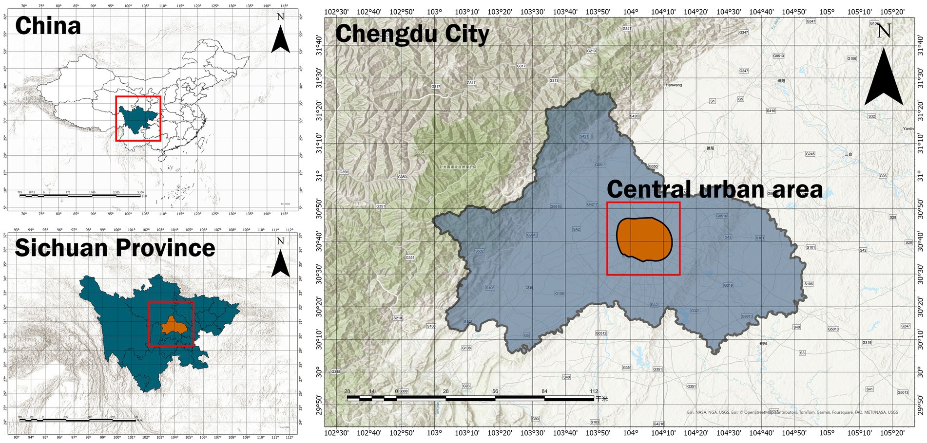
Figure 1. China map (left top), Sichuan Province map (left bottom), and Chengdu map (right).

3 Data and methods

3.1 Data collection and processing

The core data for this study primarily comes from remote sensing imagery, urban geographic information, and Geographic Information System (GIS) datasets. The study area is the central urban district of Chengdu, with its boundaries defined by the Chengdu Ring Expressway. To assess Urban Green Space demand, the following data were collected: 2024 Land Surface Temperature (LST) TIFF data, 2022 carbon dioxide concentration TIFF data, 2024 population density TIFF data, the boundary data of the central urban area of Chengdu, and the 2024 urban green space Shapefile (SHP) data for the central urban area of Chengdu (Figure 2). All data were uniformly processed in space to ensure consistency in the coordinate system and resolution across datasets, thus providing a solid data foundation for subsequent analysis.

Figure 2

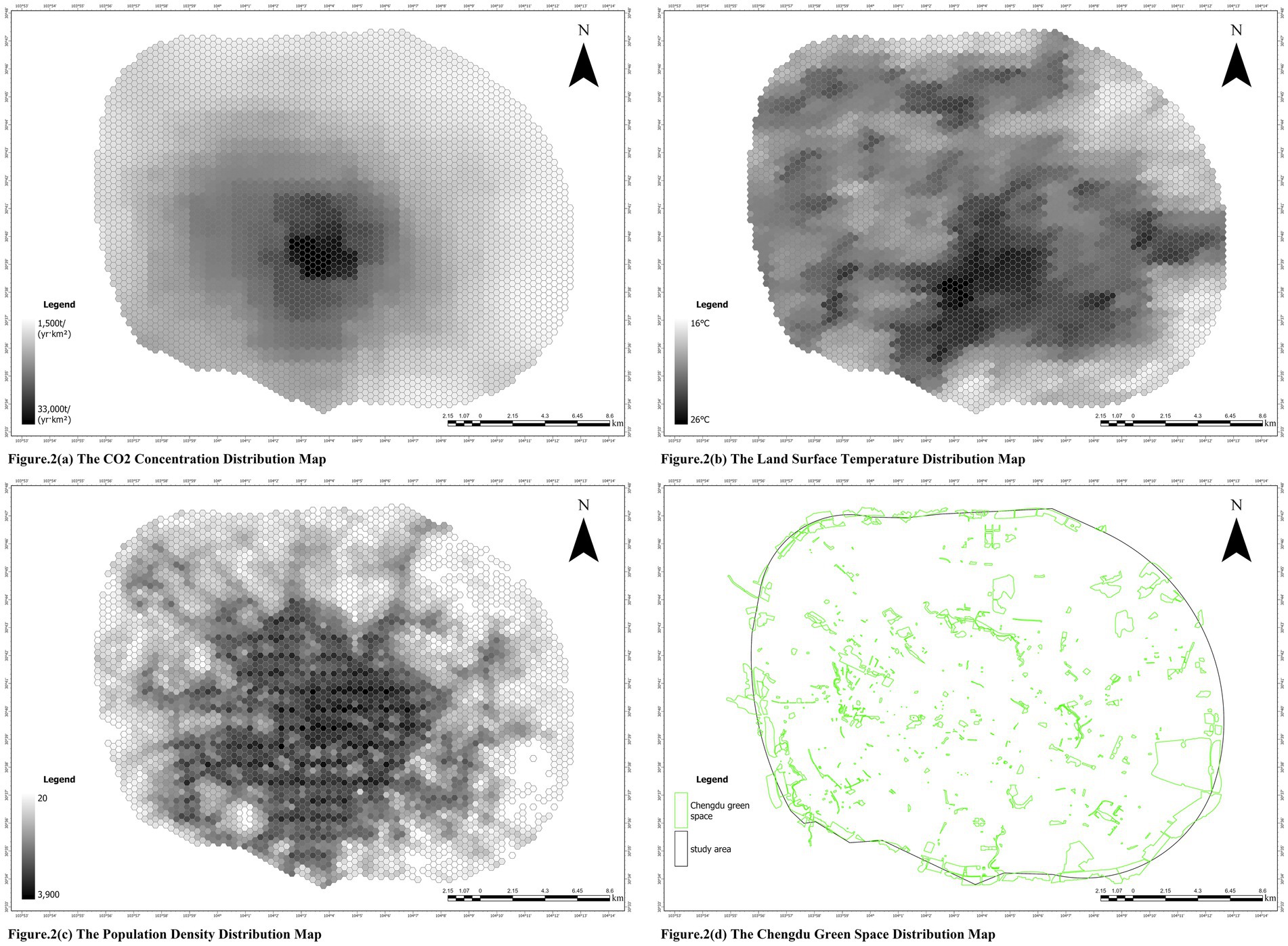
Figure 2. (a) The CO2 concentration distribution map. (b) The land surface temperature distribution map. (c) The population density distribution map. (d) The Chengdu green space distribution map.

In this study, the boundary of the central urban area of Chengdu is defined according to the “Chengdu Urban Master Plan (2011–2020)” and refers to the area enclosed by the Chengdu Ring Expressway (Qiao et al., 2024). The Land Surface Temperature (LST) data were obtained through inversion techniques from Landsat remote sensing imagery, and were corrected using standard atmospheric and surface meteorological data, ensuring high accuracy and extensive spatial coverage. This data effectively reveals the distribution characteristics of the urban heat island effect (Vaishnavi et al., 2024). The carbon dioxide concentration data were sourced from the ODIAC dataset provided by the Center for Global Environmental Research, which serves as an important indicator of urban carbon sequestration demand and ecological environmental quality. This data is crucial for air quality and climate change analysis (Xie et al., 2023). The population density data were obtained from the World Pop website, which provides high-resolution global population distribution information and offers detailed data support for understanding the spatial distribution of social demand for urban green space. Additionally, the urban green space data for the central urban area of Chengdu is provided in Shapefile format and sourced from OpenStreetMap public data. This dataset includes spatial information for all known green spaces and parks and serves as the foundational data for conducting green space demand assessments.

In the data preprocessing stage, all datasets underwent sequential refinement to ensure spatial integrity and analytical consistency, beginning with strict coordinate registration for geographic alignment, followed by comprehensive missing value imputation using k-nearest neighbors interpolation, and concluding with format standardization to homogenize data structures. To specifically address noise sensitivity inherent in unsupervised learning, we implemented robust outlier detection via the Interquartile Range (IQR) method (±1.5 × IQR threshold), flagging extreme values for winsorization, coupled with non-parametric scaling through RobustScaler (scikit-learn implementation), which centers data by the median and scales by interquartile range to diminish outlier influence. These targeted preprocessing procedures collectively enhanced the noise robustness of subsequent autoencoder training. Finally, spatial overlay and analytical operations were performed in GIS to derive per-grid green space demand indices, yielding refined datasets for segmented feature extraction.

These preprocessing enhancements substantially fortified the noise robustness of subsequent autoencoder training. Following data sanitization, GIS-based spatial overlay and analytical operations were applied to derive per-grid green space demand indices. The resultant refined datasets provided a reliable foundation for segmented feature extraction and autoencoder-based latent space learning.

3.2 Overview of the methodology

This study proposes an autoencoder-based framework for assessing Urban Green Space demand (Figure 3), which comprehensively considers both social and ecological dimensions. First, the study area is divided into 200-m side-length hexagonal grids. The Gaussian two-step moving search method is then used to calculate social demand based on green space accessibility and ecological demand based on heat island effect mitigating capacity and carbon sequestration capacity. Next, an autoencoder is employed to perform feature learning on the three types of demand data, extracting green space demand features and other relevant characteristics from the encoded vectors in the latent space. Finally, the obtained latent features are subjected to k-means++ clustering for dimensionality reduction. Through the convergence of the trained model, the final differences in Urban Green Space demand across regions are determined, providing a scientific basis for the optimized allocation of urban green space resources.

Figure 3

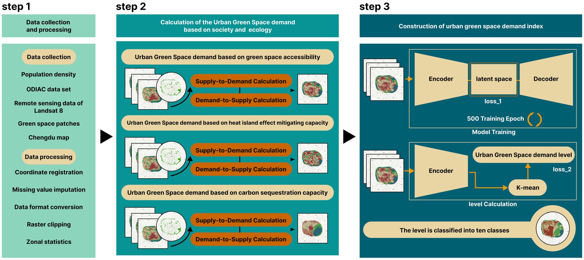
Figure 3. Research process flowchart.

3.3 Multidimensional urban green space demand calculation

In this phase, the city is first divided into hexagonal grid cells with a side length of 200 m, which serve as the basic units for spatial analysis. Based on these grids, this study innovatively applies the Gaussian two-step moving search method (2SFCA) to calculate the Urban Green Space demand in three dimensions: demand based on green space accessibility, demand based on heat island effect mitigating capacity, and demand based on carbon sequestration capacity.

3.3.1 Green space demand based on accessibility

This study uses accessibility as a core measure of urban social demand, aiming to analyze the responsiveness of green space resources in meeting residents’ rights to live and their social welfare needs. Based on the urban spatial justice theoretical framework, high-density residential areas experience a significant increase in population aggregation and ecological service demand intensity, making the mismatch between green space supply and demand more pronounced. Therefore, accessibility is prioritized as the parameter for demand-side evaluation (Czesak and Różycka-Czas, 2025). In terms of spatial analysis methodology, an improved two-step floating catchment area (2SFCA) method is applied, with a 1,000-m service radius threshold for measuring accessibility. This threshold is based on the “15-min living circle” spatial scale standard outlined in the “Urban Residential Area Planning and Design Standards,” which aligns with residents’ daily recreational behaviors and effectively reflects the spatiotemporal efficiency of urban green space service coverage. This method uses a dual-search mechanism to simultaneously consider the spatial matching relationship between the supply side (green space service capacity) and the demand side (population density), accurately identifying areas with high demand but low supply (Long et al., 2024).

3.3.2 Green space demand based on heat island effect mitigating capacity

The urban heat island effect refers to the phenomenon where urban areas experience elevated temperatures due to the abundance of artificial facilities and dense buildings (Kim and Brown, 2021). To mitigate this effect, increasing green space coverage is critical for reducing urban temperatures. This study further evaluates the impact of the heat island effect on green space demand by analyzing the relationship between land surface temperature changes and green space distribution. In terms of spatial analysis methodology, we used an improved two-step floating catchment area (2SFCA) method to quantify green space demand and introduced a Gaussian decay function to replace the traditional binary method. This continuous decay model better aligns with the spatial decay pattern of heat environment improvement effects (Xue et al., 2023). The core advantage of the two-step floating catchment area method lies in its bidirectional supply–demand matching mechanism, which not only considers the supply capacity of green space resources (such as patch area and vegetation coverage) but also integrates the spatial demand weight of heat island intensity areas. We set a 500-m service radius threshold, which was selected based on dual validation: on one hand, behavioral geography studies show that when walking distances exceed 500 m, the likelihood of residents choosing to enter green spaces for cooling drops significantly by 63.7%; on the other hand, the negative correlation between land surface temperature (LST) and green space patches peaks at the 500-m scale (r = −0.71, p < 0.01), indicating that this radius effectively captures the boundary effect of green space on microclimate regulation (Zhang et al., 2025; Wang et al., 2019).

3.3.3 Green space demand based on carbon sequestration capacity

The carbon sequestration function is one of the key ecological functions of green spaces in addressing climate change. By calculating the potential carbon sequestration capacity of green spaces in different regions, this study assesses the demand for green space in terms of carbon dioxide absorption and the reduction of greenhouse gas emissions. Previous studies have shown that urban green spaces’ carbon dioxide absorption is mainly concentrated within a 10-km range. Therefore, this study uses a 10-km radius for green space supply and demand matching, constructing a supply capacity table for each green space based on this radius (Gao et al., 2024; Xu et al., 2023). Given the typical demand–supply relationship between carbon dioxide absorption demand and the green space absorption radius, the study employs the two-step floating catchment area (2SFCA) method to calculate green space demand based on carbon sequestration capacity, clearly reflecting the impact of carbon dioxide concentration on urban green space demand in the central urban area of Chengdu.

3.3.4 Gaussian two-step floating catchment area (Ga2SFCA)

The Gaussian Two-Step Floating Catchment Area (Ga2SFCA) is a method used to analyze the spatial accessibility of public service facilities. By incorporating a Gaussian function to address the distance decay issue, this method more accurately measures the accessibility of facilities. Below are the formula and parameter explanations:

$R_j=\frac{S_j}{{\sum }_{k\in \{d_{\mathit{kj}}\le d_0\}}{P}_k·G(d_{\mathit{kj}},d_0)}$

$A_i={\sum }_{j\in \{d_{\mathit{kj}}\le d_0\}}{R}_j$

• i: Demand point, such as a residential area or street;

• j: Supply point, such as a hospital, green space, or other facilities;

• d_kj: The distance between demand point i and supply point j;

• d0: Search radius threshold, used to define the spatial scope of the supply and demand points;

• P_k: The demand population at demand point k;

• S_j: The service capacity of supply point j, such as the area of green space or the number of hospital beds;

• R_j: The supply–demand ratio at supply point j, i.e., the ratio of service capacity to the potential demand population;

• A_i: The accessibility of demand point i, representing the degree to which the point can access the supply facility.

G (d_kj, d0): Gaussian decay function, used to account for the impact of distance decay on accessibility. The formula is:

$G(d_{\mathit{kj}},d_0)=\frac{e^{-\frac{1}{2}{\left(\frac{d_{\mathit{kj}}}{d_0}\right)}^2}}{1-e^{-\frac{1}{2}}}$

e refers to the base of the natural logarithm.

3.4 Extraction of nonlinear features using autoencoders

Autoencoder (AE) is an unsupervised learning algorithm designed to learn effective representations of data. It is widely used in tasks such as dimensionality reduction and feature extraction, as shown in Figure 4. An autoencoder consists of two parts: an encoder and a decoder. The encoder maps the input data to a low-dimensional latent space representation, while the decoder attempts to reconstruct the original input from this low-dimensional representation. The goal of an autoencoder is to minimize the reconstruction error, which is the difference between the input and the output, thereby forcing the model to learn the most important features of the data (Liu et al., 2018).

Figure 4

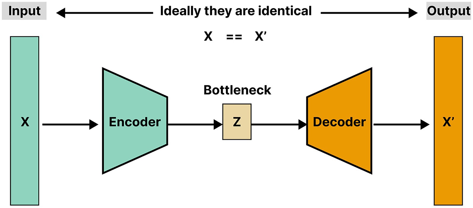
Figure 4. Classic autoencoder architecture.

During the training process, the autoencoder adjusts its parameters using backpropagation and gradient descent optimization algorithms, gradually improving its reconstruction ability and feature extraction performance. This study proposes a framework that combines the autoencoder with the k-means++ clustering algorithm, aimed at evaluating the regional differences in Urban Green Space demand. This framework effectively captures the complex internal structure of urban green space demand. The data for this study mainly include remote sensing imagery, urban geographic data, and GIS datasets. After preprocessing, three key indicators—heat island effect mitigating capacity (HIEMC), carbon sequestration capacity (CEC), and green space accessibility (GSA)—were extracted, normalized, and stored in CSV files for subsequent analysis.

In the clustering analysis, this study employs the K-means++ clustering algorithm to cluster the latent features extracted by the autoencoder. The clustering process involves sorting and reallocating the cluster center means, ultimately dividing urban areas into different levels of green space demand. Specifically, a custom autoencoder model was designed, consisting of an encoder, an auxiliary classification branch, and a decoder (Figure 5). The encoder uses a five-layer fully connected network to map the input data to an 8-dimensional bottleneck layer to obtain a global low-dimensional latent representation.

Figure 5

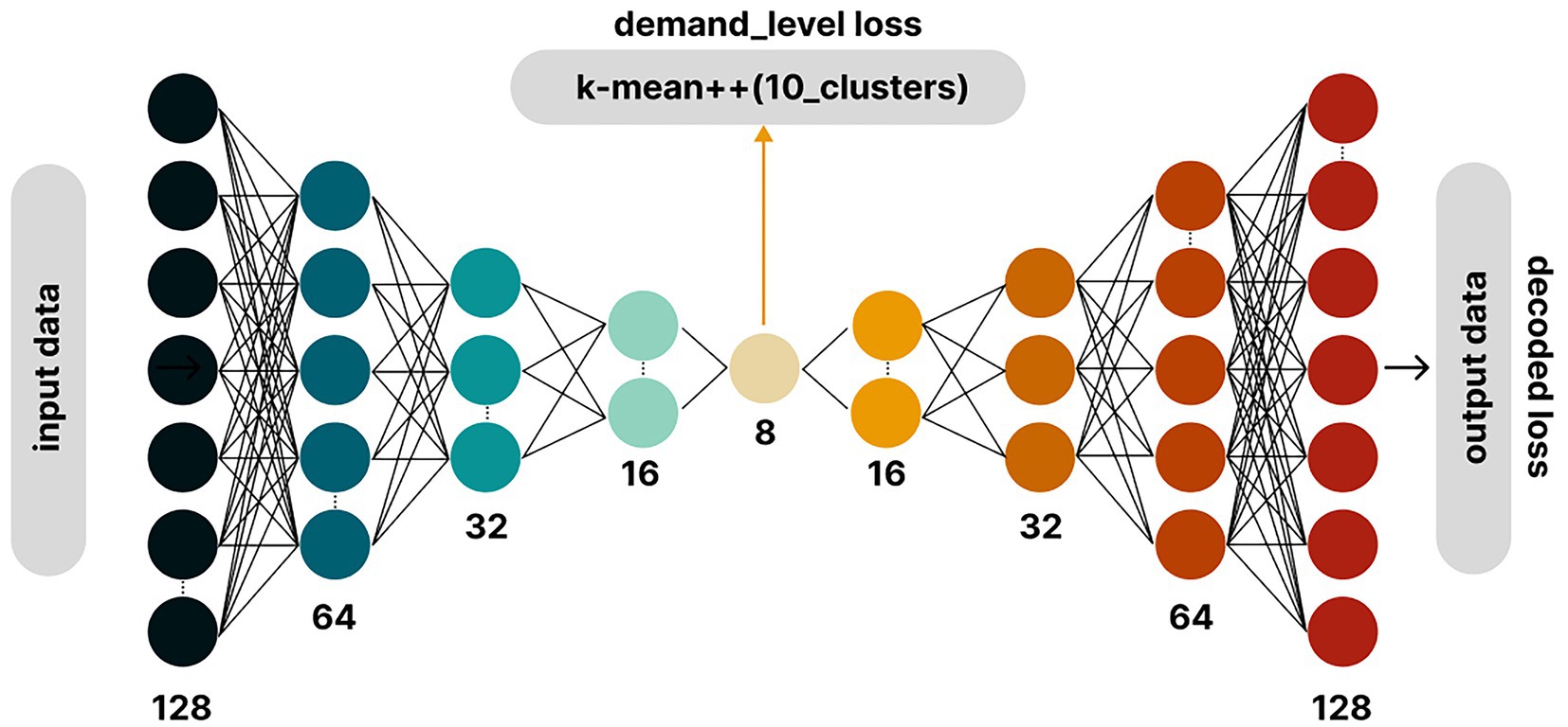
Figure 5. The model structure includes the autoencoder layers and the k-means++ clustering branch.

To achieve clustering of the latent features, an auxiliary classification branch was introduced based on the bottleneck layer. This branch uses the improved k-means++ algorithm to cluster the 8 latent features extracted by the autoencoder, ultimately resulting in 10 different levels of urban green space demand. During training, the reconstruction task is optimized using the mean squared error (MSE) loss function, while the classification task is optimized using the k-means++ algorithm.

3.4.1 Extraction of latent features from multidimensional data using autoencoders

In this study, the extraction of latent features is accomplished through the encoder part of the autoencoder model. First, the input data is standardized to ensure that the mean of each feature is zero and the variance is one. Standardization eliminates the differences in the scale of different features, enabling the model to learn better during the training process and preventing certain features from disproportionately affecting the model due to scale issues. The standardized data is then fed into the encoder part of the autoencoder, where it undergoes progressive mapping through multiple fully connected layers, ultimately compressing the data from high-dimensional space to a low-dimensional latent space (Figure 6).

Figure 6

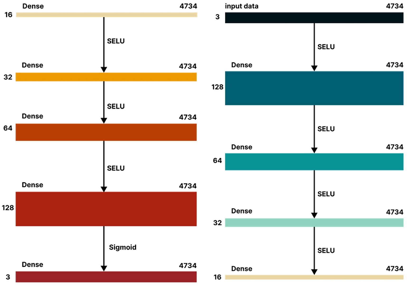
Figure 6. The autoencoder architecture, with the encoder on the left and the decoder on the right.

The encoder part of the autoencoder consists of several fully connected layers, with each layer progressively compressing the data through different numbers of neurons. Specifically, the first layer of the encoder has 128 neurons, the second layer has 64 neurons, the third layer has 32 neurons, the fourth layer has 16 neurons, and finally, the bottleneck layer (latent layer) compresses the data into an 8-dimensional latent representation. This 8-dimensional latent layer captures the key information from the input data and is the most representative part of the entire autoencoder. Through this compression, we not only reduce the dimensionality of the data but also remove redundant information, allowing the model to effectively retain the main features of the data.

In this process, we specifically chose SELU (Scaled Exponential Linear Units) as the activation function. SELU is an activation function that has been widely used in deep neural networks in recent years, featuring self-normalizing properties. Compared to traditional activation functions such as ReLU and Sigmoid, SELU can effectively avoid the vanishing gradient problem in deep neural networks and accelerate the convergence speed of the model. The activation formula for SELU is as follows:

$\mathit{\text{SELU}}\left(x\right)=\lambda \{\begin{array}{cc}x& \mathit{\text{if}}x>0\\ \alpha (e^x-1)& \mathit{\text{if}}x\le 0\end{array}$

Where λ and α are hyperparameters, typically set to λ = 1.0507 and α = 1.6733. The piecewise linear function in this formula ensures that SELU behaves as a linear function in the positive region and as an exponentially growing function in the negative region, thereby stabilizing the activation values within a certain range. Unlike the traditional ReLU function, SELU not only avoids the dead neuron problem but also maintains the variance of signals in the network, improving stability during the training process.

One of the key advantages of SELU is its self-normalizing property. It can automatically adjust the output of neurons in the network, maintaining the distribution of activation values in deep networks. Traditional activation functions, such as ReLU, are prone to gradient vanishing or explosion issues, especially in deep networks, leading to instability during training. However, SELU ensures that activation values maintain relatively consistent variance during propagation through each layer, which promotes effective gradient propagation and improves the training efficiency of deep neural networks.

By using the SELU activation function in each layer, we can ensure that the autoencoder is more stable during training and converges faster. Specifically, the activation output of each layer is processed through the SELU function, ensuring that the signals in the network maintain an appropriate distribution and avoiding potential issues with gradient vanishing or explosion during training. This not only enhances the stability of the training process but also accelerates it, allowing the autoencoder to effectively learn the deep features within the data.

During the training process, the Mean Squared Error (MSE) is used as the loss function, with the goal of minimizing the difference between the original input data and the reconstructed data. The formula for calculating the MSE is as follows:

$\mathit{MSE}=\frac{1}{n}{\sum }_{i=1}^n{(x_i-\widehat{x_i})}^2$

where $\widehat{x_i}$ is the reconstructed data from the model, x_i is the original input data, and n is the number of samples. By minimizing this loss function, the model can continuously optimize its parameters during training, enabling a more accurate representation of the input data in the latent space.

During training, the Adam optimizer is used, with a learning rate set to 0.0001. After training for 500 epochs, the model can extract low-dimensional latent features from the standardized data. The latent features extracted by the encoder represent a low-dimensional depiction of the data, containing key information from the original data while removing redundant dimensions, thus providing concise and representative input for subsequent analysis (Bhattacharjee et al., 2024; Zhang et al., 2024; Rochmawati et al., 2021; Hazra et al., 2020).

Finally, after the training is complete, the latent features extracted by the encoder will be saved in a new data table, along with the ID of each sample, for future clustering analysis or other data analysis tasks. Through this process, we have extracted low-dimensional, information-rich latent features from high-dimensional data, providing strong data support for the subsequent clustering analysis.

In summary, the reason for selecting SELU as the activation function lies in its self-normalizing properties, which effectively avoid the vanishing gradient problem in deep neural networks and accelerate the convergence process of the network. Additionally, the use of SELU in each layer ensures that the model can converge stably during training, improving training efficiency. Moreover, by extracting latent features through the autoencoder, we have successfully mapped high-dimensional data to a low-dimensional latent space, thus providing a more concise and efficient representation for subsequent analysis (Sakketou and Ampazis, 2019; Pratama and Kang, 2020; Lu et al., 2023).

The specific autoencoder parameters are shown in Table 1.

Table 1

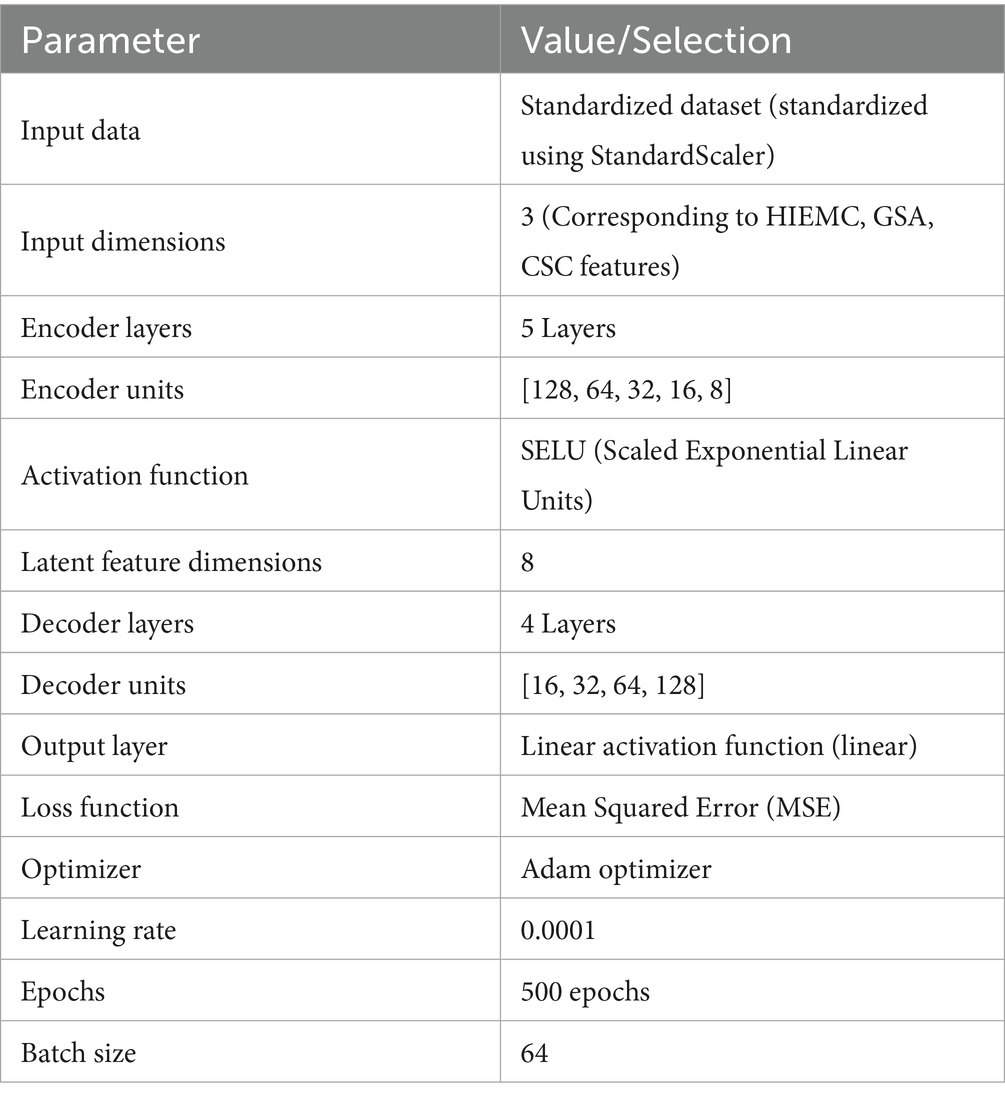
Table 1. Autoencoder parameter table.

3.4.2 Clustering of latent features using the K-means++ algorithm

In this study, the clustering process uses the K-means++ algorithm, aimed at effectively clustering the latent features extracted by the autoencoder. K-means++ is an improvement of the classic K-means algorithm, primarily designed to enhance the stability and quality of clustering results by optimizing the selection of initial cluster centers. Compared to the traditional K-means algorithm, K-means++ reduces the negative impact of uneven initialization of cluster centers by using a more intelligent initialization step, thus avoiding the issue of getting trapped in local minima.

The initialization steps of K-means++ can be summarized as follows:

Selecting the first cluster center: Randomly choose a data point from all the data points as the first cluster center.

Selecting subsequent cluster centers: For each remaining data point, calculate the Euclidean distance from the point to the already selected cluster centers, and select the next cluster center based on the squared distance to the total distance ratio. Specifically, the probability of selecting a point as a cluster center is proportional to the squared distance from it to the current cluster centers.

Repeating step 2 until the required number of cluster centers (in this study, 10 cluster centers) are chosen (Cohn and Holm, 2021).

This initialization method ensures that the initial cluster centers are spaced apart, which helps the clustering process converge more effectively.

In this study, the K-means++ algorithm was applied to cluster the 8-dimensional latent features extracted by the autoencoder. First, the data were standardized to ensure that each feature had a zero mean and unit variance, which helps reduce the impact of scale differences between features on the clustering results. Then, the K-means algorithm was applied with the “init” = ‘k-means++’ parameter to cluster the data using the K-means++ initialization method. In the code implementation, the “kmeans.fit_predict(data_scaled)” function was used to cluster the standardized data and return the cluster labels for each sample.

The key advantage of the K-means++ algorithm is its ability to reduce the dependence of clustering results on the initial conditions by optimizing the selection of initial cluster centers, thus improving the stability and accuracy of clustering. Through clustering, we were able to divide the latent features into 10 different clusters, with each cluster representing similar data points in the latent feature space.

After the K-means++ clustering was completed, to further evaluate the clustering results, we calculated the Euclidean norm (L2 norm) of each cluster center, which represents the distance from the cluster center to the origin. The formula for calculating the Euclidean norm is as follows:

$\mid c_i\mid =\sqrt{{\sum }_{j=1}^n{\left(c_{\mathit{ij}}\right)}^2}$

Where c_i represents the i-th cluster center, c_ij represents the coordinate of the i-th cluster center in the j-th dimension, and n is the dimensionality of the data. In this study, the dimensionality of the cluster centers is 8, so the Euclidean norm calculates the distance of each cluster center from the origin.

Next, using the calculated Euclidean norms, we sorted the cluster centers. Cluster centers that are closer to the origin were assigned to smaller ranks, while those further from the origin were assigned to larger ranks. Through this ranking, we were able to assign a rank to each cluster and assess the nature of the clusters based on the relative positions of the cluster centers.

Finally, the clustering labels and rank information were stored in a new Excel file for subsequent analysis and visualization. Through K-means++ clustering and the calculation of Euclidean norms, we gained deeper insights into the latent structure of the data and provided a solid foundation for subsequent regional analysis.

3.4.3 Result visualization

The result of the visualization process in this study was based on GIS PRO software. First, the K-means++ clustering results obtained in the study were imported into the GIS PRO environment. Building on this, the clustering results were integrated with the attribute table of the cellular network in the study area, further combining geographic spatial data with clustering information. This process not only effectively visualized the data in a geospatial context but also enhanced the connection between clustering analysis and the actual regional attributes, providing more intuitive support for the visualization of the research results. Finally, combining the attributes of the cellular network, the clustering results for the study area were clearly displayed, providing important visual support for subsequent spatial analysis and decision-making.

4 Results

4.1 Model training results

In this study, feature extraction of urban green space demand data was performed using an autoencoder model. The training process used standardized data (including GSA, CEC, and HIEMC features) and employed the Adam optimizer and SELU activation function. The training ran for a total of 100 epochs, with each epoch utilizing a batch size of 32 samples.

4.1.1 Reconstruction error analysis

The objective of the autoencoder model is to minimize the mean squared error (MSE) between the input data and the reconstructed data. Upon completion of training, the model successfully compressed the input data from three-dimensional space to an 8-dimensional latent space, while keeping the reconstruction error at a low level. Specifically, the MSE stabilized at approximately 4.71e-05 during the final stages of training, indicating that the model effectively retained key information of the data during compression and reconstruction.

4.1.2 Latent feature extraction

Using the trained autoencoder model, we extracted 8 latent features from the data. These features effectively represent the primary variations in the original data and were used for subsequent clustering analysis. The extraction of latent features not only reduced the dimensionality but also enhanced the model’s ability to capture the intrinsic structure of the data.

4.1.3 Clustering results

Based on the extracted latent features, the K-means++ clustering algorithm was used to divide the data into 10 clusters. The Euclidean norm (L2 norm) of each cluster center was calculated and sorted in ascending order to determine the relative importance rank of each cluster. Using this method, we were able to identify differences in green space demand across different regions. The potential feature values for each clustering level are shown in Table 2.

Table 2

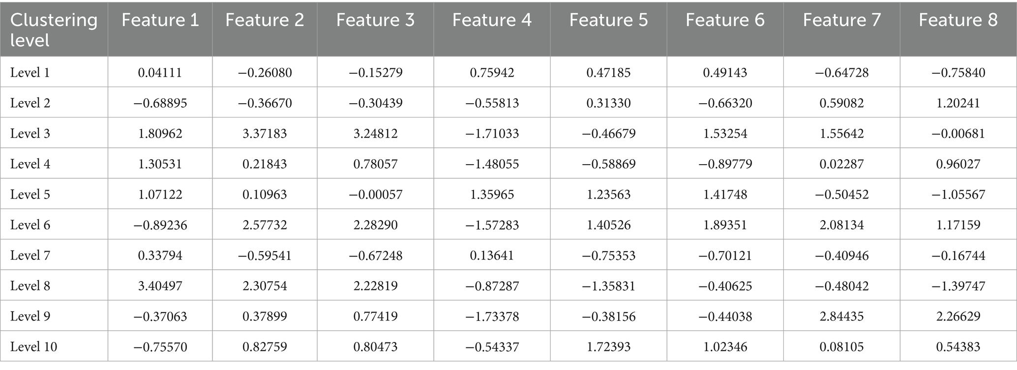
Table 2. The potential feature values of the cluster centroid.

Overall, the autoencoder model successfully extracted representative latent features from the original data and provided effective input for clustering analysis. The low reconstruction error during the training process indicates that the model performed well in data compression and reconstruction, and the subsequent clustering results further validate this.

4.2 Regional distribution of urban green space demand

After multiple rounds of training, we have derived the final regional distribution map of Urban Green Space demand. This series of maps illustrates the urban green space demand distribution in the central urban area of Chengdu, based on various environmental and social factors. Each map demonstrates how green space demand is influenced by specific factors, such as carbon sequestration, heat island effect mitigation, and accessibility. Below is a detailed analysis of each image and the fundamental patterns they reflect.

4.2.1 Green space demand based on carbon sequestration

The first map (Figure 7a) shows the distribution of urban green space demand based on carbon sequestration capacity (CSC). The color gradient indicates that demand is concentrated in areas with higher carbon dioxide emissions, typically located in industrial or densely populated regions. These areas with higher demand (darker regions) represent locations that need to counteract the negative environmental impacts of increased carbon dioxide concentrations through carbon sinks. Carbon sequestration demand is primarily concentrated in the city center and near major transportation hubs, where both population density and carbon dioxide emissions are higher.

Figure 7

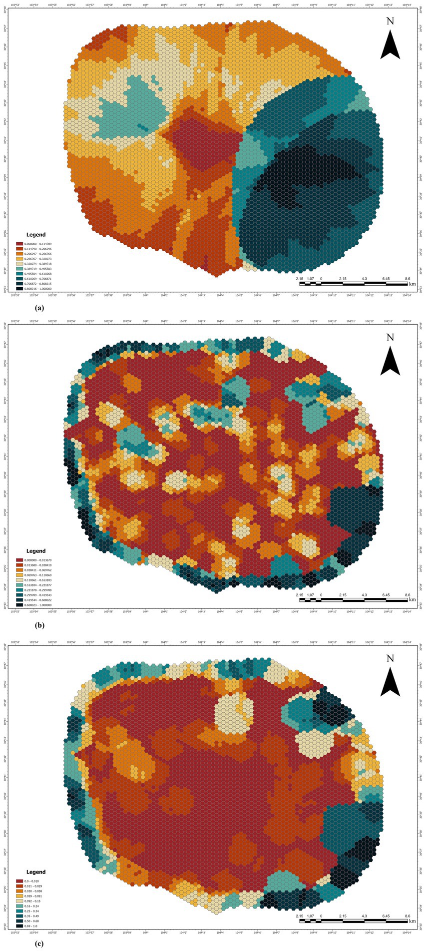
Figure 7. (a) Carbon sequestration capacity distribution. (b) Heat island effect mitigating capacity distribution. (c) Green space accessibility distribution.

This distribution suggests that these areas require special attention to green space supply in order to mitigate the negative environmental impacts of urbanization. The carbon sequestration capacity of green spaces in these areas can be an important strategy for reducing the urban carbon footprint, improving air quality, and contributing to climate change mitigation.

4.2.2 Green space demand based on heat island effect mitigation

The second map (Figure 7b) reflects the green space demand based on heat island effect mitigating capacity (HIEMC). Areas with strong heat island effects are shown in red and orange, which are typically high-heat urban areas with higher land surface temperatures (LST). This phenomenon is common in urban areas covered by impervious surfaces such as concrete and asphalt, which absorb and retain heat. This pattern is consistent with the widespread phenomenon of urban heat island effects, which intensify local temperature variations within cities.

Regions with more severe heat island effects require a large amount of green space to help cool the area and mitigate the urban heat effect. Analysis shows that the outskirts of the city (where urban sprawl is more noticeable) may also face more significant heat stress issues, further highlighting the necessity for effective urban green space planning to restore thermal comfort for urban residents.

4.2.3 Green space demand based on accessibility

The third map (Figure 7c) presents the green space demand distribution based on green space accessibility (GSA), focusing on the accessibility of green spaces, particularly the population density and ease of access to green spaces. Regions with higher demand are shown in yellow and orange, indicating that residents in these areas may face difficulties accessing green spaces. High-demand areas with dense populations point to the urgent need to improve green space accessibility, which is crucial for the quality of life of residents. These areas may include urban slums or places with insufficient green space coverage.

Using accessibility as a measure effectively highlights regions that need spatial interventions to improve green space accessibility. The analysis suggests that urban planning should focus on improving the connectivity of green spaces, especially in densely populated areas, to ensure all residents have equal access to natural spaces, which contributes to physical and mental health.

4.2.4 Comprehensive green space demand distribution

The final map (Figure 8) integrates carbon sequestration capacity (CSC), heat island effect mitigating capacity (HIEMC), and green space accessibility (GSA) to create a comprehensive green space demand distribution map. This integrated map provides a multidimensional perspective on urban green space demand, combining spatial needs related to carbon capture, temperature regulation, and accessibility. The most urgent demand areas (darker regions) are those with high carbon emissions, intense heat island effects, and poor green space accessibility.

Figure 8

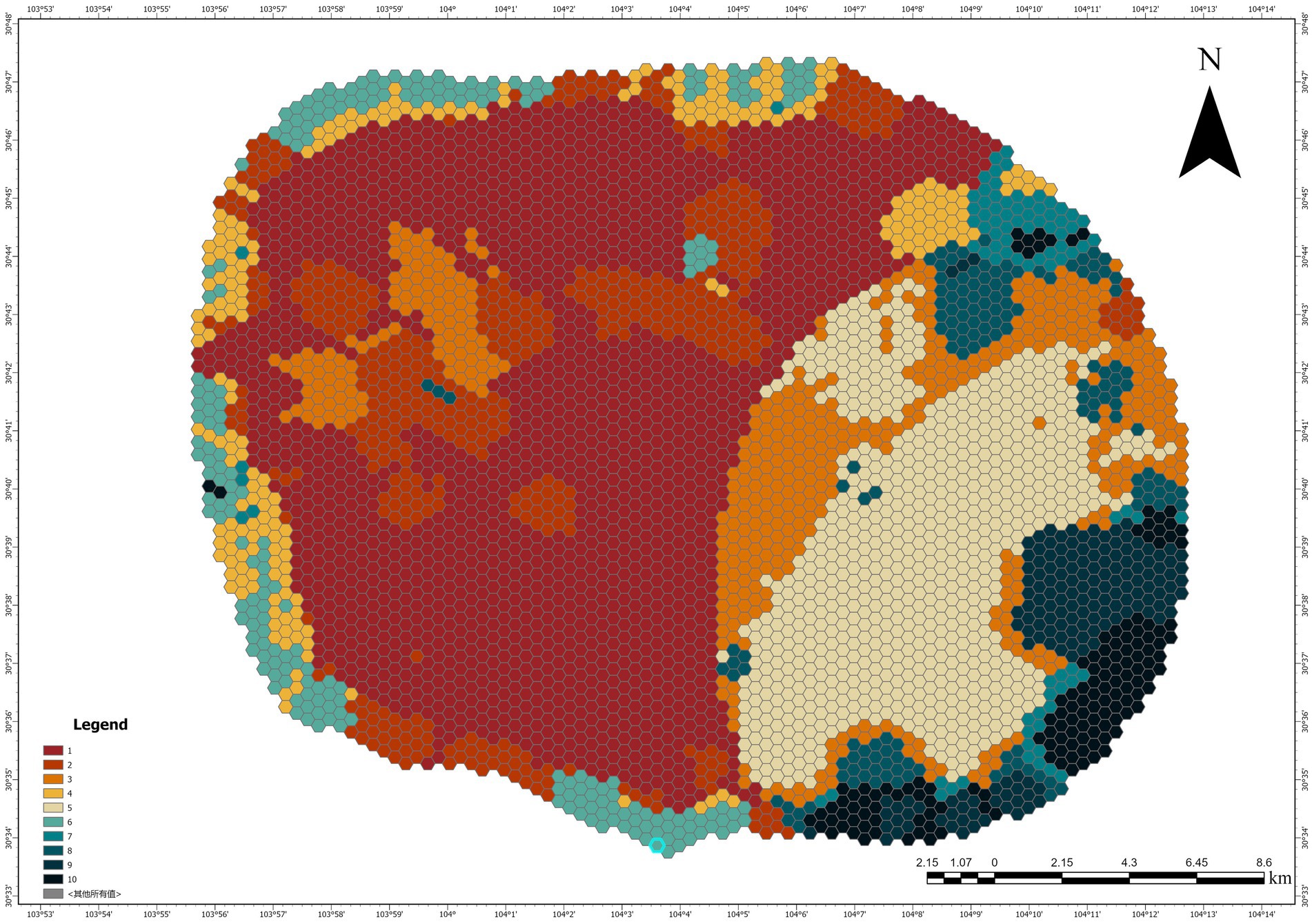
Figure 8. Regional variations distribution in urban green space demand.

The results show that the areas with the most urgent demand tend to be densely populated urban areas and transportation hubs, where there is a high demand for carbon sequestration capacity and a significant urban heat island effect. Furthermore, these areas face high population pressures on green space, and the existing fragmented green spaces struggle to meet these needs.

Analyzing this comprehensive map is crucial for urban planners and decision-makers, as it helps prioritize areas that most require green space interventions. For example, areas with high carbon emissions, severe temperature increases, and poor green coverage, especially in central and suburban zones, should be the focus of sustainable urban greening plans. Providing green spaces in these areas can not only reduce carbon emissions but also mitigate urban heat island effects and improve living conditions for urban residents.

4.3 Summary

These visual analyses provide valuable insights into the distribution of green space demand across different environmental and social dimensions. The maps highlight areas with low carbon emissions, severe heat island effects, and poor accessibility that need particular attention to green space provision. By focusing on these areas, urban planners can create green spaces that contribute to environmental sustainability while enhancing the quality of life for urban residents. This integrated approach, combining ecological, social, and accessibility factors, is essential for the sustainable development and resilience of Chengdu’s urban landscape.

5 Discussion

5.1 Comparison of PCA and autoencoder performance

Principal component analysis (PCA) is a classical method used for data dimensionality reduction and feature index extraction, widely applied in many studies. This study aims to explore the differences between the PCA method and an autoencoder model based on weakly supervised learning in terms of their ability to reduce data dimensions and extract feature indices. We analyzed the spatial distribution of Urban Green Space demand and the initial data reconstruction capabilities derived from both methods.

5.1.1 Logical connotations of autoencoder and principal component analysis

Both autoencoder (AE) and principal component analysis (PCA) are effective techniques for data dimensionality reduction, but their logical foundations and application contexts differ. PCA is a linear transformation-based dimensionality reduction method that finds the direction of maximum variance in the data by linearly combining the original data’s features. It extracts the most informative principal components by maximizing the variance of the data. The core idea behind PCA is to preserve the most important structural features of the data by maximizing its variance. PCA assumes that the data has a linear relationship, so its performance may be limited when dealing with nonlinear data.

In contrast, an autoencoder is a neural network-based nonlinear dimensionality reduction method. The autoencoder maps input data into a low-dimensional latent space through an encoder and reconstructs the original data through a decoder. The objective of an autoencoder is to minimize reconstruction error, thus learning the latent structure of the data. Unlike PCA’s linear assumption, the autoencoder can handle nonlinear relationships in the data, which makes it more expressive when dealing with complex, high-dimensional data. By optimizing its network architecture and training process, the autoencoder can extract richer and deeper features in the latent space compared to PCA.

5.1.2 Information retention and reconstruction error

To compare the effectiveness of the Urban Green Space demand obtained through dimensionality reduction by PCA and autoencoder models, we further explored the relationship between information retention and reconstruction error by calculating the inverse reconstruction capacity of both models. In the process, the three features in the original data were first subjected to principal component analysis (PCA), resulting in the following covariance matrix (Table 3):

Table 3

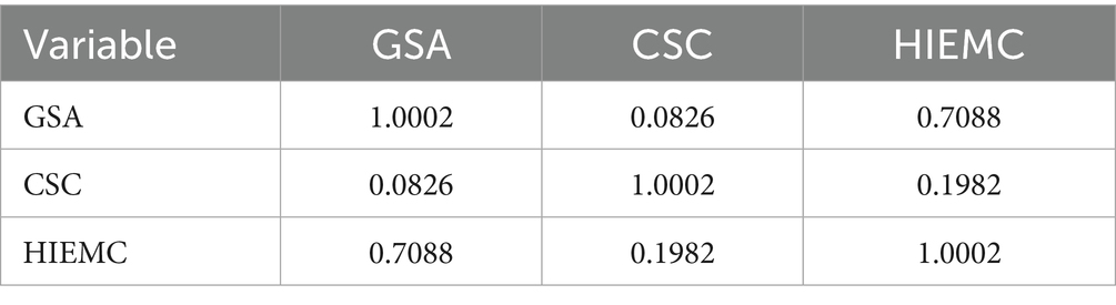
Table 3. Covariance matrix table.

From this, it can be observed that there is a strong positive correlation (0.7088) between heat island effect mitigating capacity (HIEMC) and green space accessibility (GSA), while the correlation between carbon sequestration capacity (CSC) and other variables is relatively weak. Based on this covariance matrix, the weight vectors of the principal components were further calculated, resulting in the following (Table 4):

Table 4

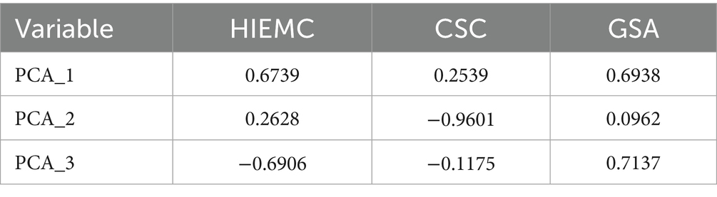
Table 4. Principal component weight vectors table.

The PCA results revealed the varying contributions of HIEMC, GSA, and CSC to the latent variance in the data. The first principal component (PCA_1) is primarily influenced by HIEMC and GSA, both contributing significantly and being positively correlated, indicating a strong relationship between these two variables. The second principal component (PCA_2) is mainly dominated by CSC, reflecting its independence relative to the other variables. In the third principal component (PCA_3), significant interactions between GSA and CSC are observed.

Next, we analyzed the proportion of variance explained by each principal component, with the following results: the first principal component explained 58.69% of the variance, the second principal component explained 31.92%, and the third principal component explained 9.39%. Overall, the first two principal components explained 90.61% of the variance, indicating that most of the data’s variance was effectively retained.

Regarding reconstruction error, when one principal component was retained, the reconstruction error (mean squared error, MSE) of the PCA model was 1.82e-02. When two principal components were retained, the reconstruction error decreased to 3.01e-03. In contrast, the autoencoder demonstrated exceptionally high performance on the same dataset, with a final average reconstruction error of 4.71e-05, significantly lower than the PCA model’s performance. This suggests that the autoencoder has a stronger advantage in preserving the complexity and nonlinear relationships in the data, enabling it to more accurately reconstruct the input data.

From this analysis, it is evident that while PCA effectively extracts key features and retains a large proportion of the variance in data dimensionality reduction, the autoencoder, through its nonlinear feature extraction mechanism, significantly enhances the accuracy of data reconstruction. This highlights its superior performance in extracting nonlinear features.

5.1.3 Statistical results of autoencoder and principal component analysis

First, to compare the performance of the two methods (autoencoder and PCA) in data dimensionality reduction in detail, we conducted a regional difference analysis of the Urban Green Space demand results obtained from both methods. The results are shown in two figures, with the Urban Green Space demand distributions obtained through dimensionality reduction by the autoencoder (Figure 9) and PCA (Figure 10), respectively. By comparing the results of these two methods, we can observe the differences in their performance when handling the linear and nonlinear features of the data.

Figure 9

Figure 9. Urban green space demand distribution based on autoencoder and urban green space.

Figure 10

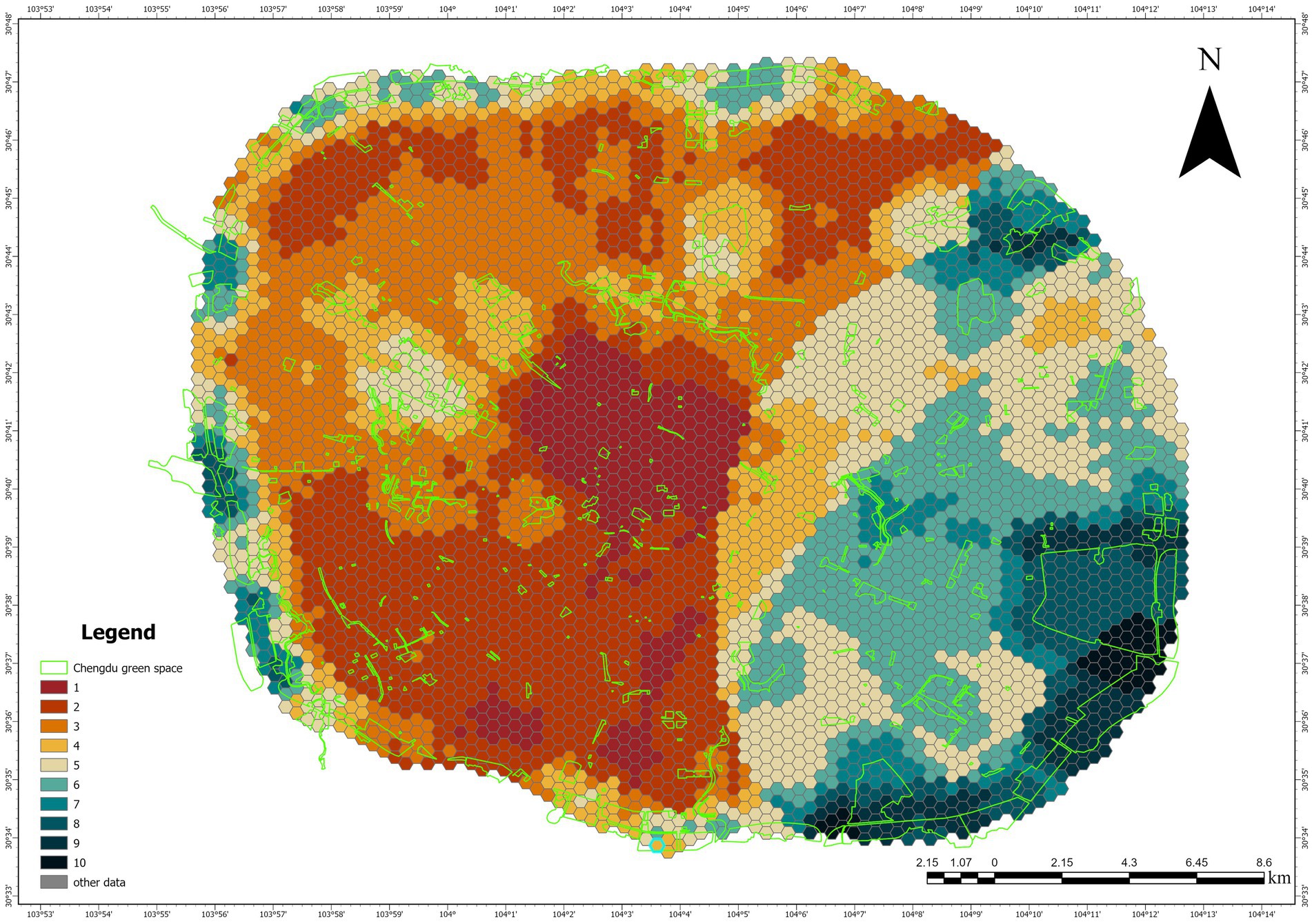
Figure 10. Urban green space demand distribution based on PCA and urban green space distribution.

As a linear dimensionality reduction method, PCA assumes that there are linear relationships between data features. In the right figure, PCA shows a relatively clear division after dimensionality reduction, but its performance also has certain limitations. Specifically, in some complex areas, PCA failed to effectively capture the nonlinear features of the data, leading to over-simplification or information loss in regions with subtle changes. This phenomenon indicates that PCA may not fully reflect the data structure when dealing with complex data that has nonlinear relationships.

In contrast, as a neural network-based nonlinear dimensionality reduction method, the autoencoder performs better at handling the nonlinear features of the data, as shown in the left figure. Although the image produced by the autoencoder does not have as obvious a distinction as that of PCA, it is better at capturing the detailed changes brought about by nonlinear relationships in the data. Particularly in regions with higher demand, the autoencoder retains more local variations and complex patterns, demonstrating its advantages in handling nonlinear data.

Overall, while the autoencoder may not show as clear a distinction as PCA in certain regions, it is more effective at preserving the latent structure of the data when handling complex nonlinear relationships, avoiding the simplification issues that PCA might encounter when dealing with nonlinear features. Therefore, the autoencoder can provide a more accurate and comprehensive feature representation when faced with nonlinear data.

Secondly, we performed a statistical analysis of the results obtained from both methods. According to the statistical results (Figure 11; Table 5), the autoencoder demonstrates a higher capability in data dimensionality reduction and feature extraction, especially in reflecting the multidimensional and complex characteristics of the data, where its advantages are more evident. First, the standard deviation of the autoencoder (2.6) is higher than that of PCA (2.1), indicating that the autoencoder can capture more variation and detail. The higher standard deviation reflects a more dispersed data distribution, with the autoencoder being better at presenting the volatility and diversity within the data. This high volatility allows the autoencoder to effectively preserve the data features of different regions in complex, multidimensional urban demand analysis, avoiding information loss.

Figure 11

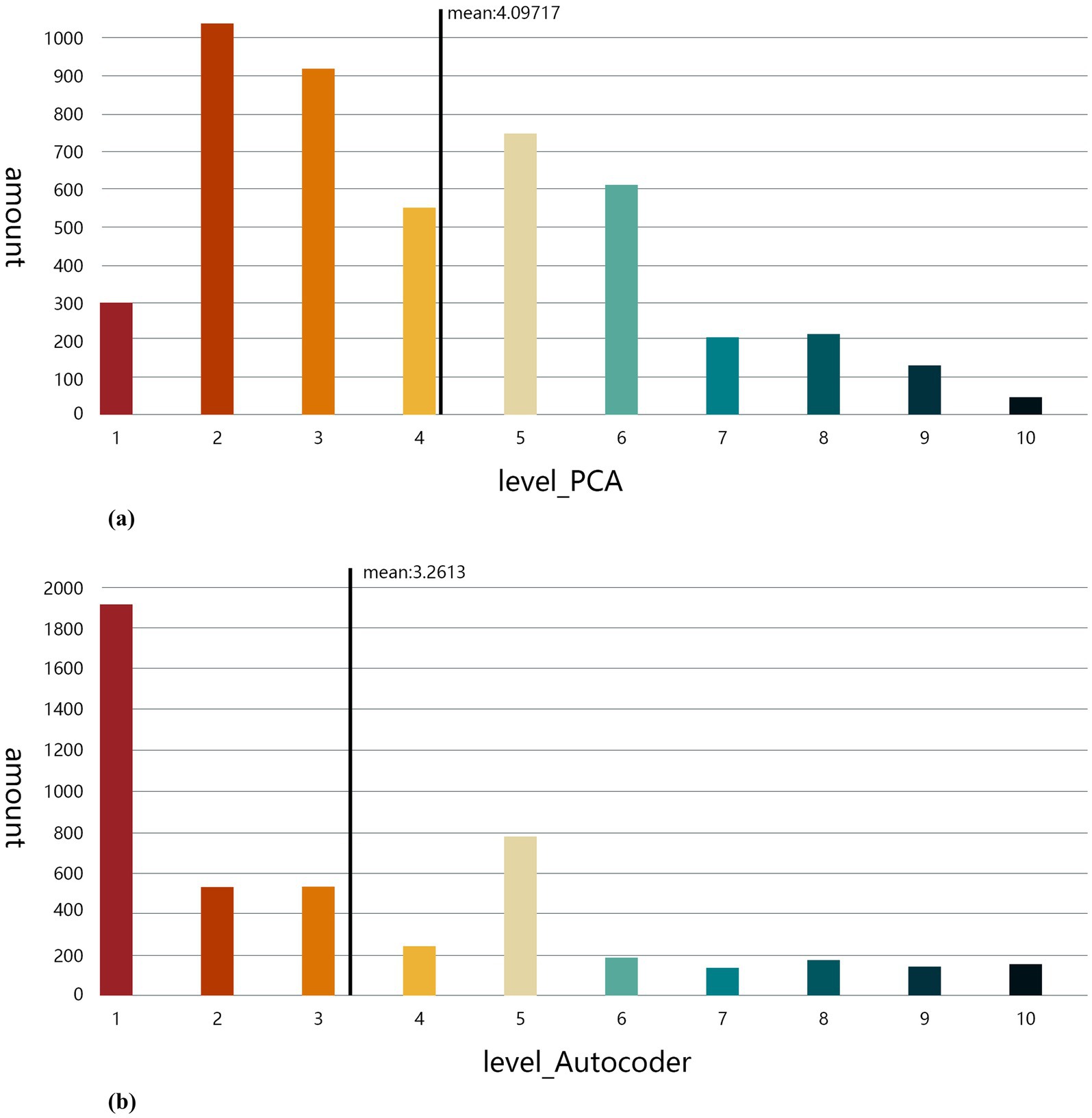
Figure 11. (a) Bar chart of PCA-based results. (b) Bar chart of autoencoder-based results.

Table 5

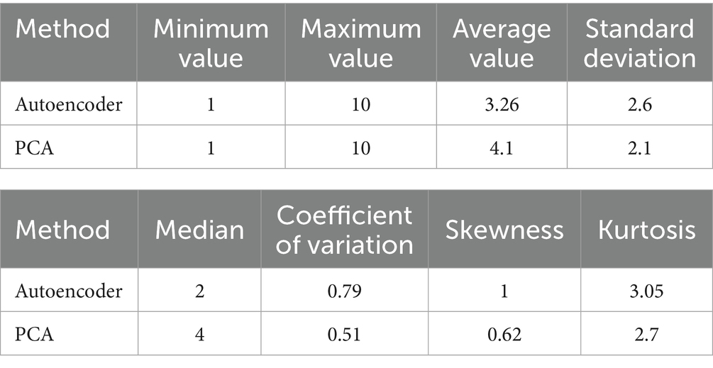
Table 5. Statistical results table.

Moreover, the coefficient of variation of the autoencoder (0.79) is higher than that of PCA (0.51), indicating that the autoencoder is more sensitive to the relative volatility of the data. The autoencoder maintains the data’s diversity during the dimensionality reduction process, capturing subtle differences in the data, particularly excelling at extracting nonlinear features.

In terms of skewness and kurtosis, the autoencoder also exhibits greater adaptability. The skewness (1) and kurtosis (3.05) of the autoencoder indicate significant asymmetry and concentration in the data distribution, reflecting the autoencoder’s ability to preserve local variations in the data after dimensionality reduction, particularly in regions with higher demand. This asymmetry demonstrates the autoencoder’s effectiveness in extracting nonlinear features from the data, making its dimensionality reduction results highly representative of the global structure of the data.

In contrast, PCA’s coefficient of variation (0.51) is lower, and its standard deviation (2.1) is relatively small, suggesting that PCA exhibits more stable characteristics when processing the data, with a more concentrated data distribution. PCA is particularly suitable for processing data with linear relationships, as it preserves the global structure of the data well and is effective at revealing overall trends. When dealing with data that shows clear linear relationships, PCA can effectively reduce dimensions while retaining key features, simplifying the data structure and extracting core information.

However, while PCA is very effective in handling data with strong linear relationships, it may be less effective when dealing with multidimensional, nonlinear, and complex data such as Urban Green Space demand. It may fail to capture nonlinear changes in the data effectively, leading to the loss of important information in complex demand analyses.

Therefore, in summary, the autoencoder provides more refined and accurate dimensionality reduction results when handling data with complex nonlinear relationships and multidimensional features. Its advantages are particularly evident in tasks such as Urban Green Space demand analysis. PCA, on the other hand, is more suitable for handling data with strong linear relationships and clear global structures, where it can effectively extract major features and reveal overall trends. Selecting the appropriate dimensionality reduction method based on the specific characteristics of the data and the analytical needs will help improve the accuracy and effectiveness of the analysis results.

5.2 Analysis of the feature extraction capability of the autoencoder

5.2.1 Relationship between clustering results and original data

In this study, the relationship between the clustering results and the original data was effectively revealed through the analysis of box plots. Two box plots illustrate the distribution of heat island effect mitigating capacity (HIEMC), carbon sequestration capacity (CSC), and green space accessibility (GSA) across different levels, from Level 1 to Level 10. These box plots provide valuable insights into the spatial distribution of each feature at various levels and reveal their relationship with Urban Green Space demand levels.

The first box plot (Figure 12a) displays the distribution of HIEMC, CSC, and GSA across all levels, showing the variations of each feature between levels. HIEMC typically represents the heat intensity in urban areas. As the demand level increases, the variation in HIEMC significantly increases, especially in high-demand areas where the fluctuations in HIEMC are larger. The distribution of CSC is more uniform but shows a notable increase in higher-demand areas, indicating a significant relationship between heat island effect mitigating capacity, carbon sequestration capacity, and green space demand. GSA also gradually increases with higher demand levels, especially in more urbanized areas where the relationship between green space accessibility and green space demand is stronger. The changes in each feature reflect their importance in green space demand evaluation, with higher demand levels generally accompanied by lower heat island effect mitigating capacity, carbon sequestration capacity, and green space accessibility.

Figure 12

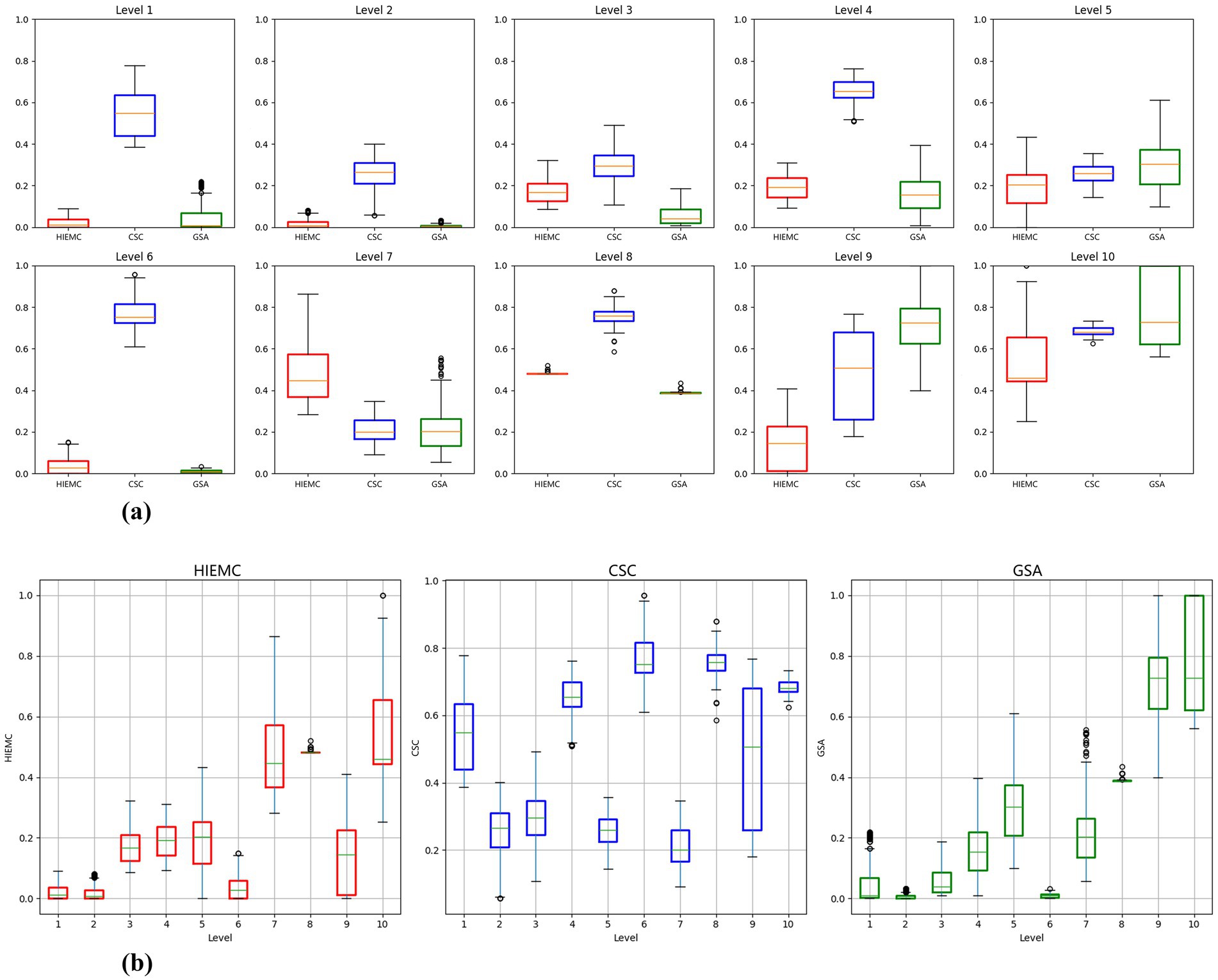
Figure 12. (a) Box plot of sample distribution by level. (b) Box plot of sample distribution by feature.

The second box plot (Figure 12b) further breaks down the distribution of HIEMC, CSC, and GSA within each level. It is evident that lower levels (e.g., Level 1) exhibit lower values for these three features, while higher levels (e.g., Level 10) show greater variability and higher values. This difference in feature distribution highlights the need to consider both environmental factors and social demand factors when evaluating Urban Green Space demand, as higher demand levels are typically associated with more extreme environmental conditions, which require more green space resources for mitigation.

Considering both figures together, the k-means++ algorithm clusters the latent features extracted by the autoencoder, further dividing these different latent features into regions of different demand levels, demonstrating the close connection between HIEMC, CSC, GSA, and Urban Green Space demand. Through the feature learning process, the autoencoder captures the complex nonlinear relationships between these features, providing a more accurate representation of Urban Green Space demand. The clustering results show that in high-demand areas (such as Level 8 to Level 10), the values of HIEMC and GSA significantly increase, and their distribution shows greater fluctuations. Particularly in these regions, the distribution of HIEMC and GSA exhibits higher concentration, reflecting the more severe urban heat island effects and lower green space accessibility levels in these areas.

The distribution of CSC shows some fluctuation, especially between medium and high-demand areas. This fluctuation suggests that CSC concentrations vary significantly across different regions, possibly influenced by various socio-economic and environmental factors. This feature further demonstrates the complexity of Urban Green Space demand, especially in these regions, where the demand for green space is not only related to temperature but also to air quality, environmental pollution, and other factors.

Additionally, we visualized the clustering results in a two-dimensional plane using t-SNE (Figure 13). From the t-SNE visualization, it is evident that the sample groups of different clusters are clearly separated in the two-dimensional space, indicating a high correlation between the latent features and the final clustering results. This clear clustering structure reflects the ability of the extracted features to effectively capture the inherent patterns in the data, providing significant differentiation in high-dimensional space. Therefore, the effectiveness of feature extraction is well validated, demonstrating that these features play an important role in the final clustering task.

Figure 13

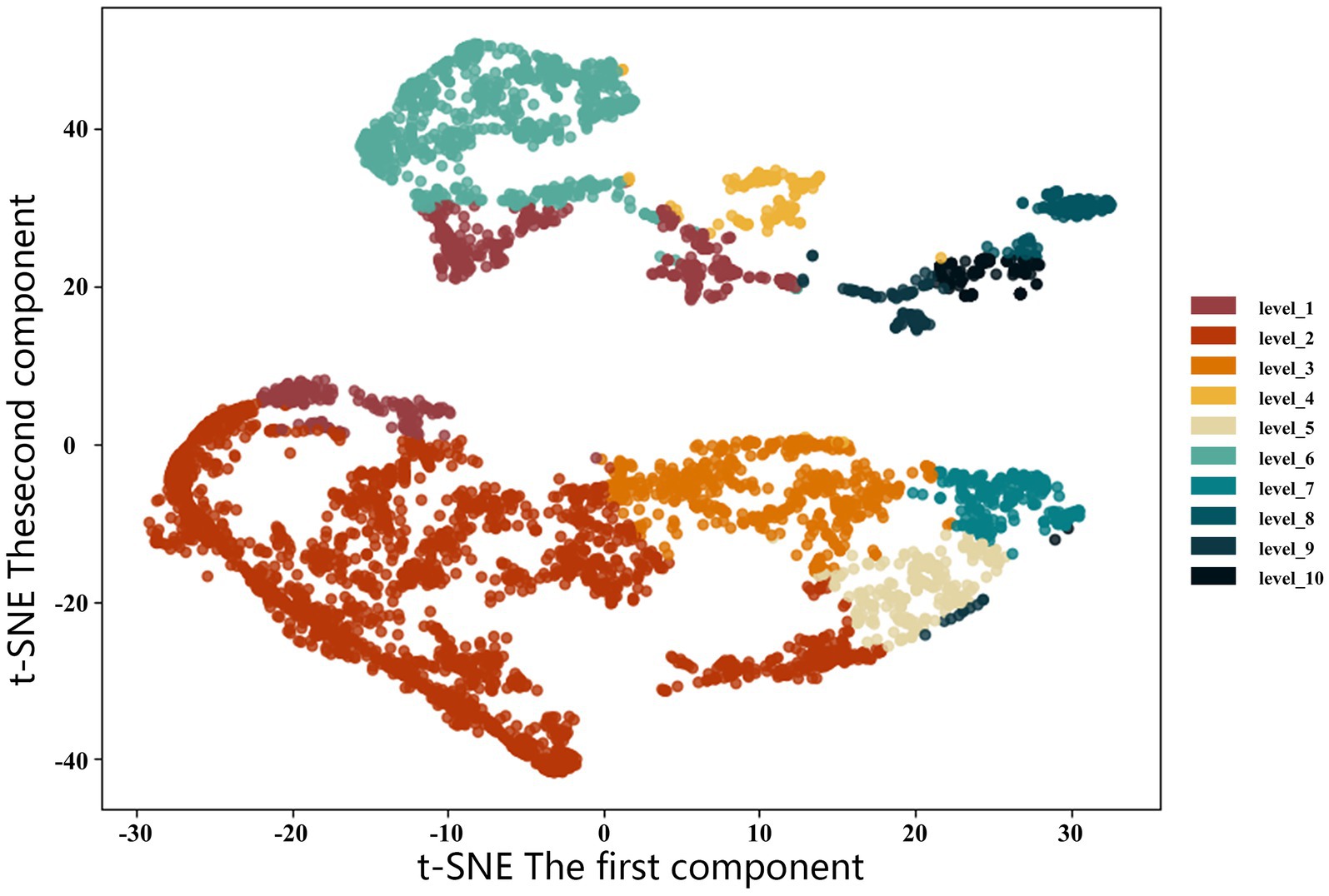
Figure 13. Visualization of clustering results based on t-SNE.

In summary, the relationship between the clustering results and the original data is fully reflected. High-demand regions (Level 8 to Level 10) show significant environmental pressure in the distribution of HIEMC and GSA, indicating a particularly urgent need for green space resources in these areas. The variability of CSC reflects the imbalance between green space resource supply and environmental quality across different regions. Therefore, the optimization and allocation of green space resources in these areas should prioritize environmental characteristics and social needs, particularly in terms of mitigating the urban heat island effect and improving air quality. Through these analyses, we can more clearly understand the relationship between the clustering results and the original data, providing scientific evidence for the rational allocation of Urban Green Space resources.

5.2.2 Interpretative analysis of the autoencoder’s latent space feature extraction

To reveal the relationship between the latent features and the original variables, this study performed an interpretative analysis of the latent features extracted by the autoencoder and the original data (HIEMC, GSA, CSC) using Partial Dependence Plots (PDP). The plots illustrate the dependency relationships between multiple latent features (feature_1 to feature_8) and the original features (HIEMC, GSA, CSC) (Figure 14). PDPs clearly reveal how the latent features extracted by the autoencoder change with variations in the different original data dimensions, by deconstructing functional dependencies of latent features on raw variables, PDP provides direct interpretability for the autoencoder’s black box, explicitly addressing how latent features reflect driving mechanisms of green space demand. Further revealing the contribution of these features to Urban Green Space demand and their inherent correlations.

Figure 14

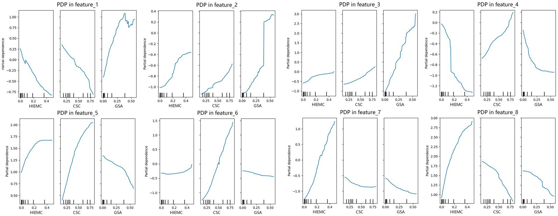
Figure 14. PDP analysis: The impact of original features on latent features.

From the PDP plots, it is evident that the dependencies of different latent features on HIEMC, GSA, and CSC vary significantly. First, for HIEMC (heat island effect mitigating capacity), feature_2 show a positive correlation with HIEMC, particularly at lower HIEMC values, where the latent feature values exhibit relatively stable changes. However, at higher HIEMC values, the latent features show sharp increases or decreases. Feature_7 and feature_8 are the primary driver for HIEMC(heat island effect mitigating capacity), exhibiting steep increases in high HIEMC regions, aligning with observed high-demand zones in urban peripheries. This suggests that as the heat island effect mitigating capacity increases, the latent features of green space demand undergo significant changes, especially in areas with higher urban heat island mitigation capacity, where the variations in green space demand are more sensitive.

For CSC (carbon sequestration capacity), the PDP curves for several latent features (feature_4, feature_5, and feature_6) exhibit strong positive correlations, with the latent feature values increasing as CSC rises. Feature_6 dominates carbon sequestration demand (CSC) with strong positive correlation, explaining carbon hotspot distribution in urban cores. This further indicates a close relationship between increased CSC and green space demand, suggesting that the carbon sequestration capacity of green spaces could play a key role in mitigating carbon emissions in these areas. Lower CSC typically corresponds to higher air pollution and poorer environmental quality, leading to increased demand for green spaces.

For GSA (green space accessibility), in some latent features (such as feature_6, feature_7, feature_8), the latent feature values show a steady decline with increasing green space accessibility, suggesting that the relationship between green space accessibility and demand might be influenced by other factors. However, in some other features (such as feature_1, feature_2, feature_3), as green space accessibility increases, the latent feature values show a sharp increase, reflecting that in areas with high green space accessibility, the demand for green space changes significantly. This is especially true in high-demand urban areas, where the insufficiency of green space supply is more prominent.

Each latent feature (feature_i) captures different patterns of combination between HIEMC, GSA, and CSC to some extent. Some latent features primarily depend on changes in CSC, such as feature_6; others are most sensitive to changes in GSA, such as feature_1; some latent features are most sensitive to HIEMC, such as feature_7; and some latent features show strong sensitivity to two or three variables, although the direction may differ. This multidimensional sensitivity suggests that different latent features may correspond to various urban environmental patterns. For example, “urban heat islands and population concentration areas” may primarily be driven by heat island effects and population density, while “industrial emissions and low-population areas” might be closely linked to carbon dioxide concentration and low population density. “Extremely high-temperature uninhabited zones” might form in areas with extremely high land surface temperatures and low population density. The specific meaning of these patterns requires further verification based on the spatial distribution of these latent features and real urban environmental scenarios.

PDP analysis demonstrates that the autoencoder successfully captures complex nonlinear relationships among original features (HIEMC, GSA, CSC) and their critical roles in Urban Green Space (UGS) demand through latent feature extraction. These latent features not only reflect local data variations but also characterize combined effects of environmental variables (e.g., land surface temperature, carbon concentration, population density) on UGS demand, providing a scientific basis for green space optimization and allocation. Interpretability analysis via PDP confirms the autoencoder’s effectiveness in extracting representative latent features from complex raw data, which accurately reflect multidimensional factors influencing UGS demand and reveal region-specific driving factors behind demand dynamics. Incorporating these latent features into UGS resource allocation will enable more precise demand assessment and resource optimization.

5.3 Choice of activation function

To explore which activation function produces the best training results in the autoencoder, this study investigated the performance of five activation functions in the autoencoder model.

Based on the reconstruction error curves (Figures 15a–e), it is clear that different activation functions exhibit distinct performances during the autoencoder training process. First, the ELU activation function shows large fluctuations in reconstruction error at the early stages of training, but as training progresses, the error rapidly decreases and stabilizes. This indicates that ELU effectively leverages its self-normalizing properties, playing a positive role in network stability, especially in deep networks, and helping the model effectively learn the latent features. Despite the initial fluctuations, ELU achieves a relatively low final reconstruction error, indicating good convergence. Similar to ELU, the LeakyReLU curve also exhibits early fluctuations, followed by a rapid decline and stabilization, showing that LeakyReLU effectively mitigates the “dying neuron” problem, ensuring stable gradient flow. However, the final reconstruction error of LeakyReLU is slightly higher than that of ELU, suggesting that ELU might be more effective than LeakyReLU in optimizing the autoencoder’s performance in certain feature learning tasks. Regarding ReLU, its performance is similar to LeakyReLU, with a relatively quick initial convergence, but it ultimately results in slightly higher error levels and slower convergence, likely due to the gradient vanishing problem that ReLU can suffer from in deep networks. In contrast, the SELU activation function demonstrated the best performance among all the functions, with very smooth error reduction throughout the training process and the lowest final reconstruction error. This can be attributed to the self-normalizing properties of SELU, which maintains the mean and variance of the network, ensuring more efficient feature learning, especially in deeper network structures. Lastly, the Tanh activation function performed relatively poorly; although it avoids the “dying neuron” issue seen with ReLU, its gradient saturation characteristics lead to slow training and higher final reconstruction errors.

Figure 15

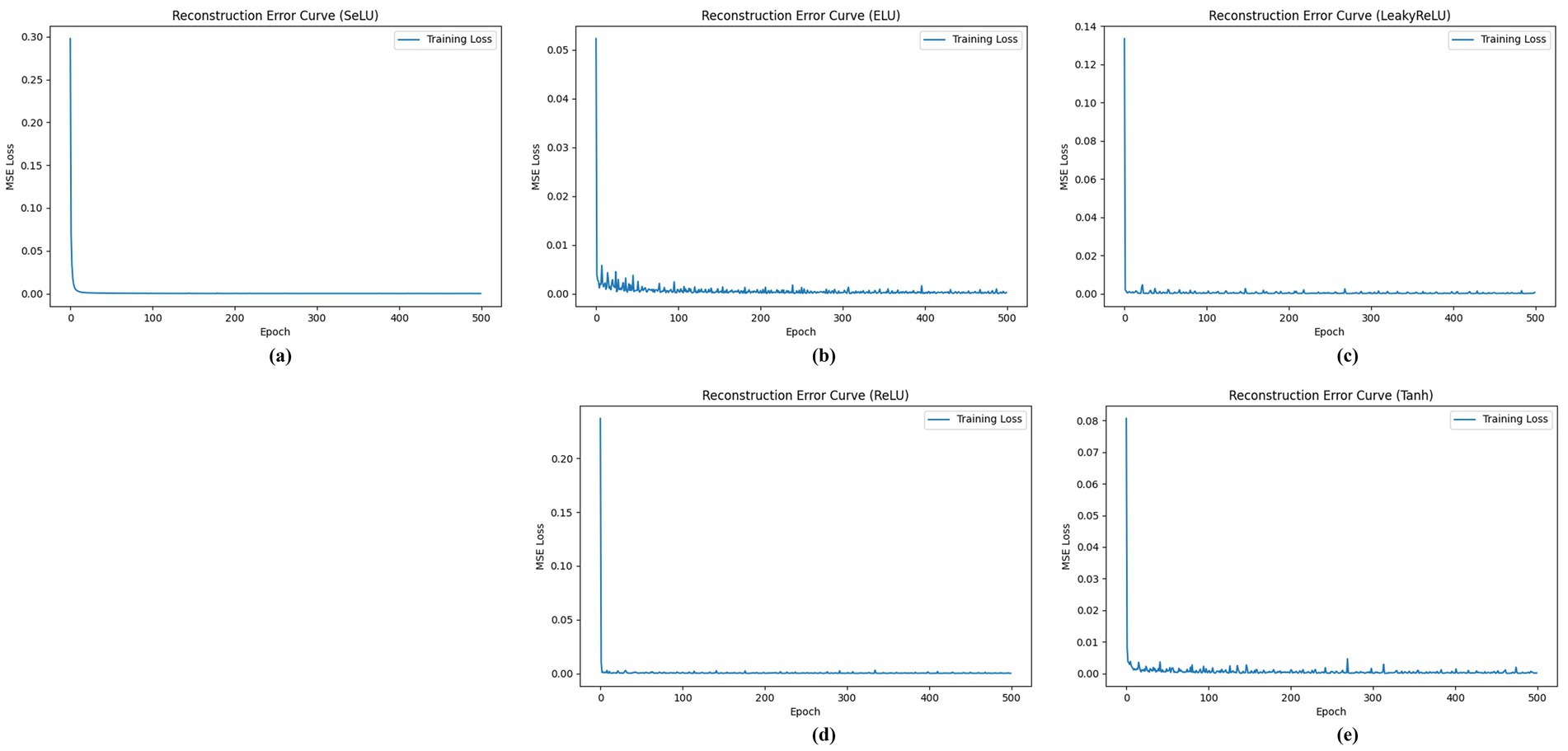
Figure 15. Training loss trend of the autoencoder using different activation functions. (a) SeLU. (b) ELU. (c) LeakyReLU. (d) ReLU. (e) Tanh.

In conclusion, SELU provided the best performance in this study and is suitable for use in deep autoencoders. LeakyReLU and ReLU are more robust alternatives, suitable when SELU conditions are not met. Tanh, however, performed worse than the other activation functions, especially in deep networks, where its gradient issues may result in poor convergence.

5.4 Limitations and future research directions

This study advances urban green space demand assessment through an autoencoder-based framework, yet several limitations require acknowledgement:

This study excludes the critical environmental and socioeconomic determinants, specifically real-time air quality indices (PM_2.5 and NO₂ concentrations), vegetation health metrics (NDVI and EVI), and economic vitality indicators (nighttime light intensity and POI density), and restricts the model’s capacity to characterize demand heterogeneity in commercial-industrial zones. This omission compromises the generalizability of demand predictions in rapidly developing urban peripheries where anthropogenic emissions and land-use intensification exhibit nonlinear interactions.

Although the 8-dimensional latent features extracted by the autoencoder demonstrate strong discriminatory power, the nonlinear mapping between input variables (HIEMC/GSA/CSC) and encoded representations remains opaque. This obscures mechanistic interpretation of demand drivers, hindering the translation of clustering results into prioritized planning interventions.

Despite implementing IQR-based outlier detection and Robust scaler normalization, high-frequency noise in remotely sensed LST data (attributable to atmospheric transient effects) propagates through the unsupervised pipeline. This phenomenon introduces instability in cluster boundary delineation, particularly in regions with microclimate variability.

Future research trajectories will address these constraints through:

5.4.1 Multidimensional indicator integration

A fused sensing framework will assimilate Sentinel-5P tropospheric NO₂ column density, VIIRS nighttime light composites (500 m), and Gaofen-2 NDVI time-series (8 m) to quantify pollution exposure, economic activity, and vegetation stress. This expansion will enable demand calibration in emission-intensive manufacturing districts currently underrepresented in the model.

5.4.2 Spatiotemporal graph neural networks

ST-GNN architectures with attention-based LSTM modules will be deployed to capture demand trajectories across over 5-year observation windows. Pilot implementation will target Chengdu’s Tianfu New Area, evaluating green space allocation efficiency against urban expansion rates derived from Landsat-derived impervious surface maps.

5.4.3 Hybrid explainability framework

SHAP (Shapley Additive explanations) will quantify feature contributions to latent dimensions, generating spatially explicit attribution maps. Integration with existing PDP analysis will establish causal pathways between industrial emissions and high-demand clusters.

5.4.4 Adaptive noise suppression

Discrete wavelet packet transforms (db8 mother wavelet) will decouple seasonal noise (summer LST anomalies) from persistent demand signals prior to autoencoder training. Thresholding criteria will optimize signal-to-noise ratios in MODIS LST collections using Stein’s Unbiased Risk Estimate.

These advancements will establish a dynamic urban green infrastructure assessment system.

6 Conclusion

This study proposes an autoencoder-based framework for evaluating Urban Green Space demand and applies it to the green space demand analysis of the central urban area of Chengdu. By integrating multidimensional ecological and social indicators such as population density, land surface temperature (LST), and carbon dioxide concentration, we have innovatively overcome the limitations of traditional assessment methods, where ecological and social dimensions are considered separately. This framework enables a deeper evaluation of urban green space demand. The approach not only provides more accurate and comprehensive analysis of green space demand variations but also significantly enhances the scientific basis for urban green space resource allocation.

Through the training and feature extraction of the autoencoder model, we successfully mined multidimensional latent features from the data and used these features to conduct a detailed assessment of green space demand in the central urban area of Chengdu. The results indicate that carbon sequestration capacity, heat island effect mitigation, and green space accessibility are key factors influencing green space demand. In particular, urban core areas with high population density and carbon dioxide emissions show an especially urgent demand for green space. Green space demand in these areas is crucial not only for ecological improvements but also for enhancing the quality of daily life and the physical and mental health of residents.

The results further show that green space demand based on carbon sequestration capacity is primarily concentrated around the city center and transportation hubs. These areas, due to high carbon dioxide emissions, urgently require more green spaces to alleviate environmental pressure. In contrast, demand based on heat island effect mitigation is mainly concentrated in the expanding urban fringe, where higher temperatures necessitate more green spaces to regulate the microclimate. Demand based on green space accessibility is concentrated in densely populated areas, especially in neighborhoods where the green space supply is insufficient. These analyses provide urban planners with a comprehensive green space demand map that can effectively guide the optimization of green space resource allocation.

The study’s findings also demonstrate that the integration and analysis of multidimensional data using autoencoder technology can reveal the complexity and spatial heterogeneity of Urban Green Space demand. Specifically, the autoencoder captures nonlinear relationships within the data, accurately reflecting the deep connections between urban green space demand and environmental variables such as temperature, carbon dioxide concentration, and population density. Compared to traditional methods, the autoencoder-based framework not only improves model accuracy and uncovers deep interactions among environmental variables but also enhances the spatial precision of green space demand evaluation, providing a scientific foundation for the rational allocation of urban green space resources.

Overall, this study not only offers a new approach and methodology for evaluating urban green space demand but also provides an important reference for future research in areas such as urban ecological planning, green infrastructure development, and climate adaptation planning. The research results indicate that through deep analysis of the interaction between ecological and social dimensions, it is possible to better identify and address spatial disparities in urban green space demand, thereby providing solid theoretical support for achieving sustainable urban development goals.

Data availability statement

The data analyzed in this study is subject to the following licenses/restrictions: Data will be made available on request. Requests to access these datasets should be directed to Dongzhi Luo, bHVvZHpoMjAyNEBsenUuZWR1LmNu.

Author contributions

WQ: Writing – review & editing, Supervision, Project administration, Data curation, Writing – original draft, Funding acquisition. DL: Writing – original draft, Methodology, Investigation, Conceptualization, Validation, Software, Writing – review & editing.

Funding

The author(s) declare that financial support was received for the research and/or publication of this article. This work was supported by [Liaoning Provincial Science and Technology Department] under Grant [No. 2023-MSBA-057].

Conflict of interest

The authors declare that the research was conducted in the absence of any commercial or financial relationships that could be construed as a potential conflict of interest.

Generative AI statement

The authors declare that no Gen AI was used in the creation of this manuscript.

Any alternative text (alt text) provided alongside figures in this article has been generated by Frontiers with the support of artificial intelligence and reasonable efforts have been made to ensure accuracy, including review by the authors wherever possible. If you identify any issues, please contact us.

Publisher’s note

All claims expressed in this article are solely those of the authors and do not necessarily represent those of their affiliated organizations, or those of the publisher, the editors and the reviewers. Any product that may be evaluated in this article, or claim that may be made by its manufacturer, is not guaranteed or endorsed by the publisher.

References

Bhandari, S., and Zhang, C. (2022). Urban green space prioritization to mitigate air pollution and the urban heat island effect in Kathmandu Metropolitan City, Nepal. Land 11:2074. doi: 10.3390/land11112074

Crossref Full Text | Google Scholar

Bhattacharjee, A., Popov, A. A., Sarshar, A., and Sandu, A. (2024). Improving the adaptive moment estimation (ADAM) stochastic optimizer through an implicit-explicit (IMEX) time-stepping approach. arXiv. doi: 10.48550/ARXIV.2403.13704

Crossref Full Text | Google Scholar

Chen, J., Wang, C., Zhang, Y., and Li, D. (2022). Measuring spatial accessibility and supply-demand deviation of urban green space: a mobile phone signaling data perspective. Front. Public Health 10:1029551. doi: 10.3389/fpubh.2022.1029551

PubMed Abstract | Crossref Full Text | Google Scholar

Cheshmehzangi, A., Butters, C., Xie, L., and Dawodu, A. (2021). Green infrastructures for urban sustainability: issues, implications, and solutions for underdeveloped areas. Urban For. Urban Green. 59:127028. doi: 10.1016/j.ufug.2021.127028

Crossref Full Text | Google Scholar

Cohn, R., and Holm, E. (2021). Unsupervised machine learning via transfer learning and k-means clustering to classify materials image data. Integr. Mater. Manuf. Innov. 10, 231–244. doi: 10.1007/s40192-021-00205-8

Crossref Full Text | Google Scholar

Czesak, B., and Różycka-Czas, R. (2025). Assessing accessibility and crowding in urban green spaces: a comparative study of approaches. Landsc. Urban Plan. 257:105301. doi: 10.1016/j.landurbplan.2025.105301

Crossref Full Text | Google Scholar

Dong, Q., Lu, H., Luo, X., He, P., Li, D., Wu, L., et al. (2023). Evaluation and optimization of green space fairness in urban built-up areas based on an improved supply and demand model: a case study of Chengdu, China. Sustainability 15:15014. doi: 10.3390/su152015014

Crossref Full Text | Google Scholar

Du, C., Ge, S., Song, P., Jombach, S., Fekete, A., and Valánszki, I. (2025). Optimizing urban green spaces for vegetation-based carbon sequestration: the role of landscape spatial structure in Zhengzhou parks, China. Forests 16:679. doi: 10.3390/f16040679

Crossref Full Text | Google Scholar

Gao, S., Tao, P., Zhao, Z., Dong, X., Li, J., and Yao, P. (2024). Estimation and differential analysis of the carbon sink service radius of urban green spaces in the Beijing plain area. Sustainability 16:1406. doi: 10.3390/su16041406

Crossref Full Text | Google Scholar

Hazra, A., Choudhary, P., Inunganbi, S., and Adhikari, M. (2020). Bangla-Meitei Mayek scripts handwritten character recognition using convolutional neural network. Appl. Intell. 51, 2291–2311. doi: 10.1007/s10489-020-01901-2

Crossref Full Text | Google Scholar

Huang, S., Wang, C., Deng, M., and Chen, Y. (2023). Coupling coordination between park green space (PGS) and socioeconomic deprivation (SED) in high-density city based on multi-scale: from environmental justice perspective. Land 12:82. doi: 10.3390/land12010082

Crossref Full Text | Google Scholar

Jin, Y., He, R., Hong, J., Luo, D., and Xiong, G. (2023). Assessing the accessibility and equity of urban green spaces from supply and demand perspectives: a case study of a mountainous city in China. Land 12:1793. doi: 10.3390/land12091793

Crossref Full Text | Google Scholar

Kim, S. W., and Brown, R. D. (2021). Urban heat island (UHI) variations within a city boundary: a systematic literature review. Renew. Sust. Energ. Rev. 148:111256. doi: 10.1016/j.rser.2021.111256

Crossref Full Text | Google Scholar

Liu, J., Li, C., and Yang, W. (2018). Supervised learning via unsupervised sparse autoencoder. IEEE Access 6, 73802–73814. doi: 10.1109/ACCESS.2018.2884697

Crossref Full Text | Google Scholar

Long, Y., Wu, Y., Huang, L., Aleksejeva, J., Iossifova, D., Dong, N., et al. (2024). Assessing urban livability in Shanghai through an open-source data-driven approach. NPJ Urban Sustain. 4:7. doi: 10.1038/s42949-024-00146-z

Crossref Full Text | Google Scholar

Lopes, H. S., Silva, P. F., Pinto, B. G., Cuevas, P. D., Ribeiro, V., and Remoaldo, P. (2025). Urban heat stress in the context of socioeconomic and environmental challenges: heat risk analysis and online surveys in northwestern Portugal. Int. J. Disaster Risk Reduct. 120:105384. doi: 10.1016/j.ijdrr.2025.105384

Crossref Full Text | Google Scholar

Lopes, H. S., Vidal, D. G., Cherif, N., Silva, L., and Remoaldo, P. C. (2025). Green infrastructure and its influence on urban heat island, heat risk, and air pollution: a case study of Porto (Portugal). J. Environ. Manag. 376:124446. doi: 10.1016/j.jenvman.2025.124446

PubMed Abstract | Crossref Full Text | Google Scholar

Lu, Y., Gould, S., and Ajanthan, T. (2023). Bidirectionally self-normalizing neural networks. Neural Netw. 167, 283–291. doi: 10.1016/j.neunet.2023.08.017

PubMed Abstract | Crossref Full Text | Google Scholar

Ouyang, L., Yang, Y., Zhiqiang, W., Jiang, Q., and Qiao, R. (2024). Towards inclusive urbanism: an examination of urban environment strategies for enhancing social equity in Chengdu's housing zones. Sustain. Cities Soc. 107:105414. doi: 10.1016/j.scs.2024.105414

Crossref Full Text | Google Scholar

Permata, A. P. M., Buchori, I., and Kurniati, R. (2021). Adequacy measurement of public green open space (GOS) in absorbing carbon dioxide (CO₂) emissions from transportation activities in Tampan district, Pekanbaru. IOP Conf Ser Earth Environ Sci 896:012015. doi: 10.1088/1755-1315/896/1/012015

Crossref Full Text | Google Scholar

Pratama, K., and Kang, D.-K. (2020). Trainable activation function with differentiable negative side and adaptable rectified point. Appl. Intell. 51, 1784–1801. doi: 10.1007/s10489-020-01885-z

Crossref Full Text | Google Scholar

Qiao, Z., Jia, R., Liu, J., Gao, H., and Wei, Q. (2024). Remote sensing-based analysis of urban heat island driving factors: a local climate zone perspective. IEEE J. Sel. Top. Appl. Earth Observ. Remote Sens. 17, 17337–17348. doi: 10.1109/JSTARS.2024.3462537

Crossref Full Text | Google Scholar

Rochmawati, N., Hidayati, H. B., Yamasari, Y., Tjahyaningtijas, H. P. A., Yustanti, W., and Prihanto, A. (2021). Analisa Learning Rate dan Batch Size pada Klasifikasi Covid menggunakan deep learning Dengan optimizer Adam. J. Inf Eng Educ Technol 5, 44–48. doi: 10.26740/jieet.v5n2.p44-48

Crossref Full Text | Google Scholar

Sakketou, F., and Ampazis, N. (2019). “On the invariance of the SELU activation function on algorithm and Hyperparameter selection in neural network recommenders” in IFIP advances in information and communication technology (Cham: Springer International Publishing), 673–685.

Google Scholar

Tan, C., Liu, C., Yang, H., Wang, N., and Liu, Y. (2022). From service capacity to spatial equity: exploring a multi-stage decision-making approach for optimizing elderly-care facility distribution in the city Centre of Tianjin, China. Sustain. Cities Soc. 85:104076. doi: 10.1016/j.scs.2022.104076

Crossref Full Text | Google Scholar

Vaishnavi, V. S., Reddy, S., Deepa, K., and Sailaja, V. (2024). “Assessing CO2 gas emission in residential areas: implications for sustainable urban development” in 2024 5th international conference on smart electronics and communication (ICOSEC), vol. 2024 (Trichy, India: IEEE Xplore), 302–307.

Google Scholar

Wang, C., Guo, M., Jin, J., Yang, Y., Ren, Y., Wang, Y., et al. (2022). Does the spatial pattern of plants and green space affect air pollutant concentrations? Evidence from 37 garden cities in China. Plants 11:212847. doi: 10.3390/plants1121284

Crossref Full Text | Google Scholar

Wang, S., Huang, H., Hao, C., Cao, L., and Liu, T. (2019). Sensitivity microscale of urban heat island reduction by green space. Open House Int. 44, 147–151. doi: 10.1108/OHI-03-2019-B0034

Crossref Full Text | Google Scholar

Wen, W., and Zheng, T. (2023). Establishing a "dynamic two-step floating catchment area method" to assess the accessibility of urban green space in Shenyang based on dynamic population data and multiple modes of transportation. Urban For. Urban Green. 82:127893. doi: 10.1016/j.ufug.2023.127893

PubMed Abstract | Crossref Full Text | Google Scholar

Xie, H., Wang, X., Hu, X., Shi, Z., Lin, H., Xie, X., et al. (2023). Exploring urban green space optimization of the urban walking life circle in Fuzhou, China. Int. J. Environ. Res. Public Health 20:1180. doi: 10.3390/ijerph20021180

PubMed Abstract | Crossref Full Text | Google Scholar

Xu, L., Fang, K., Huang, Y., and Xu, S. (2023). Demand priority of green space from the perspective of carbon emissions and storage. Sustainability 15:11199. doi: 10.3390/su151411199

Crossref Full Text | Google Scholar

Xu, N., and Wang, P. (2024). Evolutionary characteristics of urban public space accessibility for vulnerable groups from a perspective of temporal–spatial change: evidence from Nanjing old city, China. Land 13:998. doi: 10.3390/land13070998

Crossref Full Text | Google Scholar

Xue, K., Yu, K., and Zhang, H. (2023). Accessibility analysis and optimization strategy of urban green space in Qingdao City Center, China. Ecol. Indic. 156:111087. doi: 10.1016/j.ecolind.2023.111087

Crossref Full Text | Google Scholar

Zhang, Y., Chen, C., Li, Z., Ding, T., Wu, C., Kingma, D. P., et al. (2024). Adam-mini: use fewer learning rates to gain more (版 7). arXiv. doi: 10.48550/ARXIV.2406.16793

Crossref Full Text | Google Scholar

Zhang, Y., Ge, J., Wang, S., and Dong, C. (2025). Optimizing urban green space configurations for enhanced heat island mitigation: a geographically weighted machine learning approach. Sustain. Cities Soc. 119:106087. doi: 10.1016/j.scs.2024.106087

Crossref Full Text | Google Scholar

Zhang, G., Su, Y., Wang, Z., Chen, Y., Wan, J., and Bai, H. (2024). Spatial–temporal evolution and driving force analysis of blue–green space in the Chengdu–Chongqing economic circle, China. Land 13:1733. doi: 10.3390/land13111733

Crossref Full Text | Google Scholar

Zhao, K., Chen, C., Wang, J., Liu, K., Wu, F., and Cao, X. (2024). Examining the spatial mode, supply–demand relationship, and driving mechanism of urban park green space: a case study from China. Forests 15:131. doi: 10.3390/f15010131

Crossref Full Text | Google Scholar

Zhao, W., Li, X., Zhang, L., Peng, L., Liu, Y., Wang, Z., et al. (2023). The multi-scale spatial heterogeneity of ecosystem services’ supply–demand matching and its influencing factors on urban green space in China. Forests 14:2091. doi: 10.3390/f14102091

Crossref Full Text | Google Scholar