Leveraging productivity indicators for anomaly detection in swine breeding herds with unsupervised learning

Introduction: In swine disease surveillance, obtaining labeled data for supervised learning models can be challenging because many farms lack standardized diagnostic routines and consistent health monitoring systems. Unsupervised learning is particularly suitable in such scenarios because it does not require labeled data, allowing for detecting anomalies without predefined labels. This study evaluates the effectiveness of unsupervised machine learning models in detecting anomalies in productivity indicators in swine breeding herds.

Methods: Anomalies, defined as deviations from expected patterns, were identified in indicators such as abortions per 1000 sows, prenatal losses, preweaning mortality, total born, liveborn, culled sows per 1000 sows, and dead sows per 1000 sows. Three unsupervised models - Isolation Forest, Autoencoder, and K-Nearest Neighbors (KNN) - were applied to data from two swine production systems. The herd-week was used as the unit of analysis, and anomaly scores above the 75th percentile were used to flag anomalous weeks. A permutation test assessed differences between anomalous and non-anomalous weeks. Performance was evaluated using F1-score, precision, and recall, with true anomalous weeks defined as those coinciding with reported health challenges, including porcine reproductive and respiratory syndrome (PRRS) and Seneca Valley virus outbreaks. A total of 8,044 weeks were analyzed.

Results: The models identified 336 anomalous weeks and 1,008 non-anomalous weeks in Production System 1, and 1,675 anomalous weeks and 5,025 non-anomalous weeks in Production System 2. The results from the permutation test revealed significant differences in productivity indicators between anomalous and non-anomalous weeks, especially during PRRS outbreaks, with more subtle changes observed during Seneca Valley virus outbreaks. The models performed well in detecting the PRRSV anomaly, achieving perfect precision (100%) across all models for both production systems. For anomalies like SVV the models showed lower performance compared to PRRSV.

Discussion: These findings suggest that unsupervised machine learning models are promising tools for early disease detection in swine herds, as they can identify anomalies in productivity data that may signal health challenges.

Introduction

The global pork production industry is crucial for food security, with the United States being one of the top producers and exporters (55). Maintaining herd health is essential for economic success in this sector. However, challenges persist, with diseases having a major impact on the swine production systems. Porcine reproductive and respiratory syndrome virus (PRRSV) was estimated to cost the U.S. swine industry around $1.2 billion annually (1). In the Netherlands, PRRSV outbreaks were estimated to cause an average loss of $131.2 per sow per outbreak (2). The introduction of the porcine epidemic diarrhea virus (PEDV) in the U.S. in 2013 caused the loss of seven million pigs (3), and a study made in the U.S. estimated the cost to be $300,000 per year for a single 700-sow farrow-to-finishing herd (4). In Europe the cost of classical swine fever outbreaks in the Netherlands and Belgium was estimated as $2.3 billion and $11.5 million, respectively. In Romania, African swine fever led to a reduction of the national pig population by 8.44%, with 348,691 pigs slaughtered (5), and a study estimated a loss of $15 billion in a scenario where African swine fever was introduced in the U.S. and controlled and estimated a loss of $50 billion in a scenario where the disease spread to feral swine and it was not controlled (6). These are some examples of the economic impact of diseases on production, and with that, it is important to consider strategies to detect early anomalies, trigger outbreak investigation, and implement measures to avoid the further spread of pathogens.

Anomalies are data points that deviate from values expected under a given model or contextual distribution. Such deviations may arise from measurement errors, atypical operating conditions, or previously unknown processes affecting the system (7). In the swine industry, an anomaly refers to an unexpected value in productivity indicators, which can arise for multiple reasons like animal management and husbandry, human error in data collection, environmental changes, and health-related factors. Numerous studies have demonstrated that syndromic surveillance is highly effective in detecting health-related events in swine breeding herds. For example, using statistical process control (SPC) charts to track productivity indicators has enabled the detection of deviations associated with PRRSV outbreaks early, often before routine diagnostic monitoring (8–10). These studies indicated that observing multiple productivity indicator patterns allows early detection of health challenges. Apart from these methods, anomaly detection also relies on methods such as time series (11, 12), supervised machine learning (13), and unsupervised learning (7, 14).

Unsupervised learning involves using algorithms to identify patterns or structures in datasets without any external guidance or labeled information (15). It can be used for different purposes, and while there is limited information on its use for disease surveillance in the swine industry, it has been utilized to test lying patterns in pigs by combining image processing, unsupervised clustering, and central neural networks with support vector machine classification (16). Unsupervised learning was also used to identify variables of economically important performance traits in swine (17) and to identify evolving phenotypes after trauma using principal component analysis (18). Moreover, unsupervised learning was used to describe the network structure and spatiotemporal characteristics of swine shipment using factor analysis for mixed data and hierarchical clustering (19). In the context of swine disease surveillance, obtaining labeled data for supervised learning models can be difficult because, in many cases, farms do not have established diagnostic routines or consistent health monitoring systems to generate reliable labels for anomalies, making it hard to train supervised models to detect these anomalies reliably. For this reason, unsupervised models are an attractive option since they do not require labeled data, allowing them to identify unknown anomalies that supervised learning might miss if not predefined in the labels (20–22). In this study, it was hypothesized that unsupervised models could be used to detect anomalies in production indicators (abortions per 1,000 sows, prenatal losses, preweaning mortality, total born, liveborn, culled sows per 1,000 sows and dead sows per 1,000 sows) commonly affected when there is disease introduction in swine breeding herds (23, 24) from farms that lack active surveillance or sufficient labeled data. These models could identify deviations from normal production patterns that might go unnoticed and could trigger further investigation of potential health challenges. This provides insight into how unsupervised learning might perform when applied to real-world settings, where labels are often unavailable, and emphasizes the importance of these models in filling the gap when traditional supervised learning approaches cannot be applied.

The primary goal of this study was to evaluate the efficacy of unsupervised machine learning models in detecting anomalies in the productivity indicators of swine breeding herds. Efficacy in this context was defined by the model's ability to identify anomalies indicative of health challenges based on deviations in productivity indicators. Specifically, the study aimed to (1) compare unsupervised models in terms of anomaly detection across anomalous and non-anomalous weeks and (2) examine the potential of unsupervised models to uncover hidden anomalies that could signal emerging health challenges, even in the absence of known disease labels.

Methods

Overview of the study

Data from two distinct production systems were used in the study, and the models were implemented for each system individually, allowing for a comprehensive evaluation across different settings, using the herd-week as the unit of analysis. Unsupervised learning offers benefits since it does not depend on labeled data, enabling the discovery of previously unidentified anomalies that supervised methods might overlook. In this study, three unsupervised models were implemented—Isolation Forest, Autoencoder, and K-nearest neighbors (KNN) to identify anomalous weeks (weeks that had anomaly scores above the 75th percentile) in productivity indicators without providing the models with prior knowledge of health challenges. Following model implementation, the identified anomalous weeks were compared with known health challenges to evaluate the potential of these models for syndromic surveillance in swine herds.

Data source

The data used in this study originated from an ongoing surveillance system that monitors weekly productivity data from swine breeding herds from two swine production systems across the United States (FieldEPi Swine Data Surveillance System, https://fieldepi.org/ongoing-monitoring-of-production-data-breeding-sows/). This system collects weekly productivity data via automated emails or Application Programming Interface (API), securely stored on a dedicated server. This robust surveillance infrastructure and ongoing communication with participants enables the aggregation of sow performance monitoring data that contains productivity data on different indicators related to breeding, farrowing, and weaning performance, from various production systems, facilitating both retrospective and prospective studies.

Inclusion criteria and dataset

The breeding herds selected for this analysis followed the inclusion criteria: (a) willingness to share weekly productivity indicators, (b) being operated at a continuous breeding-farrowing fashion (i.e., not batch farrowing), (c) willingness to share diagnostic data, vaccination data, and reports from health challenges from field veterinarians, (d) having at least 21 weeks of data, comprising a full production cycle in breeding herds.

The dataset was built with data from two production systems. Production System 1 had an inventory of 24,847 sows distributed in seven farms and 1,344 herd-weeks (i.e., weekly indicators reported per herd on a calendar-week basis) of productivity data. Production System 2 had an inventory of 205,257 sows, 42 farms, and 6,700 herd-weeks of productivity data. The indicators used as input for the analysis were the weekly abortions per 1,000 sows, weekly average number of total pigs born per litter, weekly average number of liveborn piglets per litter, weekly percentage of prenatal losses defined as the difference between total born and born alive per litter, weekly preweaning mortality percentage from pigs born alive, weekly females culled per 1,000 sows, and weekly dead sows per 1,000 sows.

Data on diagnostics provided by the production systems and reports of health challenges made by the veterinarians were also collected. The reported outbreaks comprised the following pathogens: Seneca Valley virus (SVV) and PRRSV. The impact of a disease on animals does not occur solely during the week of the outbreak. To reflect this more accurately, each disease's incubation and resolution periods were considered and added to the dataset as indicated in the literature. A period of 8 weeks before and 15 weeks after the week of a PRRSV outbreak positive diagnostic was considered as weeks within the outbreak period (10, 25). For SVV, the outbreak period was considered as the week before the positive diagnostic and 2 weeks after (25–27).

Unsupervised learning for anomaly detection

The implementation and analysis using the three unsupervised models were done in the statistical programming environment R Statistical Software (v4.4.0; (56)) and Microsoft Excel.

Isolation Forest

Isolation Forest operates by recursively partitioning the data using randomly selected features, isolating anomalous values faster than traditional methods such as clustering or distance-based techniques. An isolation tree is constructed by recursively partitioning the dataset based on randomly selected attributes and threshold values until reaching a specified height limit or a single data point (28, 29). This process generates a binary tree structure. To quantify anomalies, a ranking method evaluates each data point's path length from the root to the leaf node. The anomaly score [0, 1] is calculated using the formula:

$\begin{array}{l}s(x,n)=2-E(h(x))\times c(n),\end{array}$

where E(h(x)) is the expected path length, n is the testing data size, and c(n) represents the average path length for unsuccessful searches in a binary search tree. Points with scores close to 1 are classified as anomalies, while those below 0.5 are considered normal (28).

A 10-fold cross-validation procedure was set up using the caret package (30), allowing for robust hyperparameter tuning. A set of hyperparameters for the Isolation Forest model were defined using a grid, with sample size (256, 500, and 1,000) and number of trees (100, 200, and 300). Package purrr (31) was used to iterate through each combination of hyperparameters, training and evaluating the model on the training data and calculating the mean anomaly score for each fold. During cross-validation, the average anomaly score across folds was used as a relative performance metric for model selection. While this metric does not directly measure detection accuracy, it provides a consistent basis to compare configurations in the absence of a large labeled dataset. The small number of labeled anomalies was later used to evaluate the models' ability to flag known health-related anomalies, while also assessing their potential to uncover hidden or emerging anomalies. After cross-validation, the optimal hyperparameters, determined by the lowest average anomaly score, were selected, with a sample size equal to 700 and a number of trees equal to 100 (Table 1). The final model was trained with the best hyperparameters, and anomaly scores were predicted. Finally, anomaly scores were compared to a threshold using the 75th percentile of the anomaly scores to classify points as anomalies. The thresholding step was applied post hoc to the final trained model, rather than during cross-validation. Cross-validation was used exclusively for hyperparameter tuning, while the 75th percentile cutoff was applied once to the anomaly scores from the fully trained model. This separation ensured that thresholding did not influence model selection, but rather served as the final classification step. This approach used the isotree package (32) for anomaly detection. Using a threshold for anomaly detection has been an approach used in the literature (33). By using the 75th percentile as a threshold for the anomaly scores, it is possible to detect the most extreme outliers without being overly restrictive or lenient. This choice provided a simple and interpretable threshold that could be applied consistently across models. Percentile-based thresholding is commonly used in unsupervised settings where labeled anomalies are limited, as it allows for empirical selection of a cutoff based on the observed distribution of anomaly scores (34–36).

Table 1

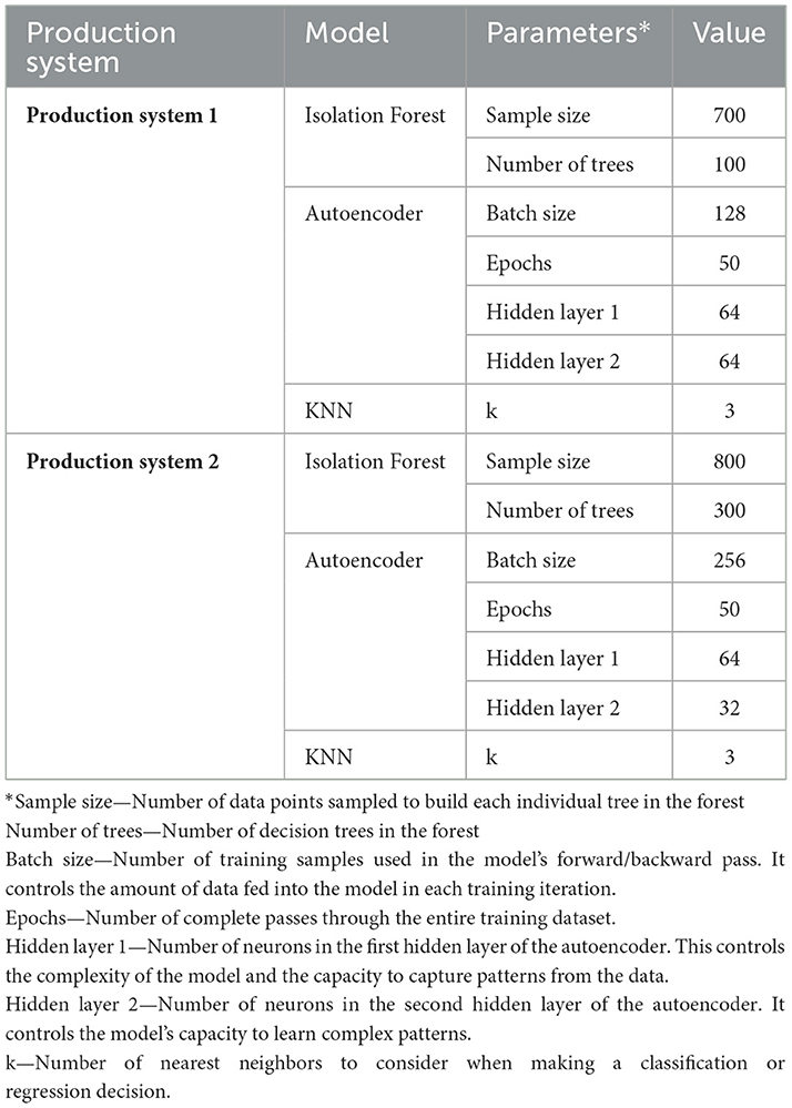
Table 1. Parameter values for the different models, or each production system.

K-nearest neighbor

K-nearest neighbor (KNN), a clustering technique, can be also implemented for anomaly detection with unsupervised learning. The principle behind this model is to find k predefined number of training samples that are closest in the distance to a new point and predict a label for the new point using the samples (37). The anomaly score [0, ∞] is calculated as follows:

$\begin{array}{l}kNN(xq,X,k)=\frac{1}{k}{\sum }_{x\in Nk(X,xq)}\left|\right|xq-x\left|\right|2,\end{array}$

where Nk(X, xq) is the set of k nearest neighbors of xq, xq is the query data, and X is the search space (38).

In this study, a KNN algorithm was employed for anomaly detection using the kknn (39), and FNN (40) packages in R. First, a parameter grid was defined for tuning the number of neighbors (k), ranging from 3 to 10. A 10-fold cross-validation was used to evaluate different configurations, with each fold generating an anomaly score based on the sum of distances to the k-nearest neighbors. The KNN model was trained, utilizing a Euclidean distance (specified via the distance = 2 argument) and a rectangular kernel to compute the distances. The anomaly scores for each fold were computed as the row sums of these distances, representing the degree of “anomalousness” of each data point. The results of each fold were stored and averaged across all folds to identify the optimal hyperparameter (k) based on the lowest average anomaly score. After selecting the best k (k = 3), the final model was trained on the entire training dataset (Table 1). The FNN package was then used to calculate the final distances, with anomaly scores derived from the summed distances to the nearest neighbors. To classify anomalies, the 75th percentile of the anomaly scores was used as a threshold, and data points above this threshold were labeled as anomalies (33–36).

Autoencoders

Autoencoders, a type of neural network, learn to compress and reconstruct input data by minimizing the reconstruction error or anomaly score; anomalies are detected based on poor reconstruction performance (the difference between the input and the output), as anomalies do not fit the learned patterns (22). The reconstruction error or anomaly score [0, ∞] is calculated as follows:

$\begin{array}{l}\text{S}(\text{x}\text{i})=||\text{x}i-\text{g}\text{u}(\text{f}\text{w}(\text{x}\text{i}))||,\end{array}$

where xi is the input data, gu is the decoder function, fw is the encoder function. Anomaly detection using autoencoders operates on the premise that anomalies are linked to higher values of S(xi), reconstruction losses, while normal data is associated with lower reconstruction losses (22).

A 10-fold cross-validation procedure was set up allowing for hyperparameter tuning. A grid of hyperparameters was defined, including various configurations for the number of hidden units in the two layers, hidden layer 1 (64, 128, 256), and hidden layer 2 (32, 64), the number of epochs (50, 100), batch size (128, 256), and learning rate (0.001, 0.0001). An autoencoder model with the specified hyperparameters, using the Tanh activation function, L1/L2 regularization, and other training parameters, such as adaptive learning rates and mini-batch size, was created. The reconstruction error for each data point was calculated by comparing the original data to the model's reconstructed data. The reconstruction error was used to identify anomalies by setting a threshold based on the 75th percentile of the errors. A grid search was then performed to evaluate each combination of hyperparameters, and the average reconstruction error was calculated for each configuration. The best-performing hyperparameters were selected based on the lowest average reconstruction error (Table 1). The final autoencoder model hyperparameters had an average reconstruction error of 298.62. Reconstruction error scores were predicted, and anomalies were identified by comparing their reconstruction errors to the 75th percentile threshold (33–36). Throughout the process, functions from the h2o package (41) were utilized for model training, prediction, and evaluation, while base R functions were employed for data manipulation and grid search management.

Assessing differences among anomalous and non-anomalous weeks

Permutation test to compare means

Given the non-normality, lack of homogeneity of variances, and potential dependence among observations in the data, a permutation test was used to compare the means of the productivity indicators between anomalous and non-anomalous weeks. The data are correlated by subject over time, so permutation was performed by reshuffling the subjects, ensuring that all observations within the same subject were resampled together. Permutation tests are a non-parametric alternative to traditional hypothesis tests and do not rely on assumptions of normality, homoscedasticity, or independence. By reshuffling the observed data at the subject level and recalculating the test statistic for each permutation, permutation tests create a distribution of the test statistic under the null hypothesis. This process enables the estimation of a p-value without making assumptions about the underlying distribution of the data (42). A summary table was created to compare anomalous and non-anomalous weeks with the average production indicator values, reconstruction errors, and anomaly scores. The same process was done according to each source of the health challenge. The health challenge sources were defined according to the outbreak report, and if there was no outbreak report, the anomalies were defined as “Others.” PRRSV and SVV were considered true outbreaks, and everything else was considered as no outbreak or “Others.”

Density plots

Density plots were built for each productivity indicator for each model and production system. The density plots display the distribution of the log₁₀ values of productivity indicators, with the x-axis representing the log-transformed productivity values and the y-axis representing the density, or the relative frequency, of those values. In the plot, two sets of curves are shown: the red curves represent the anomalous weeks, while the blue curves represent the non-anomalous weeks. By comparing the density of the red and blue curves, one can observe how the distribution of productivity indicators differ between anomalous and non-anomalous weeks.

Performance

A confusion matrix was created to calculate the performance. Binary labels for both predicted anomalies and true anomalies were defined. True anomalies were considered only for the weeks with health challenge labels (PRRSV and SVV), and these were marked as anomalies (1). In Production System 1, 152 weeks were labeled as PRRSV, while in Production System 2, 821 weeks were labeled as PRRSV, and 72 weeks were labeled SVV. Weeks that were not associated with health challenges were not considered true anomalies and were classified as negative (0). In Production System 1, this included 1,192 weeks labeled as “Others” (0), and in Production System 2, 5,807 weeks were classified as “Others” (0). A TP was considered when there was an anomaly (1), and the models identified an anomalous week. A TN was considered when there was no anomaly (0), and the models did not identify an anomalous week. An FP was considered when there was no anomaly in a specific week, but the models identified that week as being an anomalous week. Lastly, an FN was considered when there was an anomaly in a specific week (1), but the models did not identify that week as being anomalous. Using the confusion matrix, precision (the proportion of true positives out of all predicted positives), recall (the proportion of true positives out of all actual anomalies), and F1-score (the harmonic mean of precision and recall) were calculated. The F1-score, which balances both precision and recall, was used to evaluate the overall performance of the models.

PRRSV example line plots

Since the dataset had a total of 973 weeks with PRRSV outbreaks, line plots were created for the 8 weeks before and 15 weeks following an outbreak for each production system. These plots illustrated the deviations in productivity indicators during anomalous weeks, potentially associated with PRRSV outbreaks, compared to non-anomalous weeks.

Results

Descriptive

A total of 8,044 weeks were analyzed. The total number of anomalous weeks for Production System 1 was 336 and the number of non-anomalous weeks was 1,008. For Production System 2, the number of anomalous weeks was 1,675, and the number of non-anomalous weeks was 5,025.

Production System 1

In Production System 1, the differences between anomalous and non-anomalous weeks across the three anomaly detection models (Isolation Forest, Autoencoder, and KNN) revealed that abortions per 1,000 sows had a significant increase in anomalous weeks (p-value <0.001) for all three models, with a difference in means ranging from 1.70 (Autoencoder) to 2.95 (Isolation Forest), suggesting that anomalous weeks are associated with a higher number of abortions. Prenatal losses also displayed significant differences, with Isolation Forest and KNN showing the largest effects (difference of 0.84 with p-value 0.01 and difference of 0.93 with p-value <0.001, respectively), indicating that anomalous weeks had increased prenatal losses. Conversely, total born and liveborn both showed negative differences in means (with Isolation Forest reporting a difference of −1.48 and a difference of −1.75 for total born and liveborn, with p-values <0.001, respectively), pointing to lower birth rates in anomalous weeks. The sows culled per 1,000 sows showed a higher difference for anomalous weeks (e.g., 12.27 with p-value <0.001 for KNN) than for non-anomalous weeks. Lastly, the anomaly scores revealed large differences (e.g., 1,677.60 for Autoencoder with p-value <0.001), emphasizing that weeks with anomalies exhibit a highly elevated anomaly score compared to non-anomalous weeks (Table 2).

Table 2

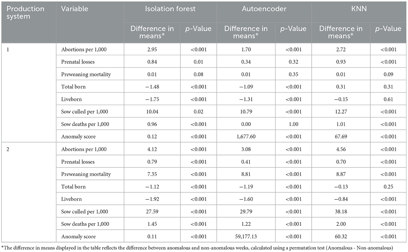
Table 2. Permutation test results for production system 1 and production system 2.

When analyzing the weeks classified as having PRRSV, we see significant differences in many productivity indicators. The abortions per 1,000 sows showed differences across all models, with a large difference in means, particularly in Isolation Forest (3.90, p-value <0.001), followed by KNN (3.91, p-value <0.001), indicating an increase in abortions in anomalous weeks. Significant differences were also observed in total born across all models (p-value <0.01) and liveborn for Isolation Forest and Autoencoder (p-value <0.001), with negative differences suggesting lower numbers in anomalous weeks. Sows culled per 1,000 sows showed an increase in the number of culled sows during anomalous weeks, particularly with the KNN model (15.38, p-value = 0.01). Anomaly scores demonstrated high values in anomalous weeks associated with PRRSV, especially in the Autoencoder model (2,274.80). The weeks classified as “Others” showed less drastic differences in most variables, but sows culled per 1,000 sows and anomaly scores remained significant across all models with p-values <0.001 (Table 3).

Table 3

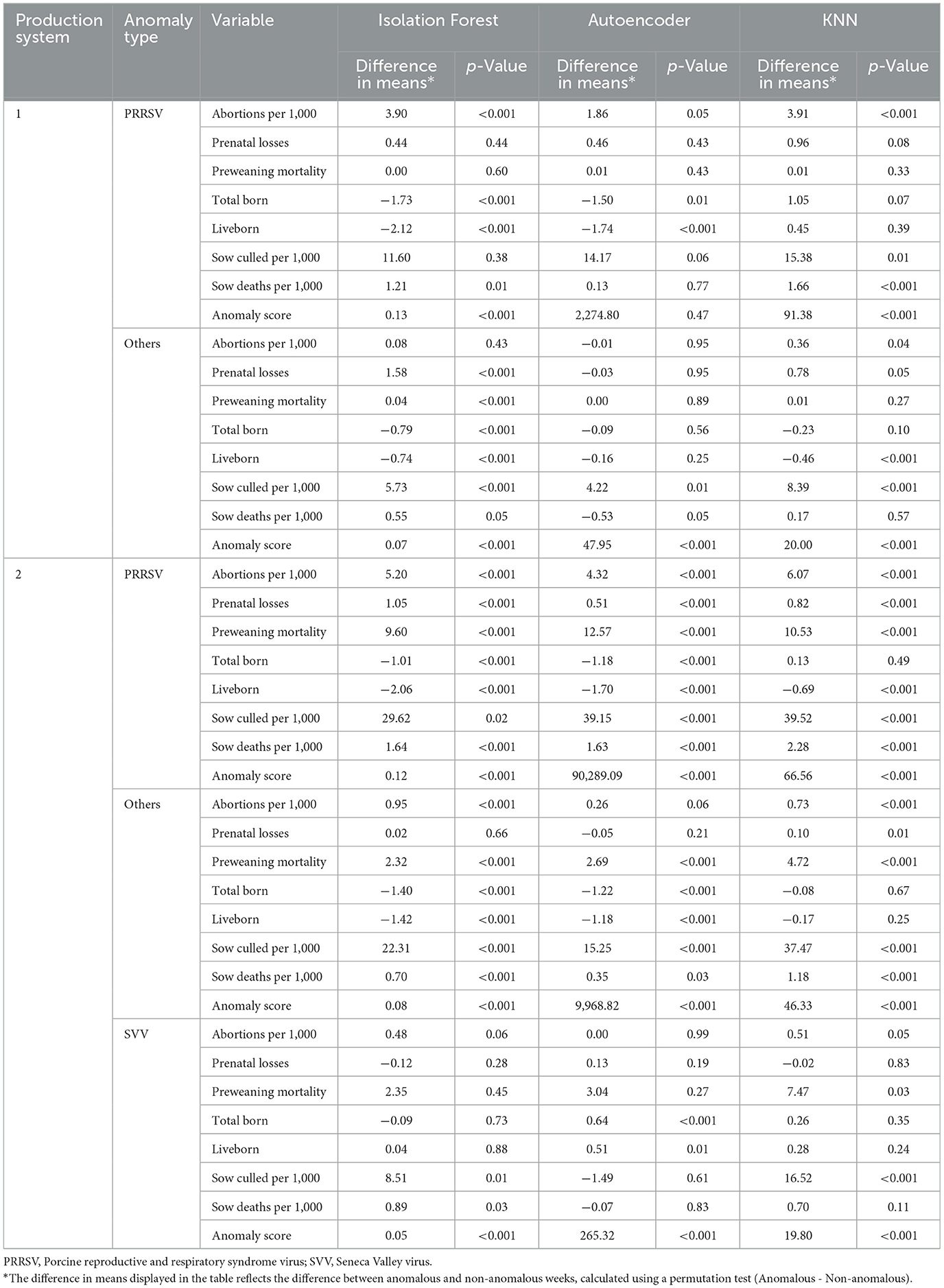
Table 3. Permutation test results for production system 1 and production system 2 for different anomalies.

Based on the density plots for Isolation Forest (Figure 1), Autoencoders (Figure 2), and KNN (Figure 3), it can be concluded that, overall, productivity indicators such as abortions per 1,000 sows and sows culled per 1,000 sows during anomalous weeks (marked in red) tend to be higher than those in non-anomalous weeks (marked in blue). This is evident as the tails of the density curve for anomalous weeks stretch far to the right side of the plot for these productivity indicators, indicating higher values. In contrast, for liveborn and total born, the tails of the density curve for anomalous weeks reach far to the left, signifying lower values compared to non-anomalous weeks.

Figure 1

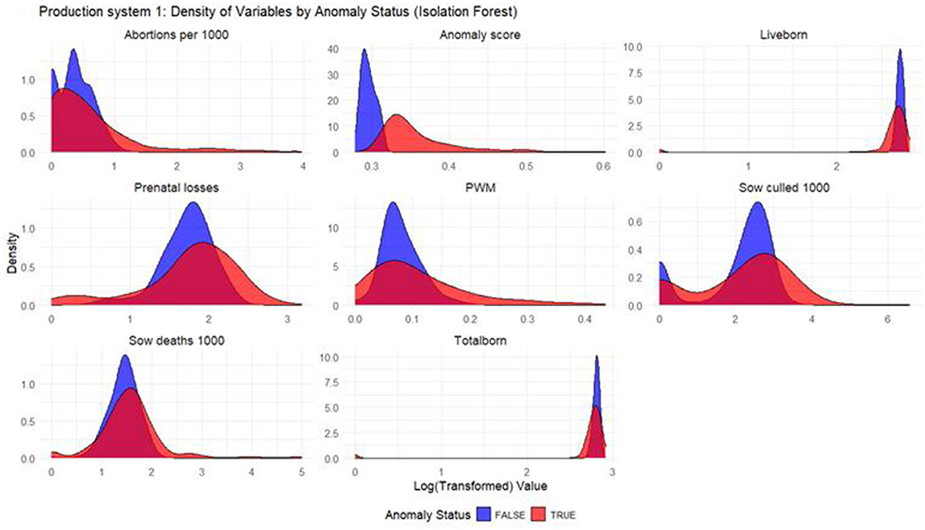
Figure 1. Density plots for Isolation Forest (Production System 1). Each production indicator and the anomaly scores are shown in the density plots; the y-axis represents the density, and the x-axis represents the log value of each variable (the log transformation was done for better interpretation of the chart). The blue color represents the non-anomalous weeks, and the red color represents the anomalous weeks. The plots illustrate how the model separates non-anomalous and anomalous weeks, providing a visual overview of deviations in production indicators relevant for anomaly detection.

Figure 2

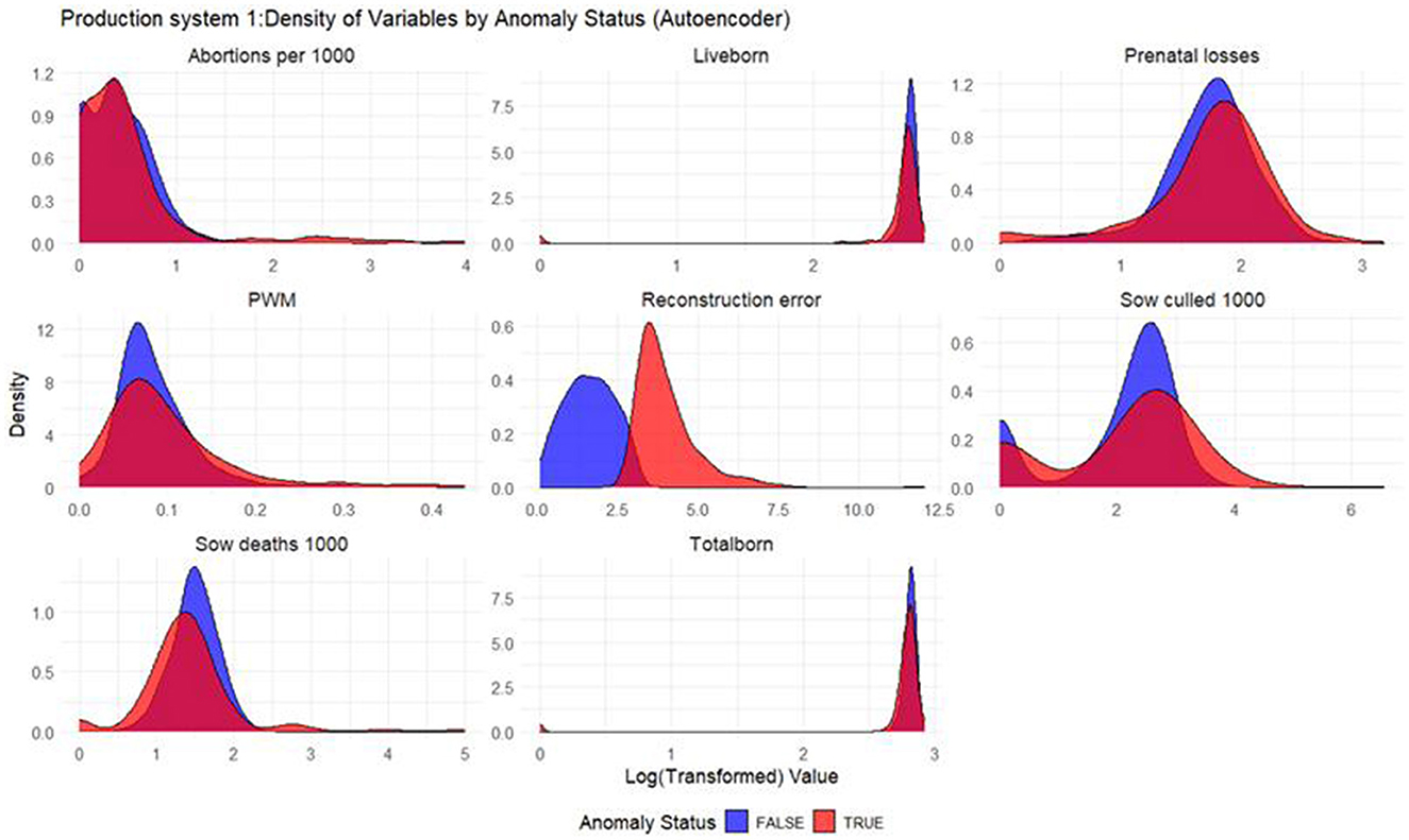
Figure 2. Density plots for Autoencoder (Production System 1). Each production indicator and the reconstruction error are shown in the density plots; the y-axis represents the density, and the x-axis represents the log value of each variable (the log transformation was done for better interpretation of the chart). The blue color represents the non-anomalous weeks, and the red color represents the anomalous weeks. The plots illustrate how the model separates non-anomalous and anomalous weeks, providing a visual overview of deviations in production indicators relevant for anomaly detection.

Figure 3

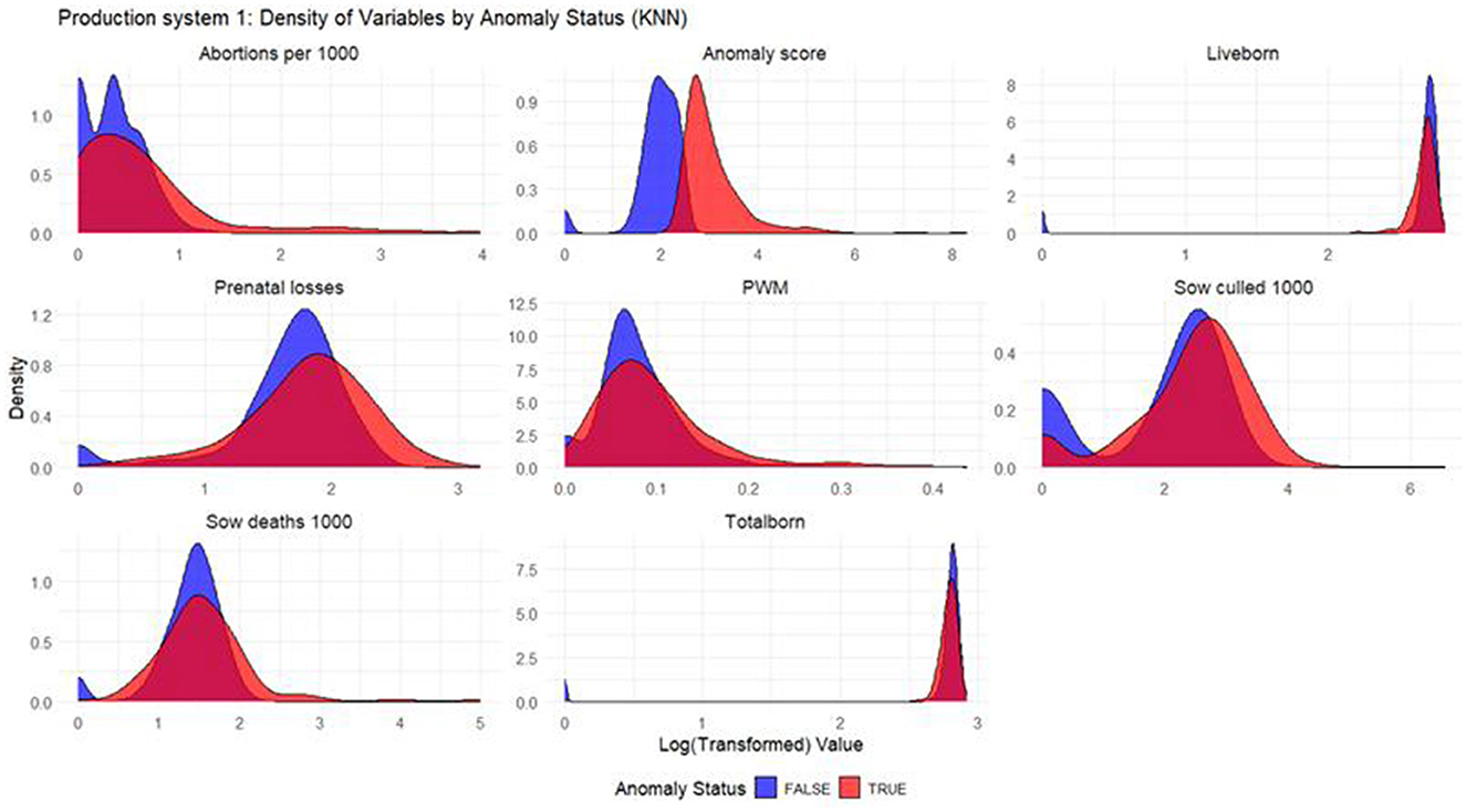
Figure 3. Density plots for KNN (Production System 1). Each production indicator and the anomaly score are shown in the density plots; the y-axis represents the density, and the x-axis represents the log value of each variable (the log transformation was done for better interpretation of the chart). The blue color represents the non-anomalous weeks, and the red color represents the anomalous weeks. The plots illustrate how the model separates non-anomalous and anomalous weeks, providing a visual overview of deviations in production indicators relevant for anomaly detection.

Production System 2

In Production System 2, the differences between anomalous and non-anomalous weeks remain consistent across the three models. Abortions per 1,000 sows showed significant increases for anomalous weeks, with the difference in means ranging from 3.08 (Autoencoder) to 4.56 (KNN), with p-values <0.001. Prenatal losses showed smaller but significant differences across all methods, with Isolation Forest reporting the highest effect (0.79, p-value <0.001). Like Production System 1, total born and liveborn both showed negative differences, with total born decreasing by as much as −1.12, with p-value <0.001 (Isolation Forest), indicating reduced birth rates for anomalous weeks. Sows culled per 1,000 sows showed large differences between anomalous and non-anomalous weeks, with values ranging from 27.59 (Isolation Forest) to 38.18 (KNN), with p-value <0.001, suggesting increased sow culling in this production system during anomalous weeks. The anomaly scores showed a disparity between anomalous and non-anomalous weeks, with Autoencoder reporting a high difference of 59,177.13 with a p-value <0.001 (Table 2).

For the weeks classified as PRRSV, these exhibited significant differences, particularly in abortions per 1,000 sows, which showed differences in means across models (ranging from 4.32 for Autoencoder to 6.07 for KNN, with p-value <0.001), indicating a high number of abortions in anomalous weeks associated with a PRRSV. Similarly, PWM showed significant differences, with high values in anomalous weeks across models (p-value <0.001). Sows culled per 1,000 sows showed high differences in the number of culled sows, particularly with the KNN model (39.52, p-value <0.001). Significant differences in anomaly scores were observed across all models, with extremely high values for PRRSV anomalies, especially in the Autoencoder model (90,289.09, p-value <0.001). The weeks classified as SVV presented more variability, with less consistent differences, particularly in prenatal losses and liveborn. This likely reflects the milder and short-lived clinical expression of SVV in sows, as infection typically resolves within 8–10 days and does not severely affect reproductive parameters, unlike PRRSV (27). However, sows culled 1,000 sows still showed significant differences, with large values for the KNN model (16.52, p-value <0.001). When comparing the weeks classified as “Others,” significant differences in variables like abortions per 1,000 sows (Isolation Forest: 0.95, p-value <0.001; Autoencoder: 0.26, p-value = 0.06; KNN: 0.73, p-value <0.001 ) and sows culled per 1,000 sows (Isolation Forest: 22.31, p-value <0.001; Autoencoder: 15.25, p-value <0.001; KNN: 37.47, p-value <0.001 ) were observed, but with smaller values than those associated with PRRSV (Table 3).

Based on the density plots for Isolation Forest (Figure 4), Autoencoders (Figure 5), and KNN (Figure 6), the conclusions from the charts are like those for Production System 1.

Figure 4

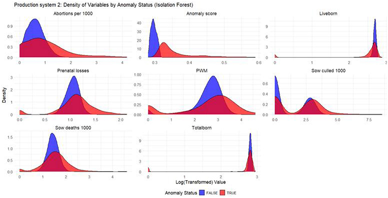
Figure 4. Density plots for Isolation Forest (Production System 2). Each production indicator and the anomaly scores are shown in the density plots; the y-axis represents the density, and the x-axis represents the log value of each variable (the log transformation was done for better interpretation of the chart). The blue color represents the non-anomalous weeks, and the red color represents the anomalous weeks.

Figure 5

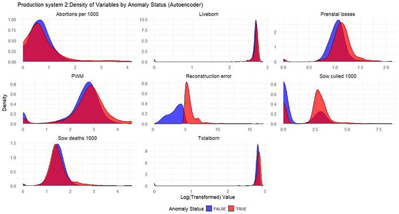
Figure 5. Density plots for Autoencoder (Production System 2). Each production indicator and the reconstruction error are shown in the density plots; the y-axis represents the density, and the x-axis represents the log value of each variable (the log transformation was done for better interpretation of the chart). The blue color represents the non-anomalous weeks, and the red color represents the anomalous weeks.

Figure 6

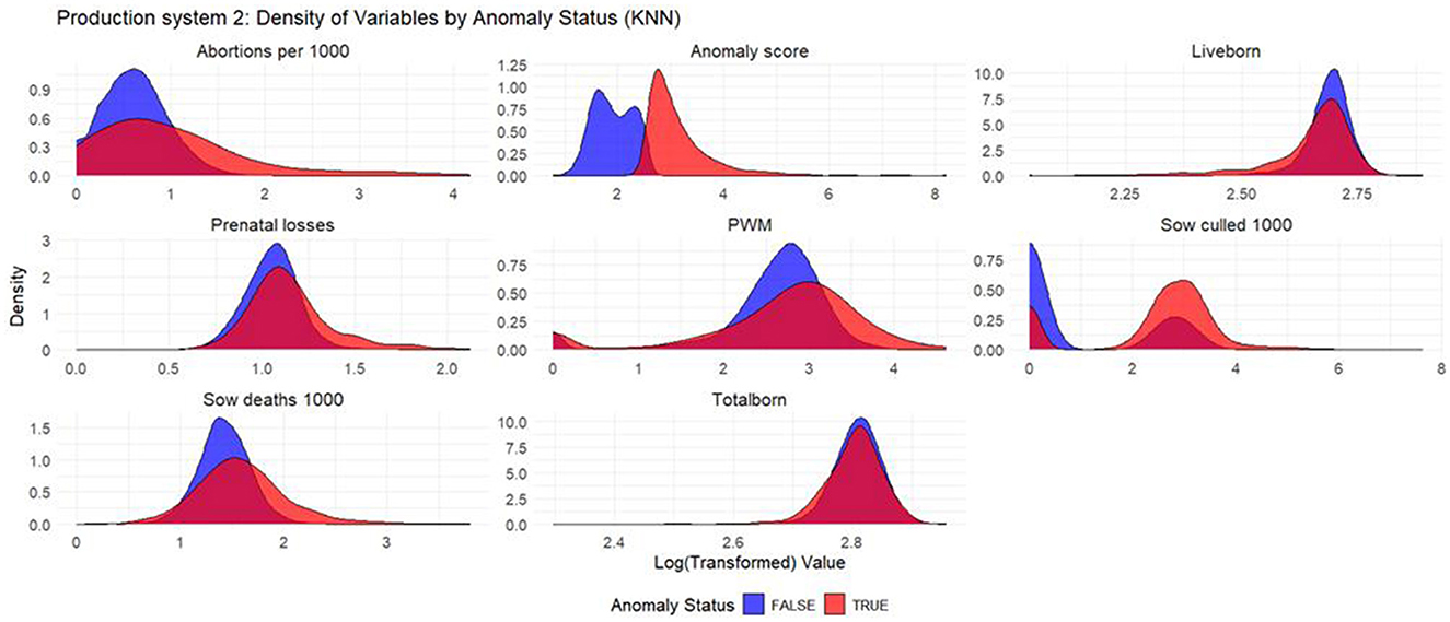
Figure 6. Density plots for KNN (Production System 2). Each production indicator and the anomaly score are shown in the density plots; the y-axis represents the density, and the x-axis represents the log value of each variable (the log transformation was done for better interpretation of the chart). The blue color represents the non-anomalous weeks, and the red color represents the anomalous weeks.

Performance

The models performed well in detecting the PRRSV anomaly, achieving perfect precision (100%) across all methods and for both production systems, with F1-scores ranging from 60% (Autoencoder for Production System 2) to 77% (Isolation Forest for Production System 2). For anomalies like SVV the models showed lower F1-scores for the Isolation Forest and the Autoencoder models compared to PRRSV (Table 4).

Table 4

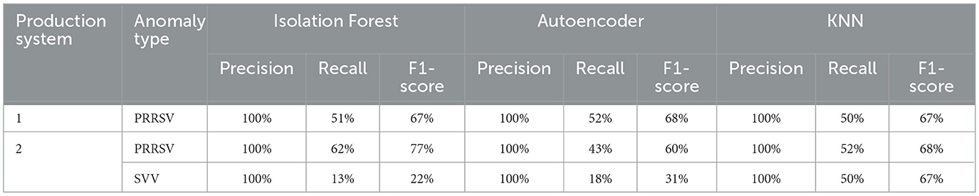
Table 4. Performance metrics per anomaly type for each production system.

PRRSV example line plots

The PRRSV line plots (Figure 7) illustrate the differences between weeks classified as anomalous due to a PRRSV outbreak and those that were not considered anomalous. It can be observed that the number of abortions per 1,000 sows began to rise before the diagnosis of the PRRSV outbreak, especially noticeable in the line plot for Production System 2, and that the number of abortions reached higher values than those reached during the non-anomalous weeks.

Figure 7

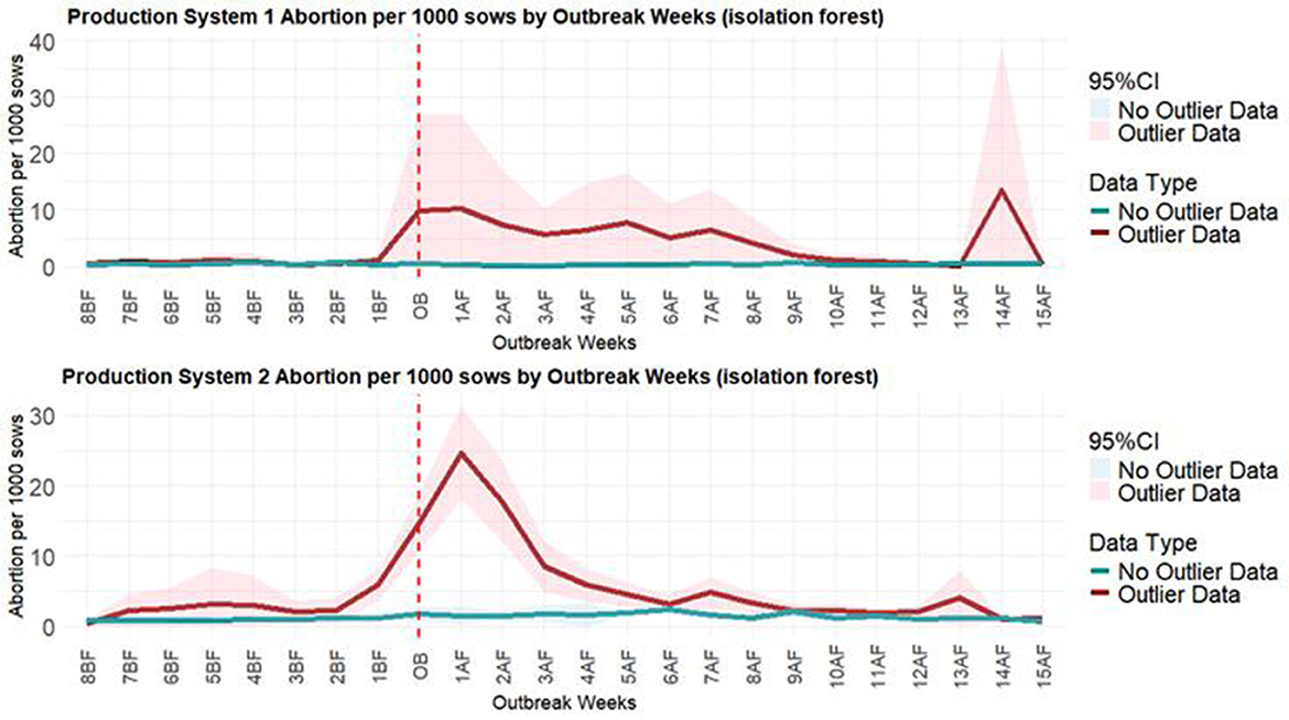
Figure 7. The average of abortions per 1,000 sows in the weeks prior to and following PRRSV outbreaks. The chart on the top refers to the isolation forest model with the average of abortions per 1,000 sows for Production System 1. The chart on the bottom refers to the isolation forest model with the average of abortions per 1,000 sows for Production System 2. The red line is the average for anomalous weeks, and the green line is the average for non-anomalous weeks. The vertical dots refer to the week of the PRRSV outbreak.

Discussion

This paper evaluates the use of unsupervised machine learning models to detect anomalies in productivity indicators on swine farms. Given the increasing automation in data collection and analysis in modern swine production systems, leveraging this data is crucial for monitoring health status and improving farm management (43, 44). These systems collect large volumes of data on production performance, which could be analyzed to identify health-related anomalies. Anomaly detection techniques, such as those explored in this study, can provide early warnings for diseases, enabling timely interventions and enhancing productivity monitoring.

Previous research has explored anomaly detection in the context of animal health and health challenges. For example, gated recurrent units -Autoencoders have been used to detect early signs of respiratory diseases in growing-pig farms, focusing on environmental factors (57). Additionally, a study by (author?) (58) found that the long short-term memory Autoencoder model outperformed other models, including Farrington, Early Aberration Reporting System, and regression models, in detecting anomalies related to PRRSV. Similarly, the Isolation Forest model, previously used to detect estrus in dairy cows (59) and to identify anomalies in temperature and humidity data (60), performed well in distinguishing between anomalous and non-anomalous weeks. The KNN model, known for its effectiveness in both supervised and unsupervised learning (61, 62), showed similar results to the Autoencoder and Isolation Forest models in this study, with anomalous weeks showing significant differences between anomalous and non-anomalous weeks (Table 2).

The models employed in this study represent distinct anomaly detection approaches, each with its strengths and limitations. Isolation Forest is known for its efficiency, scalability, and ability to detect anomalies without assumptions about data distribution, making it suitable for high-dimensional data (28, 29). However, its performance may decline with highly imbalanced datasets or when anomalies closely resemble normal instances (45). In contrast, Autoencoders use neural networks to capture complex, non-linear relationships within high-dimensional datasets, making them effective for detecting subtle anomalies (22). However, they can be computationally intensive and require careful tuning to avoid issues related to training anomalies and generalization (45). KNN, a non-parametric model that requires minimal parameters, is versatile for both classification and regression tasks. However, it struggles with high-dimensional data and is prone to overfitting (46). Despite these limitations, all models provided valuable insights into production behavior during anomalous and non-anomalous weeks (Table 2).

In the case of disease detection, it is of the utmost importance to guarantee that possible epidemics are caught early. Previous studies using statistical process control charts observed that deviations in productivity indicators start to be noticed on average 4 weeks before the diagnostic confirmation of a PRRSV outbreak (8, 10). The results from this study showed that the Isolation Forest, KNN, and Autoencoder models indicated a trend of increasing number of anomalies in productivity indicators associated with outbreaks compared to weeks that were not considered anomalies (Table 3). These findings underscore the complementary nature of the Isolation Forest, KNN, and Autoencoder models, providing valuable insights into how productivity indicators fluctuate during significant events and demonstrating their potential for monitoring and detecting anomalies in swine production systems. For instance, for both production systems, the KNN model detected a higher difference in abortions per 1,000 sows during PRRSV outbreaks (Production System 1: 3.91, Production System 2: 6.07) than the other two models. Conversely, for SVV outbreaks, less pronounced differences between anomalous and non-anomalous weeks were observed across the models, suggesting that SVV-related disruptions may cause less noticeable changes in production performance. These findings underscore the value of applying multiple anomaly detection models to capture a wide range of disease-related fluctuations in swine production. Each model may be sensitive to different types of anomalies, some may detect extreme deviations, while others may better identify subtler or multivariate patterns, so comparing results across models can help uncover patterns that might be missed by any single method (47). Although no formal ensemble or voting approach was tested in this study, evaluating multiple models in parallel provided complementary insights and highlighted the potential for integrating diverse anomaly detection approaches in future work, particularly when routine diagnostics are not implemented at the farm.

The analysis of anomalous and non-anomalous weeks, based on different anomaly classifications (PRRSV, SVV, and Others), reveals variations in the productivity indicators, which aligns with findings from several studies on swine production. For instance, PRRSV-infected herds have been reported to exhibit higher rates of abortion, prenatal loss, and mortality (48, 49), which is consistent with the higher differences in anomaly scores, reconstruction errors, and productivity indicators observed during anomalous weeks in this study (Table 3). Specifically, the increased anomalies in PRRSV-classified weeks suggest a disruption in normal reproductive performance, as demonstrated by the elevated production losses seen in the literature (23). Furthermore, similar trends were observed for SVV, where anomalous weeks showed deviations in productivity indicators, similar to the experimental findings of other studies (24, 50), who reported production losses following SVV infections. These findings also corroborate (26), who emphasized the need for greater surveillance of SVV due to its potential to cause significant production losses. In contrast, non-anomalous weeks, particularly those classified as “Others,” showed smaller differences in productivity indicators between anomalous and non-anomalous weeks (Table 3), reflecting the absence of major health challenges as noted in the literature for non-endemic diseases (48). Collectively, these results highlight the significant role that diseases play in negatively affecting the performance and overall health of swine herds, reinforcing the importance of targeted interventions for mitigating these viral infections.

The F1-score, precision and recall metrics were used to evaluate the performance of the unsupervised anomaly detection models tested in this study (7, 51, 52). These metrics yielded F1-Scores values below 80%, with PRRSV reaching higher performance scores than SVV. As observed by the results of the permutation tests, this was expected, since PRRSV showed a larger difference in means between anomalous and non-anomalous weeks than the SVV and “Others.” It should be taken into consideration that the performance metrics were calculated based on a limited set of labeled data, with only weeks associated with specific health challenges (PRRSV and SVV) considered as true anomalies. In the context of unsupervised learning, these models are particularly useful for exploring patterns in datasets where labeled anomalies are limited. By detecting deviations without relying solely on predefined labels, the models in this study were able to highlight weeks with statistically significant differences from non-anomalous weeks, as confirmed by permutation tests comparing productivity indicators. This suggests that unsupervised approaches can help reveal anomalies that may have been missed, undiagnosed, or mislabeled, providing insight into potentially overlooked issues within the production system. While supervised models depend on the availability and accuracy of labels, unsupervised models can flag unusual patterns even when diagnostic data are incomplete or uncertain. One practical way to leverage these insights is through the creation of production scores that summarize deviations across production systems or farms. For example, farms or production systems could be categorized based on overall performance scores derived from anomaly detection outputs, allowing managers to identify areas with major deviations and prioritize investigations. Such scoring frameworks can provide a structured and interpretable method to monitor production variability.

While this study provides valuable insights into anomaly detection for disease monitoring in swine farms, it is important to acknowledge its limitations. The analysis primarily focused on health challenges, particularly PRRSV and SVV, and did not consider other factors that may influence the appearance of anomalies, such as environmental conditions or management practices. These models are intended to be agnostic, that is, they flag deviations in productivity indicators without assuming a specific cause, serving as an exploratory tool to highlight potential issues rather than a definitive measure of disease presence. Some flagged anomalies may represent false positives, triggered by routine management activities (e.g., vaccination, moving sows, or issues with electronic sow feeders), environmental events (e.g., weather), or missing data inputs, while others could reflect undiagnosed or emerging health challenges. if data are not entered or if key variables show unexpected gaps, the models would likely identify this as an anomaly, since the resulting deviation from the established farm-specific pattern differs from the expected trajectory of production indicators. In this sense, the models can also serve as a tool to detect irregularities in data recording or reporting practices. However, they cannot distinguish between anomalies arising from biological events and those caused by data-entry errors, emphasizing the need for human interpretation of the alerts. In this study, a threshold using the 75th percentile was used, but thresholds may need to be tuned in each production system to balance sensitivity and specificity, for example, by adjusting cutoffs based on production system-specific baseline variability or by applying adaptive approaches that account for temporal changes. Furthermore, the study did not assess PRRSV statuses prior to outbreak reports, which could have impacted the results, as farms with different levels of prior exposure to PRRSV may exhibit varying responses. Another potential limitation of the data used in this study is that the data for the same herds across consecutive weeks may exhibit temporal correlation. For example, production indicators could be influenced by health or environmental factors persisting over time. However, the models used in this study focus on detecting local anomalies based on deviations from the learned distribution or neighborhood (53). These models are not explicitly designed to account for temporal correlations but are still effective at identifying significant deviations regardless of the relationship between weeks.

Future research could broaden the scope by considering additional factors like environmental conditions, pathogen introductions, or farm management differences, providing a more comprehensive understanding of anomaly detection in swine production systems. Moreover, exploring other farm settings, such as nurseries or wean-to-finish operations, could offer further insights into the robustness and applicability of the models tested in this study. Additionally, considering the incorporation of time-series models or temporal correlation-aware anomaly detection techniques could be used to capture the dependencies of production indicators over time and enhance the model performance (54).

Conclusion

The utility of unsupervised machine learning techniques in detecting anomalies was demonstrated in this study, paving the way for more proactive management strategies in livestock health. By employing Isolation Forest, Autoencoder, and KNN models, it was found that anomalous weeks showed a significant difference in the overall values of the productivity indicators, anomaly scores, and reconstruction errors compared to non-anomalous weeks. These findings highlight the potential for using productivity indicators to aid decision-makers in implementing surveillance systems, mainly in farms that are not routinely collecting samples for diagnostics. Monitoring these data is crucial for triggering timely diagnostic tests and treatments and enhancing biosecurity measures, ultimately contributing to improved animal welfare and farm productivity during health challenges.

Data availability statement

The data that support the findings of this study belong to two production systems and restrictions apply to the availability of these data, which were used under license for the current study, and so are not publicly available. Data are, however, available from the authors upon reasonable request and with permission of the production systems. Requests to access the datasets should be directed to Z3VzdGF2b3NAaWFzdGF0ZS5lZHU=.

Author contributions

MP: Conceptualization, Formal analysis, Funding acquisition, Investigation, Methodology, Software, Validation, Visualization, Writing – original draft, Writing – review & editing. CW: Methodology, Supervision, Validation, Writing – original draft, Writing – review & editing. GT: Writing – original draft, Writing – review & editing. FD: Writing – original draft, Writing – review & editing. DL: Writing – original draft, Writing – review & editing. DH: Writing – original draft, Writing – review & editing. GS: Conceptualization, Methodology, Supervision, Writing – original draft, Writing – review & editing.

Funding

The author(s) declare that financial support was received for the research and/or publication of this article. This study was funded by the U.S. Department of Agriculture -National Institute of Food and Agriculture (USDA-NIFA) #2023-68008-39860.

Acknowledgments

The authors thank the production systems for collaborating in the study by providing the production and diagnostic data used in the analyses.

Conflict of interest

The authors declare that the research was conducted in the absence of any commercial or financial relationships that could be construed as a potential conflict of interest.

The reviewer DM declared a past co-authorship with the author(s) GT, DCLL, DH to the handling editor.

Generative AI statement

The author(s) declare that Gen AI was used in the creation of this manuscript. Generative AI (Grammarly and GPT-4o-mini model) was used to correct English mistakes and sentence writing.

Any alternative text (alt text) provided alongside figures in this article has been generated by Frontiers with the support of artificial intelligence and reasonable efforts have been made to ensure accuracy, including review by the authors wherever possible. If you identify any issues, please contact us.

Publisher's note

All claims expressed in this article are solely those of the authors and do not necessarily represent those of their affiliated organizations, or those of the publisher, the editors and the reviewers. Any product that may be evaluated in this article, or claim that may be made by its manufacturer, is not guaranteed or endorsed by the publisher.

References

1. Osemeke OH, Souza e Silva G, Corzo C, Kikuti M, Yue X, Linhares DCL, et al. Updating the Productivity and Economic Costs of PRRSV in the US. Oral Presentation. Liepzig, Germany: International Pig Society Congress (2024). Available online at: https://storage.mzevents.it/Programme_IPVSandESPHM2024.pdf (Accessed January 15, 2025).

Google Scholar

2. Nieuwenhuis N, Duinhof TF, van Nes A. Economic analysis of outbreaks of porcine reproductive and respiratory syndrome virus in nine sow herds. Vet Rec. (2012) 170:225. doi: 10.1136/vr.100101

PubMed Abstract | Crossref Full Text | Google Scholar

3. Stevenson GW, Hoang H, Schwartz KJ, Burrough ER, Sun D, Madson D, et al. Emergence of porcine epidemic diarrhea virus in the United States: clinical signs, lesions, and viral genomic sequences. J Vet Diagn Investig. (2013) 25:649–54. doi: 10.1177/1040638713501675

PubMed Abstract | Crossref Full Text | Google Scholar

4. Weng L, Weersink A, Poljak Z, de Lange K, von Massow M. An economic evaluation of intervention strategies for porcine epidemic diarrhea (PED). Prev Vet Med. (2016) 134:58–68. doi: 10.1016/j.prevetmed.2016.09.018

PubMed Abstract | Crossref Full Text | Google Scholar

5. Stancu A. ASF evolution and its economic impact in europe over the past decade. USV Ann Econ Publ Adm. (2018) 18:18–27. doi: 10.4316/aepa.2018.18.2(28).18-27

Crossref Full Text | Google Scholar

6. Carriquiry M, Elobeid A, Swenson DA, Hayes DJ. Impacts of African Swine Fever in Iowa and the United States. Center for Agricultural and Rural Development (CARD) Publications (2020). March, 20-wp600. Available online at: https://ideas.repec.org//p/ias/cpaper/20-wp600.html (Accessed January 15, 2025).

Google Scholar

7. Shriram S, Sivasankar E. Anomaly Detection on Shuttle Data Using Unsupervised Learning Techniques. 2019 International Conference on Computational Intelligence and Knowledge Economy (ICCIKE) (2019). p. 221–25. doi: 10.1109/ICCIKE47802.2019.9004325

Crossref Full Text | Google Scholar

8. Silva GS, Schwartz M, Morrison RB, Linhares DCL. Monitoring breeding herd production data to detect PRRSV outbreaks. Prev Vet Med. (2017) 148:89–93. doi: 10.1016/j.prevetmed.2017.10.012

PubMed Abstract | Crossref Full Text | Google Scholar

9. Merca C, Lindell IC, Ernholm L, Selling LE, Nunes TP, Sjölund M, et al. Veterinary syndromic surveillance using swine production data for farm health management and early disease detection. Prev Vet Med. (2022) 205:105659. doi: 10.1016/j.prevetmed.2022.105659

PubMed Abstract | Crossref Full Text | Google Scholar

10. Pedro Mil-Homens M, Jayaraman S, Rupasinghe K, Wang C, Trevisan G, Dórea F, et al. Early detection of PRRSV outbreaks in breeding herds by monitoring productivity and electronic sow feed data using univariate and multivariate statistical process control methods. Transbound Emerg Dis. (2024) 2024:9984148. doi: 10.1155/2024/9984148

PubMed Abstract | Crossref Full Text | Google Scholar

11. Allard R. Use of time-series analysis in infectious disease surveillance. Bullet World Health Organ. (1998) 76:327–33.

PubMed Abstract | Google Scholar

12. Blázquez-García A, Conde A, Mori U, Lozano JA. A review on outlier/anomaly detection in time series data. ACM Comput Surv. (2022) 54:1–33. doi: 10.1145/3444690

Crossref Full Text | Google Scholar

13. Caruana R, Niculescu-Mizil A. An Empirical Comparison of Supervised Learning Algorithms. Proceedings of the 23rd International Conference on Machine Learning - ICML '06 (2006). p. 161–68. doi: 10.1145/1143844.1143865

Crossref Full Text | Google Scholar

14. Amruthnath N, Gupta T. A Research Study on Unsupervised Machine Learning Algorithms for Early Fault Detection in Predictive Maintenance. 2018 5th International Conference on Industrial Engineering and Applications (ICIEA) (2018). p. 355–61. doi: 10.1109/IEA.2018.8387124

Crossref Full Text | Google Scholar

15. Eskin E, Arnold A, Prerau M, Portnoy L, Stolfo S. (2002) A geometric framework for unsupervised anomaly detection. In:Barbará D, Sushil J, , editors. Applications of Data Mining in Computer Security. Advances in Information Security. Springer US. p. 77–101. doi: 10.1007/978-1-4615-0953-0_4

Crossref Full Text | Google Scholar

16. Xu J, Zhou S, Xia F, Xu A, Ye J. Research on the lying pattern of grouped pigs using unsupervised clustering and deep learning. Livest Sci. (2022) 260:104946. doi: 10.1016/j.livsci.2022.104946

Crossref Full Text | Google Scholar

17. Barbosa L, Lopes PS, Regazzi AJ, Guimarães SEF, Torres RA. Identification of informative performance traits in swine using principal component analysis. Arq Bras Med Vet Zootec. (2005) 57:805–10. doi: 10.1590/S0102-09352005000600016

Crossref Full Text | Google Scholar

18. Buzzard L, Smith S, Dixon A, Kenny J, Appleman M, Subramanian S, et al. Principal component analysis of a swine injury model identifies multiple phenotypes in trauma. J Trauma Acute Care Surg. (2024) 96:634. doi: 10.1097/TA.0000000000004098

PubMed Abstract | Crossref Full Text | Google Scholar

19. Baron JN, Aznar MN, Monterubbianesi M, Martínez-López B. Application of network analysis and cluster analysis for better prevention and control of swine diseases in Argentina. PLoS ONE. (2020) 15:e0234489. doi: 10.1371/journal.pone.0234489

PubMed Abstract | Crossref Full Text | Google Scholar

20. Ahmad S, Lavin A, Purdy S, Agha Z. Unsupervised real-time anomaly detection for streaming data. Neurocomputing. (2017) 262:134–47. doi: 10.1016/j.neucom.2017.04.070

Crossref Full Text | Google Scholar

21. Zhong S, Fu S, Lin L, Fu X, Cui Z, Wang R. A Novel Unsupervised Anomaly Detection for Gas Turbine Using Isolation Forest. 2019 IEEE International Conference on Prognostics and Health Management (ICPHM) (2019). p. 1–6. doi: 10.1109/ICPHM.2019.8819409

Crossref Full Text | Google Scholar

22. Cheng Z, Wang S, Zhang P, Wang S, Liu X, Zhu E. Improved autoencoder for unsupervised anomaly detection. Int J Intell Syst. (2021) 36:7103–25. doi: 10.1002/int.22582

Crossref Full Text | Google Scholar

23. Baysinger AK, Dewey CE, Straw BE, Brumm MC, Schmitz J, Doster A, et al. The effect of PRRSV on reproductive parameters in swine herds. J Swine Health Produc. (1997) 5:173–76. Available online at: https://www.aasv.org/shap/issues/v5n5/v5n5p173.pdf

Google Scholar

24. Kim H, Buckley A, Guo B, Kulshreshtha V, Geelen AV, Montiel N, et al. Experimental seneca valley virus infection in sows and their offspring. Vet Microbiol. (2024) 289:109958. doi: 10.1016/j.vetmic.2023.109958

PubMed Abstract | Crossref Full Text | Google Scholar

25. Zimmerman J, Karriker L, Ramirez A, Schwartz K, Stevenson G, Zhang J. Diseases of Swine. 11th ed. Hoboken, NJ: Wiley-Blackwell (2019). doi: 10.1002/9781119350927

Crossref Full Text | Google Scholar

26. Zhang X, Zhu Z, Yang F, Cao W, Tian H, Zhang K, et al. Review of seneca valley virus: a call for increased surveillance and research. Front Microbiol. (2018) 9:940. doi: 10.3389/fmicb.2018.00940

PubMed Abstract | Crossref Full Text | Google Scholar

27. Senecavirus A Iowa State University (2024). Iowa state university college of veterinary medicine, Veterinary diagnostic laboratory. Available online at: https://vetmed.iastate.edu/vdl/resources/client-services/pathogens/senecavirus (Accessed November 22, 2024).

Google Scholar

28. Liu FT, Ting KM, Zhou Z.-H. Isolation Forest. 2008 Eighth IEEE International Conference on Data Mining (2008). p. 413–22. doi: 10.1109/ICDM.2008.17

Crossref Full Text | Google Scholar

29. Al Farizi WS, Hidayah I, Nur Rizal M. Isolation Forest Based Anomaly Detection: A Systematic Literature Review. 2021 8th International Conference on Information Technology, Computer and Electrical Engineering (ICITACEE) (2021). p. 118–22. doi: 10.1109/ICITACEE53184.2021.9617498

Crossref Full Text | Google Scholar

30. Kuhn M. Building predictive models in R using the caret package. J Stat Softw. (2008) 28:1–26. doi: 10.18637/jss.v028.i05

Crossref Full Text | Google Scholar

31. Wickham H, Henry L. Purrr: Functional Programming Tools. R Package Version 1.0.2 (2023). Available online at: https://github.com/tidyverse/purrr (Accessed November 12, 2024).

Google Scholar

32. Cortes D. Isotree: Isolation-Based Outlier Detection Version 0.6.1-1 (2024). Available online at: https://cran.r-project.org/web/packages/isotree/index.html (Accessed November 12, 2024).

Google Scholar

33. Chandola V, Banerjee A, Kumar V. Anomaly detection: a survey. ACM Comput Surv. (2009) 41:1–58. doi: 10.1145/1541880.1541882

Crossref Full Text | Google Scholar

34. Balabit Unsupervised. Novel Performance Metrics for Anomaly Detection Algorithms. Balabit Unsupervised (2018). Available online at: https://medium.com/data-science/isolation-forest-with-statistical-rules-4dd27dad2da9 (Accessed January 24, 2025).

Google Scholar

35. Krishnan A. Isolation Forest with Statistical Rules. Medium towards Data Science (2019). Available online at: https://towardsdatascience.com/isolation-forest-with-statistical-rules-4dd27dad2da9 (Accessed January 24, 2025).

Google Scholar

36. H2O.ai (2024). H2O.Ai. Isolation Forest 3.46.0.6. Available online at: https://docs.h2o.ai/h2o/latest-stable/h2o-docs/data-science/if.html (Accessed January 24, 2025).

Google Scholar

37. Ryckel F. Chapter 7 KNN - K Nearest Neighbour | Machine Learning with R (2024). Available online at: https://fderyckel.github.io/machinelearningwithr/knnchapter.html (Accessed November 11, 2025).

Google Scholar

38. Yi J, Yoon S. CKNN: Cleansed k-Nearest Neighbor for Unsupervised Video Anomaly Detection. Proceedings of the 33rd ACM International Conference on Information and Knowledge Management (New York, NY, USA), CIKM '24 (2024). p. 3002–11. doi: 10.1145/3627673.3679526

Crossref Full Text | Google Scholar

39. Schliep K, Hechenbinchler K, Lizee A. Weighted K-Nearest Neighbors, Version 1.3.1 (2016). Available online at: https://cran.r-project.org/web/packages/kknn/kknn.pdf (Accessed November 12, 2024).

Google Scholar

40. Li S. FNN: Fast Nearest Neighbor Search Algorithms and Applications, Version 1.1.4.1 (2024). Available online at: https://cran.r-project.org/web/packages/FNN/index.html (Accessed November 12, 2024).

Google Scholar

41. Fryda T. H2o: R Interface for the ‘H2O' Scalable Machine Learning Platform, Version 3.44.0.3 (2024). Available online at: https://cran.r-project.org/web/packages/h2o/index.html (Accessed November 12, 2024).

Google Scholar

42. Good P. Permutation Tests. Springer Series in Statistics. New York, NY: Springer (2000). doi: 10.1007/978-1-4757-3235-1_14

Crossref Full Text | Google Scholar

43. Moso JC, Cormier S, de Runz C, Fouchal H, Wandeto JM. Anomaly detection on data streams for smart agriculture. Agriculture. (2021) 11:11. doi: 10.3390/agriculture11111083

Crossref Full Text | Google Scholar

44. Burns RT, Spajić R, Burns RT, Spajić R. Precision livestock farming in swine production. In: Tracing the Domestic Pig. IntechOpen (2024) 1–15. doi: 10.5772/intechopen.114845

Crossref Full Text | Google Scholar

45. Sadaf K, Sultana J. Intrusion detection based on autoencoder and isolation forest in fog computing. IEEE Access. (2020) 8:167059–68. doi: 10.1109/ACCESS.2020.3022855

Crossref Full Text | Google Scholar

46. IBM. What Is the K-Nearest Neighbors Algorithm? | IBM (2021). Available online at: https://www.ibm.com/topics/knn (Accessed January 10, 2025).

Google Scholar

47. Provotar OI, Linder YM, Veres MM. Unsupervised Anomaly Detection in Time Series Using LSTM-Based Autoencoders. 2019 IEEE International Conference on Advanced Trends in Information Theory (ATIT) (2019). p. 513–17. doi: 10.1109/ATIT49449.2019.9030505

Crossref Full Text | Google Scholar

48. Valdes-Donoso P, Alvarez J, Jarvis LS, Morrison RB, Perez AM. Production losses from an endemic animal disease: porcine reproductive and respiratory syndrome (PRRS) in selected Midwest US Sow Farms. Front Vet Sci. (2018) 5:102. doi: 10.3389/fvets.2018.00102

PubMed Abstract | Crossref Full Text | Google Scholar

49. Torrents D, Miranda J, Gauger PC, Ramirez A, Linhares DCL. Effect of PRRSV stability on productive parameters in breeding herds of a swine large integrated group in Spain. Porcine Health Manag. (2021) 7:21. doi: 10.1186/s40813-021-00203-4

PubMed Abstract | Crossref Full Text | Google Scholar

50. Zhang J, Li C, Meng Y, Xie Y, Shi N, Zhang H, et al. Pathogenicity of seneca valley virus in pigs and detection in culicoides from an infected pig farm. Virol J. (2021) 18:209. doi: 10.1186/s12985-021-01679-w

PubMed Abstract | Crossref Full Text | Google Scholar

51. John H, Naaz S. Credit card fraud detection using local outlier factor and isolation forest. Int J Comput Sci Eng. (2019) 7:1060–64. doi: 10.26438/ijcse/v7i4.10601064

Crossref Full Text | Google Scholar

52. Xu W, Jang-Jaccard J, Singh A, Wei Y, Sabrina F. Improving performance of autoencoder-based network anomaly detection on NSL-KDD dataset. IEEE Access. (2021) 9:140136–46. doi: 10.1109/ACCESS.2021.3116612

Crossref Full Text | Google Scholar

53. Hodge V, Austin J. A survey of outlier detection methodologies. Artif Intell Rev. (2004) 22:85–126. doi: 10.1023/B:AIRE.0000045502.10941.a9

Crossref Full Text | Google Scholar

54. Chalapathy R, Chawla S. Deep learning for anomaly detection: a survey. arXiv. (2019) [Preprint].

Google Scholar

55. North American Meat Institute. NAFTA's Positive Impact on U.S. Meat Trade (2016). Available online at: https://www.porgwebnidta.com/ht/a/GetDocumentAction/i/140210.pdf (Accessed February 2025).

Google Scholar

56. R Core Team. R: A Language and Environment for Statistical Computing. Vienna: R Foundation for Statistical Computing (2024). Available online at: https://www.R-project.org/.

Google Scholar

57. Cowton J, Kyriazakis I, Plötz T, Bacardit J. A combined deep learning GRU-Autoencoder for the early detection of respiratory disease in pigs using multiple environmental sensors. Sensors. (2018) 18:2521. doi: 10.3390/s18082521

PubMed Abstract | Crossref Full Text | Google Scholar

58. Díaz-Cao JM, Liu X, Kim J, Clavijo M, Martínez-López B. Evaluation of the application of sequence data to the identification of outbreaks of disease using anomaly detection methods. Vet Res. (2023) 54:75. doi: 10.1186/s13567-023-01197-3

PubMed Abstract | Crossref Full Text | Google Scholar

59. Medema E, Hons B. Bovine Event Detection: Analysis of Bovine Data and Cycles. The University of British Columbia (2022). Available online at: https://open.library.ubc.ca/media/stream/pdf/52966/1.0413675/5 (Accessed October, 2024).

Google Scholar

60. Fahaad Alumfareh M, Humayun M, Ahmad Z, Khan A. An intelligent LoRaWAN-based IoT device for monitoring and control solutions in smart farming through anomaly detection integrated with unsupervised machine learning. IEEE Access. (2024) 12:11907286. doi: 10.1109/ACCESS.2024.3450587

Crossref Full Text | Google Scholar

61. Molares-Ulloa A, Fernandez-Blanco E, Pazos A, Rivero D. Machine learning in management of precautionary closures caused by lipophilic biotoxins. Comput Electron Agric. (2024) 197:106956. doi: 10.1016/j.compag.2022.106956

Crossref Full Text | Google Scholar

62. Pinto e Silva I. Anomaly Detection in Pet Behavioural Data. Faculdade de Economia; Universidade do Porto (2023). Available online at: https://repositorio-aberto.up.pt/bitstream/10216/151287/2/635322.pdf (Accessed November, 2024).

Google Scholar