A Space-Time Study of Hemorrhagic Fever with Renal Syndrome (HFRS) and Its Climatic Associations in Heilongjiang Province, China

Introduction

Hemorrhagic fever with renal syndrome (HFRS) is a rodent-borne zoonosis caused by Hantavirus (belonging to the Bunyaviridae family). In China, the Hantaan and Seoul viruses dominate HFRS infection, the leading rodent hosts of which are Apodemus agrarius and Rattus norvegicus, respectively [1, 2]. The virus is transmitted from rodents to humans via inhalation of aerosols contaminated by rodents' urine, saliva, excreta, and dung, possibly through ingestion of contaminated food and by direct contact of contaminated materials with broken skin or mucous membranes, or by rodent bites [3, 4]. Clinical HFRS manifestations include fever, headache, nausea, and abdominal pain. Complications, like adverse kidney effects and subsequent pulmonary edema, shock, renal insufficiency, encephalopathy, hemorrhages, and cardiac complications, can cause death [5, 6]. The disease goes through five stages: febrile, hypotensive shock, oliguric, polyuric, and convalescent, which last, respectively, 1–7 days, 1–3 days, 2–6 days, 2 weeks, and 3–6 months [7].

Historically, numerous HFRS-like cases have occurred in China going back to the tenth century AD. Currently, about 20,000–50,000 cases/year are reported in mainland China, which account for 90% of all reported cases worldwide [5, 8, 9]. The foci of HFRS often locates in rural areas, which constitute more than 70% of the total number of cases, because of poor housing conditions and abundant rodent hosts [10, 11]. According to the data of the National Health and Family Planning Commission of China, the HFRS death rate was 2.89% during 1950–2014 [7]. Rattus norvegicus, which hosts the Seoul virus, is regarded as one of the most damaging invasive species around the world, and it is closely associated with humans, particularly in large metropolitan areas [12, 13]. As HFRS remains a severe public health problem, it is necessary to study historical HFRS evidence to provide rigorous scientific support to current disease monitoring and control procedures. Yet, so far there exists a very limited number of quantitative studies regarding the spatiotemporal HFRS distribution and spread in Heilongjiang province. In fact, the reason for the development of the present work is to make up the lack of such quantitative studies.

Based on province-level data, a number of nationwide studies have been carried out in China. Their results indicated that the geographical distribution of HFRS incidences was clustered, particularly in the northeastern, central and eastern parts of China. The observed hotspots shifted and expanded from year to year, whereas most HFRS cases were mainly reported during the spring and the autumn-winter seasons [14–16]. In these studies, global indicators of spatial autocorrelation (GISA), local indicators of spatial association (LISA) and Kulldorff's scan statistic were employed to characterize the spatial variation of HFRS incidence during several time periods. However, these studies suffered from certain drawbacks: (a) they considered neither the temporal nor the combined space-time (spatiotemporal) correlation of HFRS incidences, and (b) a fine temporal resolution (i.e., monthly data) was assumed, whereas the spatial resolution used for mapping purposes was rather coarse (i.e., at the province-level).

For more than two decades, the Bayesian Maximum Entropy theory of space-time data analysis and mapping (BME, [17–19]) has been proven to provide efficient and cost-effective methods for characterizing, predicting and mapping disease attributes (such as disease incidence) in a composite space-time domain under conditions of in-situ uncertainty [20]. For example, Law et al. [21] used BME to qualitatively and quantitatively detect core areas with high syphilis incidence density in the city of Baltimore (USA) between the years 1994 and 2002; also, based on age-adjusted influenza mortality data at the county-level, Choi et al. [22] used BME to represent the space-time disease dependence structure of the disease, to map the influenza mortality rates and to assess the associated disease risk in the state of California (USA). In this work, we will use both the original BME and a BME variant (projected BME, P-BME) to study the spatiotemporal HFRS dependence pattern in Heilongjiang province, including the identification of particular disease features and the detection of high incidence areas.

Since HFRS is transmitted by reservoir hosts (especially rodents), it is expected that climatic factors (such as precipitation, temperature, humidity, and global climate pattern) should influence human HFRS morbidity by affecting the reproduction and abundance of rodents [3, 23–27]. To some extent, understanding climate change can offer a preliminarily assessment or an early warning concerning the epidemic situation. Few studies have investigated the intrinsic HFRS period and its inherent relationships with climate attributes and factors. In recent years, the Hilbert–Huang transformation (HHT, an adaptive method combining empirical mode decomposition and spectral analysis) has been developed for analyzing nonlinear and temporally non-stationary data, in general [28–30]. With this method, the intrinsic mode and intensity of a disease attribute is obtained that can provide useful insight regarding the temporal regulation of disease variation. Moreover, cross-wavelet transforms and wavelet coherence can explore the relationship between two series in the time-frequency domain [31]. As a matter of fact, the wavelet method has been employed in the past to study disease incidence and climate change. For example, Thai et al. [32] have found a strong non-stationary association between El Niño-Southern Oscillation (ENSO) indices and climate variables and the corresponding dengue incidence in the Binh Thuan province (Vietnam) during a 2–3 years period; also, Chowell et al. [33] have suggested that in Peru the dengue incidence is significantly linked with the seasonal cycle timing of mean temperature variations.

In view of the above considerations, the objective of this work is two-fold: (1) to investigate the characteristics and spatiotemporal distribution of HFRS incidence in Heilongjiang province (China) using the BME and P-BME methods; and (2) to assess the intrinsic mode and coherence similarities between the HFRS incidence spread and the time series of key climatic factors using the Hilbert-Huang spectrum method and wavelet analysis.

Materials and Methods

Study Area and Data Collection

The Heilongjiang province is located in northeastern China, with an area of ~473,000 Km² and a population of 38.35 million people. Remarkably, the Heilongjiang province is one of the highest HFRS morbidity regions in China [34]. The Heilongjiang basin includes four major river systems: the Heilong, Songhua, Wusuli, and Suifen rivers (Figure 1). Monthly data of HFRS cases (21,383 cases in total) were collected at 130 counties and districts during the January 2005–December 2013 period by the China Information System for Disease Control and Prevention (CISDCP). Demographic data for each county were obtained from the National Bureau of Statistics of China. Subsequently, the HFRS cases were population-standardized and used in the present work.

FIGURE 1

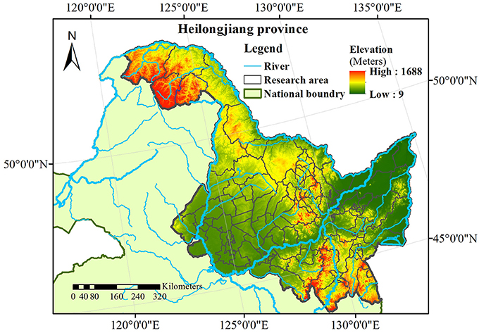
Figure 1. Study area and delimiter of counties and districts.

The multivariate ENSO Index (MEI) integrates 6 oceanic and meteorologic variables over the tropical Pacific region to represent global climatic cycles (i.e., El Niño-Southern Oscillation): sea-level pressure, zonal and meridional components of surface wind, sea surface temperature, surface air temperature, and total cloudiness fraction of sky [35]. The MEI has been used in the scientific literature to diagnose ENSO phenomena that can cause global climate variability, including world-wide correlations with temperature and precipitation data [36]. In the present study, the MEI is employed as a proxy for representing climatic factors in order to explore their effects on HFRS incidence (MEI data is available at https://www.esrl.noaa.gov/psd/enso/mei/table.html).

Spatiotemporal Analysis and Mapping

Methodologically, the standardized HFRS incidence was regarded as a spatiotemporal random field (S/TRF, [19, 37]), denoted as X(p), with arguments p = (s,t) ∈ R² × T in a composite space-time domain, where s $=(s_1,s_2)\in R^2$ denote the centroid coordinates of each administration unit and t ∈ T denotes the time argument. In this quantitative modeling setting, space (s) represents the order of co-existence and time (t) represents the order of successive existence of HFRS incidence distribution in Heilongjiang province. In-situ uncertainty manifests itself as an ensemble of possible HFRS realizations x regarding the space-time X(p) distribution, where the likelihood that each one of these possible realizations occurs is expressed by the corresponding HFRS probability density function f. In the BME method, two main knowledge bases are considered: the general or core knowledge base (G-KB), and the site-specific knowledge base (S-KB). The G-KB includes theoretical models of the space-time HFRS mean and covariance (correlation), whereas the S-KB consists of hard (exact) and soft (uncertain) HFRS data [38]. The BME method uses the general knowledge available to generate the G–based (prior) probability density function, f_G, of HFRS incidence distribution. Subsequently, the S-KB is incorporated to generate the combined G- and S-based probability density function [19]

$\begin{array}{cc}{f}_K(x_k)=A^{-1}{\displaystyle \int dS(x_s)f_G(x)},& \left(1\right)\end{array}$

where K = G+S denotes the total KB (core G and site-specific S), x = (x_h, x_s, x_k) are HFRS realizations at the hard data points (p_h), the soft data points (p_s), and the unsampled (prediction) points (p_k), and A is a normalization constant. After the probability density function f_K has been derived at all prediction points p_k, various HFRS incidence, X(p), estimates at these points are readily available, like the mean, the mode and the median X(p) values at each p_k.

It is widely-recognized that the joint spatial-temporal covariance of a disease attribute is rather difficult to calculate experimentally (primarily due to the limited number of sample points) and to fit to a theoretical covariance model [39, 40]. Hence, it would be very useful to develop an improved method of space-time covariance fitting. Responding to this need, Christakos et al. [41] presented a BME variant, the projected BME (P-BME) method, which projects the disease incidence distribution (HFRS incidence in our case) from the original space-time disease domain R² × T onto a lower dimensionality traveling space domain R² by means of the simple set of equations

$\begin{array}{cc}X(p)=\widehat{X}(s-\upsilon t,0)=\widehat{X}(\widehat{s}),& \left(2\text{a}\right)\end{array}$

$\begin{array}{cc}{c}_X(h,\tau )=c_{\widehat{X}}(h-\upsilon \tau ,0)=c_{\widehat{X}}(\widehat{h}),& \left(2\text{b}\right)\end{array}$

where $\widehat{s}=s-\upsilon t$ denotes the spatial coordinates of HFRS incidence values, $\widehat{h}=h-\upsilon \tau$ denotes the spatial lags (separation distances) between HFRS incidence values, and υ = (υ₁, υ₂) is the HFRS traveling vector. Then, $p=(s_1,s_2,t)\in R^2\times T$ are the space-time coordinates in the original R² × T domain, which are matched one-to-one with the coordinates $\widehat{s}=({ŝ}_1,{ŝ}_2)$ in the traveling R² domain according to the P-BME method, i.e., the following transformation of HFRS incidence domains is used,

$\begin{array}{cc}(s_1,s_2,t)\in R^2\times T\mapsto ({\widehat{s}}_1,{\widehat{s}}_2)\in R^2.& \left(2\text{c}\right)\end{array}$

Accordingly, c_X(h, τ) and $c_{\widehat{X}}(\widehat{h})$ are the HFRS incidence covariances in the space-time R² × T and the traveling (spatial) R² domains, respectively. The fact that these covariance functions are related by Equation (2b) provides a practical way to calculate υ in-situ. Significant advantages of the P-BME method is that, after projection, the covariance $c_{\widehat{X}}(\widehat{h})$ is located in the spatial (R²) domain, where (a) it is easier to fit a theoretical HFRS covariance model to the data, (b) more choices of theoretical HRFS covariance models are allowed, and (c) HSRF incidence mapping is more accurate and computationally efficient than in the space-time (R² × T) domain.

By way of a summary, the P-BME method combines the BME Equation (1) with the traveling Equations (2a–c) to derive HFRS incidence predictions across space-time. The mean absolute HFRS incidence prediction error can be used to evaluate the accuracy of model cross-validation prediction. For comparison purposes, the 10-fold cross-validation method will be used below to test the performance of the direct BME method and the P-BME method in the R² × T and the R² domains, respectively. More theoretical and technical details regarding BME and P-BME can be found in the cited literature.

Hilbert–Huang Transformation

The HHT can help discover certain characteristics of the cumulative HFRS incidence in the entire Heilongjiang province, together with the MEIs and the underlying rules of their variation. Basically, HHT consists of two steps: empirical mode decomposition (EMD), and Hilbert transformation (HT).

More specifically, EMD is used to extract the intrinsic mode functions (IMFs), each of which is independent of the others, from the raw series

$\begin{array}{cc}Y(t)={\displaystyle {\sum }_{m=1}^n{c}_m}+r_n,& \left(3\right)\end{array}$

where c_m represents the IMF component, and r_n denotes residuals representing the raw series trend. We start by fitting the local minima and maxima values of the raw time series, Y(t), using cubic splines, and the mean time series, m₁(t), is defined (i.e., the spline mean). We also define the standard deviation (SD)

$\begin{array}{cc}SD={\displaystyle {\sum }_{t=0}^T\frac{|h_{1(k-1)}(t)-h_{1k}(t){|}^2}{h_{1(k-1)}^2(t)}},& \left(4\right)\end{array}$

where k = 1, 2, …. denotes the number of times the process is repeated (by convention, h₁₀(t) = Y(t)). The first difference h₁₁(t) = Y(t) − m₁(t) is considered as the first IMF if it satisfies the criterion that the SD is between 0.2 and 0.3 [28], otherwise, the process is repeated using h₁₁(t) as a raw series until the criterion are met. After the first IMF is extracted, the difference between the first IMF and raw series is used to identify subsequent IMFs. Then, a monotonic series is defined as the residual of the raw series trend mentioned earlier.

The HT can be applied for each IMF above to obtain the analytical function and its polar form

$\begin{array}{cc}\begin{array}{l}{z}_i(t)=c_i(t)+jH[c_i(t)],\\ z_i(t)=a_i(t)\exp [j{\theta }_i(t)],\end{array}& \left(5\right)\end{array}$

respectively, where H denotes the Hilbert transform, and a_i(t) and θ_i(t) are the IMF amplitude and phase, respectively. Each IMF is the real part of its corresponding analytical function z_i(t). In view of the IMF summation, see Equation (3), the raw series can be calculated by

$\begin{array}{cc}Y(t)=\mathrm{Re}\{{\displaystyle {\sum }_{i=1}^n{a}_i(t)}{e}^{j\int {\omega }_i(t)dt}\},& \left(6\right)\end{array}$

where ω_i(t) is the IMF instantaneous frequency. The Hilbert spectrum, H(ω, t), is subsequently defined as a frequency-time distribution with the amplitude of the raw series of Equation (6). And the marginal spectrum can be calculated by

$\begin{array}{cc}h(\omega )={\displaystyle {\int }_0^{T}dtH(\omega ,t)}.& \left(7\right)\end{array}$

Considering that EMD may cause mode mixing [42], in this work it was replaced by ensemble EMD (also denoted as EEMD). The process is as follows: add a white noise series into the raw series; use EMD to decompose the series with white noise into IMFs; repeat the two steps above (say, m times in total) with various white noise series; calculate the mean values of the corresponding m IMFs, which will be the final IMFs. The HHT can provide an amplified way of gaining insight into raw time series in the time-frequency domain, whereas the marginal spectrum offers an easy way to identify the cumulative amplitude distribution across different frequencies in a probabilistic sense [43]. In this work, the entire standardized HFRS incidences in Heilongjiang province and the MEI, 108 months in total, were analyzed by HHT for comparison. The software code used for this purpose can be downloaded from http://rcada.ncu.edu.tw/research1_clip_program.htm.

Wavelet Analysis

The coherency between standardized HFRS incidence and MEI expresses the association between these two variables, in which case the coherent time-frequency areas can be easily discovered in terms of wavelet analysis [31, 44].

Specifically, coherency can measure the covariation intensity between two series. For this purpose, the time series, say Y₁ and Y₂, are transformed by the continuous wavelet equation

$\begin{array}{cc}W(\tau ,\alpha )=\frac{1}{\sqrt{a}}{\displaystyle {\int }_{-\infty }^{+\infty }Y(t){\psi }^{\ast }(\frac{t-\tau }{a})}dt,& \left(8\right)\end{array}$

where ψ(t) is the mother wavelet, and * denotes the complex conjugate. Subsequently, the two transformed series are cross-wavelet transformed by

$\begin{array}{cc}{W}_{Y_1{Y}_2}=W_{Y_1}{W}_{Y_2}^{\ast }.& \left(9\right)\end{array}$

Finally, the wavelet transform coherency across time-frequency space can be calculated by

$\begin{array}{cc}{R}^2(\tau ,\alpha )=\frac{|{\alpha }^{-1}{W}_{Y_1{Y}_2}(\tau ,\alpha ){|}^2}{S[{\alpha }^{-1}|W_{Y_1}(\tau ,\alpha ){|}^2]S[{\alpha }^{-1}|W_{Y_2}(\tau ,\alpha ){|}^2]},& \left(10\right)\end{array}$

where α and τ are the scale factor and time shift, respectively, and S is a smoothing operator. As in the case of the BME method, more theoretical and technical details regarding HHT and wavelet analysis can be found in the cited scientific literature.

Results

Spatiotemporal Analysis

A total of 14,040 space-time records were included in the spatiotemporal analysis of this work. In the R² × T domain, the HFRS incidence variability in Heilongjiang province was measured by means of the isotropic covariance plotted in Figure 2A. This space-time HFRS covariance combined two theoretical models, an exponential and a Gaussian (squared exponential) model, i.e.,

$\begin{array}{cc}{c}_X(h,\tau )=e^{-\frac{h}{72\times {10}^3}-{(\frac{\tau }{2.6})}^2},& \left(11\right)\end{array}$

where 72 × 10³ (m) and 2.6 (months) are, respectively, the spatial and temporal correlation ranges of the HFRS incidence distribution. The interpretation of the spatiotemporal covariance plots of Figure 2A implies that the distribution of HFRS cases during the period Jan 2005–Dec 2013 were controlled by spatial and temporal dependences. In quantitative terms, the covariance value [around 0.3 (cases/10⁵)²] at the time lag τ = 4 (months) indicates a rather strong temporal dependence among the HFRS incidence values. On the other hand, the spatial neighborhood effect is about 200 (km), which also indicates a significant spatial dependence among incidence values.

FIGURE 2

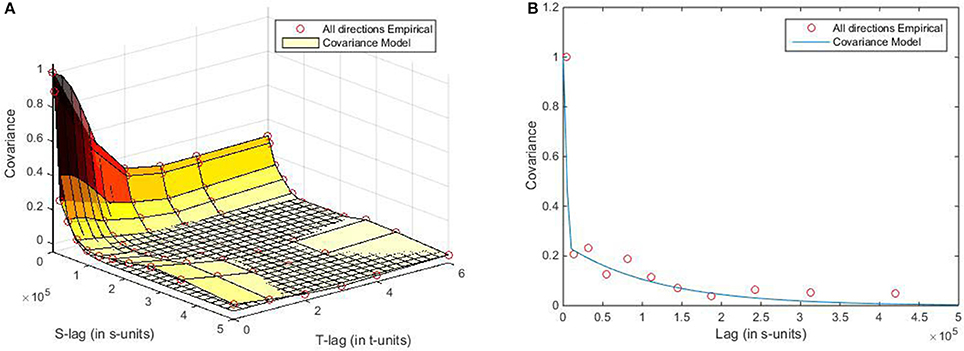
Figure 2. Plots of the spatiotemporal empirical covariances and the fitted theoretical models in (A) the R² × T domain, and (B) the R² domain.

By inserting Equation (11) into Equation (2b), the traveling coefficient was calculated to be υ = |υ| = −10650.89τ. Then, the HFRS incidence data points were projected from the R² × T domain onto the reduced dimensionality R² domain (Figure S1). Following the projection process, the empirical HFRS covariance and the fitted covariance model in the R² domain are plotted in Figure 2B, where the HFRS covariance model is analytically given by

$\begin{array}{cc}{c}_{\widehat{X}}(\widehat{h})=0.75(1-\frac{1.5\widehat{h}}{{10}^4}+\frac{0.5\widehat{h^3}}{{10}^{12}})+0.25e^{-\frac{\widehat{h}}{3.5\times {10}^5}}.& \left(12\right)\end{array}$

This covariance is also of reduced dimensionality compared to that of Equation (11). In addition, the theoretical covariance model of Equation (12) provided a better fit to the corresponding empirical covariance than the covariance model of Equation (11).

HFRS Incidence Mapping

The HFRS incidence maps were firstly generated using the P-BME technique. For illustration, the monthly HFRS incidence maps for the year 2006 (January–December) are shown in Figure 3. Additional HFRS incidence maps for all the years considered can be found in the section of “Supporting Information.”

FIGURE 3

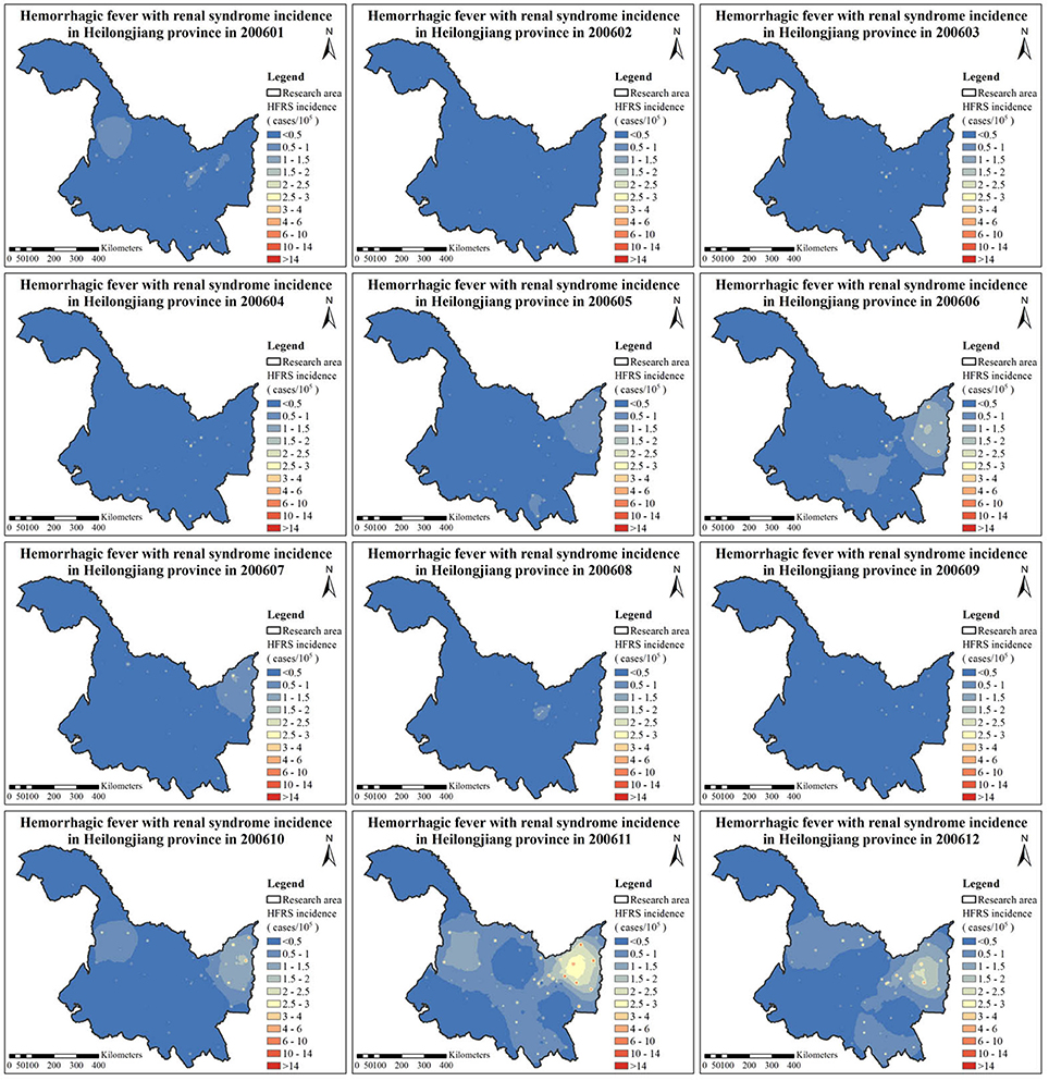
Figure 3. HFRS incidence maps during the period Jan–Dec 2006.

As regards spatial variation, three areas with considerable HFRS incidence are identified in the maps of Figure 3, particularly, in the eastern, the western and the southern parts of the Heilongjiang province. Among them, the eastern part shows high HFRS incidence values over a larger area than in the other two parts. As is noted in the section of Discussion, this happens because there exists a corresponding large area of croplands and rivers in the eastern part that are linked to increasing HFRS incidence. As regards the temporal HFRS variation in Heilongjiang province, the HFRS incidence variation exhibited two outbreaks within a year's time. Specifically, as is shown in Figure 3 and Figure S12 (Supporting Information), the HFRS incidence begins to increase in April of 2006, then a peak is reached in June of 2006, and the HFRS incidence reduces significantly in September of 2006. The next outbreak is observed during September 2006 to February 2007 with the peak occurring in November of 2006. Interestingly, the number of HFRS cases during the autumn-winter period is much larger than those during the spring-summer period. As noted in the section of Discussion, the interpretation of this phenomenon is that it is probably due to the fact that the autumn-winter period coincides with the rice harvest season, i.e., after harvest the soil condition switches from a flood state to a dry state, which leads to the rodents dispersal or migration causing a higher number of infected cases).

In the western part of the Heilongjiang province, low HFRS incidence values were observed during the months February–September of the period 2006–2013 (but not for the year 2005). The HFRS incidence at the southern part of the Heilongjiang province remained high during the months of June, October, November, and December of each year considered. Apparently, HFRS is transmitted to the southern part of the province from its eastern part. Overall, a declining trend of HFRS incidence is observed in the maps of Figures S3–S11 (Supporting Information) for the period 2005–2013, which may be due, at least in part to the development of medical condition and disease prevention.

A cross-validation analysis of P-BME mapping technique vs. direct BME mapping is plotted in Figure S2 during the years 2005–2013: specifically, the P-BME mapping was more accurate in predicting HFRS at low incidence points, whereas the direct BME mapping was more accurate in predicting HFRS incidence at high incidence points during 2005 and 2007 (see, also, the months 1–36 of the time series of HFRS incidence in Figure 4A). Overall, the P-BME was on average a better predictor of the space-time HFRS incidence distribution in the Heilongjiang province than the direct BME: the mean absolute prediction error for BME over the entire domain was 0.524 cases/100,000 individuals, whereas that of P-BME was 0.459 cases/100,000 individuals. An explanation for the above results is given in the section of Discussion below.

FIGURE 4

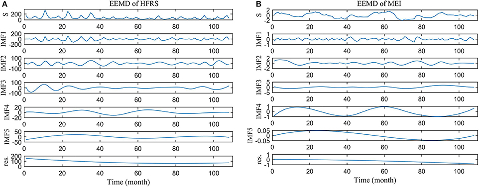
Figure 4. Ensemble EMD of (A) HFRS series and (B) MEI series. S is the original series and res. denotes the residual series.

Ensemble Empirical Mode Decomposition

Using the ensemble EMD method, five IMFs and one residual component were technically extracted from the HFRS and MEI series. The results are shown in Figure 4. In the first 40 months, the HFRS incidence series experienced much higher peaks than during the remaining months (Figure 4A), which is consistent with the findings of Figures S3–S11 (Supporting Information) above. The IMF frequency decreases from IMF1 to IMF5, whereas the corresponding IMF period increases. As it can be also seen, the long trends (residual component) of HFRS and MEI are decreasing.

Each IMF expresses a different fluctuation period (Table 1). For HFRS, the IMF1 to IMF5 represent incidence periods lasting 5.959, 8.936, 18.024, 39.002, and 64.004 months, respectively. The main HFRS inherent periods are 5.959, 8.936, and 18.024 months, according to the contribution percentage of IMF's variance. The corresponding MEI periods are 5.138, 17.662, 34.629, 50.129, and 108.466 months, respectively, whereas the main periods are 17.662, 34.629, and 50.129 months. By comparing the periods of each IMF, it was found that the IMF1 of HFRS has the same (6 months) period as the IMF1 of MEI. Similarly, the IMF3 of HFRS has the same (18 months) period with the IMF2 of MEI.

TABLE 1

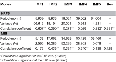
Table 1. Statistics of ensemble EMD results.

Hilbert–Huang and Marginal HFRS Incidence Spectra

The reason why the time-frequency technique (i.e., Hilbert–Huang transformation) is used at this study stage is that we seek to detect the similarities of the two series, in which case it can be concluded that the two series are inter-related. The Hilbert-Huang spectra of the HFRS and MEI series displayed in Figures 5A,B represent the time-frequency-energy distributions of the original series. As can be seen in Figures 5A,B, continuous instantaneous frequencies are detected in the low frequency region of the spectra (<0.15 cycle/month). The energy is also high in the low frequency region, especially for MEI, although some amounts of energy are detected in the middle and high frequency region of the spectra (>0.15 cycle/month).

FIGURE 5

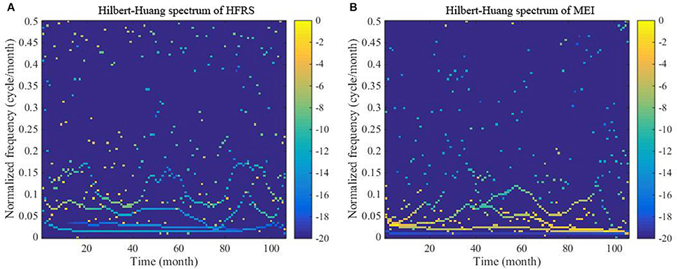
Figure 5. Hilbert-Huang spectra of (A) the HFRS series and (B) the MEI series. The color bar ranging from dark blue to yellow indicates energy variation from minimum to maximum.

Moreover, the energy associated with HFRS incidence is more discretely distributed than that associated with MEI. As is shown in Figure 6, the marginal spectra of HFRS and MEI have a similar peak occurring at ~0.015–0.025 cycle/month. Also, we notice the peaks at 0.0694 and 0.0787 cycle/month. From 0 to 0.15 cycle/month, both spectra exhibit a decreasing trend. However, the MEI spectrum decreases rapidly to a small level and the energy is concentrated in this frequency range. Compared to the marginal MEI spectrum, the marginal HFRS spectrum presents a more complex fluctuation pattern across the entire frequency domain, and the amplitude (or energy) remains above the 0.15 cycle/month threshold.

FIGURE 6

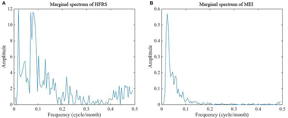
Figure 6. Marginal spectra of (A) the HFRS series and (B) the MEI series.

Wavelet Coherency Analysis

As a result of the wavelet coherency analysis we obtained the coherency wavelet spectrum between the HFRS and MEI series shown in Figure 7A. This figure indicates that there exists a strong coherency between the two series with a periodicity of 6-months band, particularly, during the sampled months 22–31, 41–52, 75–80, and 85–94. A weaker coherency was also detected around the 12-month band during the sampled months 18~28, 42~52, and 61~83.

FIGURE 7

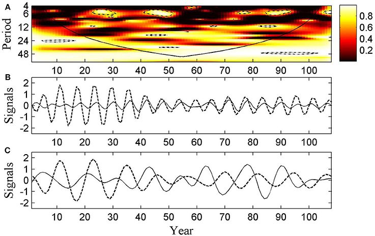
Figure 7. The HFRS-MEI association. (A) Wavelet coherency between HFRS and MEI series. The colors depict coherency values from black (0) to white (1); black line represents the cone of influence that delimits the region that is not influenced by edge effects; the dash dot line shows a = 5% significance level computed based on 500 simple bootstrap. (B) The oscillation series during the period 5–7 months band that was reconstructed from the real part of the wavelet transformed series. (C) The oscillation series during the period 8–16 months band reconstructed from the real part of the wavelet transformed series. Dash lines represent oscillation of the HFRS series, while black line represents oscillation of the MEI series.

The HFRS and MEI series reconstructed by means of the wavelet transformation are plotted in Figures 7B,C. These plots may be interpreted as providing an interesting demonstration of the HFRS and MEI series oscillations, which is useful for comparison purposes. A strong coherency is easily detected with 2 period month bands (i.e., 5–7 and 8–16 month band) during the sampled months mentioned above. This explains why the same oscillation pattern is found in Figures 7B,C.

Discussion

Public health scientists and epidemiologists are increasingly in need of gaining insight about the space-time HFRS incidence variation, and about how climate change affects HFRS incidence dynamics. This is particularly true in Heilongjiang province, which is one of the most HFRS affected areas in China. To the best of our knowledge, very few studies have used analytical methods to describe the space-time HFRS spread in Heilongjiang province. On the other hand, the associations between HFRS incidence and climate factors have been always assessed in terms of numerical modeling, for example, autoregressive integrated moving average models (ARIMA), seasonal ARIMA (SARIMA), ecological niche models (ENM), Poisson regression models, multiple regression, conditional logistic regression, and principal components regression (PCR) models [25, 34, 45–48]. Interestingly, none of these studies explored the association between HFRS incidence and climatic factors in the context of their co-variation.

Responding to the above need, the present work is a collaborative effort between the Zhejiang University (Zhoushan, China), the Institute of Disease Control and Prevention (Beijing, China), and the San Diego State University (California, USA). This collaboration led to the introduction of a combination of modern space-time modeling and mapping techniques from BME theory, Hilbert–Huang spectrum analysis and wavelet analysis in the study of the spatiotemporal HFRS incidence distribution in Heilongjiang province, and its association with climate change.

In particular, one of the main elements of this study is the implementation of the P-BME method [41] to analyze the space-time HFRS incidence spread in Heilongjiang province. Monthly HFRS incidence data were analyzed and processed across the Heilongjiang province during the period 2005–2013. Monthly HFRS data are used here because they lead to more accurate predictions than annual data (see below) and, also, they can serve better our goals to detect the temporal HFRS incidence pattern (which can be explained in ecological terms) and assess the association between the HFRS incidence pattern and climate change (MEI).

A key feature of the P-BME method is that technically it transfers the study of HFRS incidence spread from the original 3-D (i.e., two space dimensions plus time, R² × T) domain onto a reduced dimensionality 2-D (i.e., two space dimensions, R²) domain. In this way, the difficult to determine space-time distance (metric) is reduced to a much easier to define spatial distance, which means that the empirical space-time covariance of the monthly HFRS incidence distribution is accordingly transformed into a spatial covariance (see Figure 2). As a result, it is technically much easier to fit a theoretical model to the spatial than to the spatiotemporal empirical covariance of monthly HFRS data.

Next, for comparison purposes, the empirical covariances and the fitted theoretical models (in the R² × T and the R² domains) for the annual HFRS data are shown in Figure S13. This comparison shows that the temporal dependence of the annual HFRS data is much stronger than that of the monthly HFRS data (e.g., by comparing Figure 2 and Figure S13, it is seen that the annual HFRS covariance value at time lag τ = 4 is about 0.7 (cases/10⁵)² compared to 0.3 (cases/10⁵)² for the monthly covariance).

As regards the space-time mapping of HFRS spread in Heilongjiang province, it was found that the weaker the temporal dependence of the HFRS empirical covariance is, the better is the P-BME performance compared to that of the direct BME method. This improved performance of P-BME in this case is explained by the fact that since the time argument is technically imbedded within the projected coordinates of the reduced dimensionality domain, the temporal points with the stronger dependence (compared to the spatial ones) are not explicitly taken into account, instead, only traveling spatial points are considered in HFRS prediction and mapping, and the HFRS prediction error would be larger in this case. Compared to the original BME method, the P-BME was found to provide on average more accurate HFRS incidence predictions in the case of monthly HFRS incidence data (the mean absolute prediction error for P-BME is 0.459 cases/100,000 individuals vs. 0.524 cases/100,000 individuals for direct BME), whereas the opposite was the case for annual HFRS incidence data (the mean absolute prediction error for direct BME was 3.34 cases/100,000 individuals and for P-BME it was 4.56 cases/100,000 individuals).

Other findings of this study included the following. Three core areas were observed in the HFRS incidence distribution maps we obtained for the period Jan 2005–Dec 2013, particularly, the eastern, western and southern parts of Heilongjiang province. As the drainage map of Heilongjiang province shows (Figure S14), the Wusuli and Songhua rivers, as well as parts of the Heilong river belong to the eastern part, and the Neng and Mudan rivers belong to western and southern parts, respectively, of the Heilongjiang Province. Regarded as major water sources, these river basins provide a suitable environment for rodent hosts and their reproduction. The presence of a river or a pond can be a risk for human HFRS infection [49]. Bao et al. [50] found that HFRS incidence had a strong correlation with distance to rivers (in particular, HFRS incidence had a quadratic relationship with distance to rivers, and R² = 0.999, p = 0.000). On the other hand, severe droughts can significantly decrease HFRS incidence [2, 51]. As rivers can provide sufficient water for vegetation irrigation purposes, the croplands are always located near rivers, and Heilongjiang province is no exception.

In the Heilongjiang province, croplands, mixed forests, and cropland/natural vegetation mosaic account for 38.98, 26.29, and 16.92% of the territory, respectively (Figure S15). Specifically, croplands are largely distributed in the eastern and western parts of Heilongjiang province, and there are also some croplands in the southern part of Heilongjiang province, which correspond to the three core HFRS areas mentioned above. It has been found that crop production is highly correlated with HFRS incidence with a correlation coefficient r = 0.96 (p = 0.005) due to the fact that crop can directly or indirectly serve as food for rodent hosts [45]. Increasing food availability contributes to the growth of rodent host population. This can raise the infection probability of humans, especially farmers, who have a higher likelihood to come in contact with these animals [52, 53]. Farmers usually don't have steady jobs other than farming, and they also have higher mobility compared to other professions. Therefore, they may carry and spread hantaviruses to wider areas than the croplands during their traveling after the farming season. Under these conditions, HFRS may spread rapidly. Being aware of the above high HFRS spread likelihood, it is necessary to implement public health interventions in the core areas of the Heilongjiang province to avoid HFRS outbreaks and spread (these interventions include, e.g., the extermination of potential rodent hosts and vaccination).

In addition, June and November HFRS incidence peaks were found during the years 2005–2013 (Figure S12). Interestingly, this bimodal temporal pattern was also found in Hubei province after 1995, as result of the Seoul virus-related HFRS spring outbreaks and the Hantaan virus-related HFRS winter outbreaks [54]. Another study found that HFRS associated with wild and house rodents occur during different seasons [55]. In view of the fact that land-use can affect virus occurrence in hosts by influencing movement and contact rate [56, 57], we notice that Heilongjiang is located in a high latitude area, where paddy rice only grows once a year (during May and October). At the beginning of sowing season in May, soils are irrigated to remain in a flood state for paddy rice growth, and the soil conditions change from drying to flooding. After harvesting, the soil will return to drying conditions in October. These switches between different land environmental conditions may cause a cascade of factors contributing to infectious disease emergence, especially invasive alien species due to the fact that they are invaders over their natural range in the new environment [58–60]. More specifically, an agricultural ecosystem is particularly vulnerable to invasive alien species and anthropogenic activities that can initiate or accelerate the introduction or invasion of alien species [58]. Sufficient food availability during June contributes to rodent reproduction, whereas insufficient food availability or the dry conditions of November will result in spur sudden dispersal or migration events, both of which can increase HFRS infection [61]. Whats more, the edges of paddy fields may involve ecotones as habitats with infectious disease and animal reservoir hosts being abundant in wildlife [62]. Following a month-long period of environmental change, HFRS outbreaks may occur.

Generally, the study of real world phenomena is highly complex and interdisciplinary, in particular the study of large spatial scale climate and disease variation (which can be affected by biological, social, geographic, economic, medical factors etc.; [63]). Hence, the observation series may contain a large amount of direct and indirect information. With such complex information, it can be really hard for scientists to collect data from various disciplines and explore the relationship among them through hypothesis- and equation-driven methods.

In view of the above considerations, time-frequency analysis methods, regarded as data-mining tools, constitutes another major component of the present study. The results can reveal the intrinsic variation patterns of HFRS incidence and MEI series, as well as the dynamic characteristics of the HFRS and MEI cycles in the time-frequency domain. Understanding the association between HFRS incidence and climate change (using MEI as a proxy, measuring coupled oceanic-atmospheric character of ENSO event) provides a potential auxiliary way to assess the public health effects of global climate change, since climate variability has important effects on wildlife population dynamics [64, 65]. The Hilbert-Huang transformation is a powerful tool for solving mode-mixing problems and can be also used as a filter for decomposing raw HFRS incidence series into several independent series with disparate modes, i.e., IMFs [66]. Different component series were obtained that describe various inherent disease characteristics that cannot be detected in the raw series. Our results showed that both HFRS and MEI series have six types of characteristic components. A monotonic declining trend is shown in Figure 4, and both series are characterized by 6- and 18-months periods, approximately (Table 1), indicating that similar patterns are hidden in the variation features of the two series. For further analysis, the Hilbert–Huang and the marginal spectra were used to assess the strength of series variation in the combined time-frequency domain. For both series, stable and consistent variations were observed at low frequency regions, although certain discrete fluctuations can be found in the HFRS spectra that are not observed in the MEI spectra. Such differences may not be explained by climate change (MEI) but rather in terms of non-climatic factors, e.g., population immunity, public health condition, and socio-economic factors [10, 54, 67].

Moreover, wavelet coherency analysis showed that the HFRS incidence has a strong association with MEI during a 6-month period (Figure 7). These results suggest that the HFRS incidence dynamics are interrelated with climate change and the MEI can serve as a potential predictor of HFRS occurrence. We notice that similar results have been found for diseases like dengue fever, dengue hemorrhagic fever, hantavirus cardiopulmonary syndrome, and malaria [68–71]. Moreover, regional precipitation is known to be influenced by ENSO, showing the strongest interrelation with climate variability around the Globe [72]. Increasing precipitation provides sufficient soil moisture for improving ecosystem productivity [64]. As a result, the number of rodents grows rapidly, leading to increasing contact rates between rodents and between rodents and humans [61]. The HFRS infection rate increases under the above ecological changes. A deeper understanding of the association between climate change and HFRS incidence can provide a potential tool of early HFRS outbreak warning, especially concerning short-term effects.

Certain limitations of the present work should be acknowledged, which are rather typical for this kind of quantitative studies. The first one is data limitation, i.e., the HFRS dataset used is an aggregated set that does not distinguish the infectious HFRS types, e.g., Hantaan virus or Seoul virus, for which the infectious dynamics may be different. Second, the impact of climate change on human HFRS incidence can be twofold: impact from rodents to rodents and infection from rodents to humans. Therefore, distinct studies of these two possibilities would offer a better understanding of HFRS transmission. Third, some other impact factors could also be included in HFRS pattern analysis, such as population immunity and socio-economic factors. Future work should focus on a more detailed analysis of spatiotemporal intensity differences of the various environmental factors impacting HFRS incidence.

In sum, the present work provides a quantitative study of the HFRS incidence spread in Heilongjiang province (China). Three core areas with high HFRS incidences were identified. In addition, time-frequency analysis provides evidence that HFRS incidence is closely related to climate change.

Author Contributions

All authors listed have made a substantial, direct and intellectual contribution to the work, and approved it for publication.

Conflict of Interest Statement

The authors declare that the research was conducted in the absence of any commercial or financial relationships that could be construed as a potential conflict of interest.

Acknowledgments

The authors acknowledge with appreciation the Matlab codes (processing wavelet analysis) provided by Professor Bernard Cazelles. The work was supported by grants from the National Natural Science Foundation of China (No. 41671399 and No. 11501339).

Supplementary Material

The Supplementary Material for this article can be found online at: https://www.frontiersin.org/article/10.3389/fams.2017.00016/full#supplementary-material

References

1. Yan L, Fang LQ, Huang HG, Zhang LQ, Feng D, Zhao WJ, et al. Landscape elements and Hantaan virus–related hemorrhagic fever with renal syndrome, People's Republic of China. Emerg Infect Dis. (2007) 13:1301–6. doi: 10.3201/eid1309.061481

PubMed Abstract | CrossRef Full Text | Google Scholar

2. Tian H, Yu P, Bjørnstad ON, Cazelles B, Yang J, Tan H, et al. Anthropogenically driven environmental changes shift the ecological dynamics of hemorrhagic fever with renal syndrome. PLoS Pathog. (2017) 13:e1006198. doi: 10.1371/journal.ppat.1006198

PubMed Abstract | CrossRef Full Text | Google Scholar

3. Liu J, Xue FZ, Wang JZ, Liu QY. Association of haemorrhagic fever with renal syndrome and weather factors in Junan County, China: a case-crossover study. Epidemiol Infect. (2013) 141:697–705. doi: 10.1017/S0950268812001434

PubMed Abstract | CrossRef Full Text | Google Scholar

4. Chinikar S, Javadi A, Hajiannia A, Ataei B, Jalali T, Khakifirouz S, et al. First evidence of Hantavirus in central Iran as an emerging viral disease. Adv Infect Dis. (2014) 4:173–7. doi: 10.4236/aid.2014.44024

CrossRef Full Text | Google Scholar

5. Simmons JH, Riley LK. Hantaviruses: an overview. Compar Med. (2002) 52:97–110. Available online at: http://www.ingentaconnect.com/content/aalas/cm/2002/00000052/00000002/art00003

PubMed Abstract | Google Scholar

6. Krautkrämer E, Zeier M, Plyusnin A. Hantavirus infection: an emerging infectious disease causing acute renal failure. Kidney Int. (2012) 83:23–7. doi: 10.1038/ki.2012.360

PubMed Abstract | CrossRef Full Text | Google Scholar

7. Jiang H, Du H, Wang L, Wang P, Bai X. Hemorrhagic fever with renal syndrome: pathogenesis and clinical picture. Front Cell Infect Microbiol. (2016) 6:1. doi: 10.3389/fcimb.2016.00001

CrossRef Full Text | Google Scholar

8. Fang L, Yan L, Liang S, de Vlas SJ, Feng D, Han X, et al. Spatial analysis of hemorrhagic fever with renal syndrome in China. BMC Infect Dis. (2006) 6:77. doi: 10.1186/1471-2334-6-77

PubMed Abstract | CrossRef Full Text | Google Scholar

9. Zou LX, Chen MJ, Sun L. Haemorrhagic fever with renal syndrome: literature review and distribution analysis in China. Int J Infect Dis. (2016) 43:95–100. doi: 10.1016/j.ijid.2016.01.003

PubMed Abstract | CrossRef Full Text | Google Scholar

10. Zhang YZ, Zou Y, Fu ZF, Plyusnin A. Hantavirus Infections in Humans and Animals, China. Emerg Infect Dis. (2010) 16:1195–203. doi: 10.3201/eid1608.090470

PubMed Abstract | CrossRef Full Text | Google Scholar

11. Fidan K, Polat M, Isıyel E, Kalkan G, Tezer H, Söylemezoğlu O. An adolescent boy with acute kidney injury and fever: answers. Pediatr Nephrol. (2013) 28:2115–6. doi: 10.1007/s00467-012-2360-0

CrossRef Full Text | Google Scholar

12. Dearing MD, Dizney L. Ecology of hantavirus in a changing world. Ann NY Acad Sci. (2010) 1195:99–112. doi: 10.1111/j.1749-6632.2010.05452.x

PubMed Abstract | CrossRef Full Text | Google Scholar

13. Pépin M, Dupinay T, Zilber AL, McElhinney LM. Of rats and pathogens: pathogens transmitted by urban rats with an emphasis on hantaviruses. CAB Rev. (2016) 11:1–13. doi: 10.1079/PAVSNNR201611019

CrossRef Full Text

14. Li S, Ren H, Hu W, Lu L, Xu X, Zhuang D, et al. Spatiotemporal heterogeneity analysis of hemorrhagic Fever with renal syndrome in china using geographically weighted regression models. Int J Environ Res Public Health (2014) 11:12129–47. doi: 10.3390/ijerph111212129

PubMed Abstract | CrossRef Full Text | Google Scholar

15. Zhang S, Wang S, Yin W, Liang M, Li J, Zhang Q, et al. Epidemic characteristics of hemorrhagic fever with renal syndrome in China, 2006–2012. BMC Infect Dis. (2014) 14:384. doi: 10.1186/1471-2334-14-384

PubMed Abstract | CrossRef Full Text | Google Scholar

16. Zhang WY, Wang LY, Liu YX, Yin WW, Hu WB, Magalhaes RJ, et al. Spatiotemporal transmission dynamics of hemorrhagic fever with renal syndrome in China, 2005–2012. PLoS Negl Trop Dis. (2014) 8:e3344. doi: 10.1371/journal.pntd.0003344

PubMed Abstract | CrossRef Full Text | Google Scholar

17. Christakos G. A Bayesian/maximum-entropy view to the spatial estimation problem. Math Geol. (1990) 22:763–76. doi: 10.1007/BF00890661

CrossRef Full Text | Google Scholar

18. Christakos G. Spatiotemporal information systems in soil and environmental sciences. Geoderma (1998) 85:141–79. doi: 10.1016/S0016-7061(98)00018-4

CrossRef Full Text | Google Scholar

19. Christakos G. Modern Spatiotemporal Geostatistics. New York, NY: Oxford University Press (2000).

Google Scholar

20. He, J, Kolovos, A. Bayesian maximum entropy approach and its applications: a review. Stoch Environ Res Risk Assess. (2017) doi: 10.1007/s00477-017-1419-7. [Epub ahead of print].

CrossRef Full Text | Google Scholar

21. Law DCG, Bernstein KT, Serre ML, Schumacher CM, Leone PA, Rompalo AM, et al. Modeling a syphilis outbreak through space and time using the Bayesian maximum entropy approach. Ann Epidemiol. (2006) 16:797–804. doi: 10.1016/j.annepidem.2006.05.003

CrossRef Full Text | Google Scholar

22. Choi KM, Yu HL, Wilson ML. Spatiotemporal statistical analysis of influenza mortality risk in the State of California during the period 1997–2001. Stoch Environ Res Risk Assess. (2008) 22:15–25. doi: 10.1007/s00477-007-0168-4

CrossRef Full Text | Google Scholar

23. Clement J, Vercauteren J, Verstraeten WW, Ducoffre G, Barrios JM, Van Ranst A-M, et al. Relating increasing hantavirus incidences to the changing climate: the mast connection. Int J Health Geogr. (2009) 8:1. doi: 10.1186/1476-072X-8-1

PubMed Abstract | CrossRef Full Text | Google Scholar

24. Zhang WY, Guo WD, Fang LQ, Li CP, Bi P, Glass GE, et al. Climate variability and hemorrhagic fever with renal syndrome transmission in Northeastern China. Environ Health Perspect. (2010) 118:915–20. doi: 10.1289/ehp.0901504

PubMed Abstract | CrossRef Full Text | Google Scholar

25. Liu X, Jiang B, Gu W, Liu Q. Temporal trend and climate factors of hemorrhagic fever with renal syndrome epidemic in Shenyang City, China. BMC Infect Dis. (2011) 11:331. doi: 10.1186/1471-2334-11-331

PubMed Abstract | CrossRef Full Text | Google Scholar

26. Xiao H, Tian HY, Cazelles B, Li XJ, Tong SL, Gao LD, et al. Atmospheric moisture variability and transmission of hemorrhagic fever with renal syndrome in Changsha City, Mainland China, 1991–2010. PLoS Negl Trop Dis. (2013) 7:e2260. doi: 10.1371/journal.pntd.0002260

PubMed Abstract | CrossRef Full Text | Google Scholar

27. Tian HY, Yu PB, Luis AD, Bi P, Cazelles B, Laine M, et al. Changes in rodent abundance and weather conditions potentially drive hemorrhagic fever with renal syndrome outbreaks in Xi'an, China, 2005–2012. PLoS Negl Trop Dis. (2015) 9:e0003530. doi: 10.1371/journal.pntd.0003530

PubMed Abstract | CrossRef Full Text | Google Scholar

28. Huang NE, Shen Z, Long SR, Wu MC, Shih HH, Zheng Q, et al. The empirical mode decomposition and the Hilbert spectrum for nonlinear and non-stationary time series analysis. Proc R Soc A (1998) 454:903–95. doi: 10.1098/rspa.1998.0193

CrossRef Full Text | Google Scholar

29. Huang NE, Wu ML, Qu W, Long SR, Shen SS. Applications of Hilbert–Huang transform to non-stationary financial time series analysis. Appl Stoch Models Bus Indus. (2003) 19:245–68. doi: 10.1002/asmb.501

CrossRef Full Text | Google Scholar

30. Huang NE, Wu Z. A review on Hilbert-Huang transform: method and its applications to geophysical studies. Rev Geophys. (2008) 46:RG2006. doi: 10.1029/2007RG000228

CrossRef Full Text | Google Scholar

31. Grinsted A, Moore JC, Jevrejeva S. Application of the cross wavelet transform and wavelet coherence to geophysical time series. Nonlin Process Geophys. (2004) 11:561–6. doi: 10.5194/npg-11-561-2004

CrossRef Full Text | Google Scholar

32. Thai KT, Cazelles B, Van Nguyen N, Vo LT, Boni MF, Farrar J, et al. Dengue dynamics in Binh Thuan province, southern Vietnam: periodicity, synchronicity and climate variability. PLoS Negl Trop Dis. (2010) 4:e747. doi: 10.1371/journal.pntd.0000747

PubMed Abstract | CrossRef Full Text | Google Scholar

33. Chowell G, Cazelles B, Broutin H, Munayco CV. The influence of geographic and climate factors on the timing of dengue epidemics in Perú, 1994-2008. BMC Infect Dis. (2011) 11:164. doi: 10.1186/1471-2334-11-164

PubMed Abstract | CrossRef Full Text | Google Scholar

34. Li CP, Cui Z, Li SL, Magalhaes RJS, Wang BL, Zhang C, et al. Association between hemorrhagic fever with renal syndrome epidemic and climate factors in Heilongjiang Province, China. Am J Trop Med Hyg. (2013) 89:1006–12. doi: 10.4269/ajtmh.12-0473

PubMed Abstract | CrossRef Full Text | Google Scholar

35. Curran LM, Caniago I, Paoli GD, Astianti D, Kusneti, M, Haeruman H. Impact of El niño and logging on canopy tree recruitment in borneo. Science (1999) 286:2184–8. doi: 10.1126/science.286.5447.2184

PubMed Abstract | CrossRef Full Text | Google Scholar

36. Wolter K, Timlin MS. El Niño/Southern oscillation behaviour since 1871 as diagnosed in an extended multivariate ENSO index (MEI. ext). Int J Climatol. (2011) 31:1074–87. doi: 10.1002/joc.2336

CrossRef Full Text | Google Scholar

37. Christakos G. Spatiotemporal Random Fields: Theory and Applications. Amsterdam: Elsevier (2017).

38. Reyes JM, Serre ML. An LUR/BME framework to estimate PM2. 5 explained by on road mobile and stationary sources. Environ Sci Technol. (2014) 48:1736–44. doi: 10.1021/es4040528

PubMed Abstract | CrossRef Full Text | Google Scholar

39. Kyriakidis PC, Journel AG. Geostatistical space–time models: a review. Math Geol. (1999) 31:651–84. doi: 10.1023/A:1007528426688

CrossRef Full Text | Google Scholar

40. Stein ML. Space–time covariance functions. J Am Stat Assoc. (2005) 100:310–21. doi: 10.1198/016214504000000854

CrossRef Full Text | Google Scholar

41. Christakos G, Zhang C, He J. A traveling epidemic model of space–time disease spread. Stoch Environ Res Risk Assess. (2017) 31:305–14. doi: 10.1007/s00477-016-1298-3

CrossRef Full Text | Google Scholar

42. Wu Z, Huang N. Ensemble empirical mode decomposition: a noise-assisted data analysis method. Adv Adapt Date Anal. (2009) 01:1–41. doi: 10.1142/S1793536909000047

CrossRef Full Text | Google Scholar

43. Ju K, Zhou D, Zhou P, Wu J. Macroeconomic effects of oil price shocks in China: an empirical study based on Hilbert–Huang transform and event study. Appl Energy (2014) 136:1053–66. doi: 10.1016/j.apenergy.2014.08.037

CrossRef Full Text | Google Scholar

44. Cazelles B, Chavez M, Berteaux D, Ménard F, Vik JO, Stenseth NC, et al. Wavelet analysis of ecological time series. Oecologia (2008) 156:287–304. doi: 10.1007/s00442-008-0993-2

PubMed Abstract | CrossRef Full Text | Google Scholar

45. Bi P, Wu X, Zhang F, Parton KA, Tong S. Seasonal rainfall variability, the incidence of hemorrhagic fever with renal syndrome, and prediction of the disease in low-lying areas of China. Am J Epidemiol. (1998) 148:276–81. doi: 10.1093/oxfordjournals.aje.a009636

PubMed Abstract | CrossRef Full Text | Google Scholar

46. Xiao H, Gao L, Li X, Lin X, Dai X, Zhu P, et al. Environmental variability and the transmission of haemorrhagic fever with renal syndrome in Changsha, People's Republic of China. Epidemiol Infect. (2013) 141:1867–75. doi: 10.1017/S0950268812002555

PubMed Abstract | CrossRef Full Text | Google Scholar

47. Xiao H, Lin X, Gao L, Huang C, Tian H, Li N, et al. Ecology and geography of hemorrhagic fever with renal syndrome in Changsha, China. BMC Infect Dis. (2013) 13:305. doi: 10.1186/1471-2334-13-305

PubMed Abstract | CrossRef Full Text | Google Scholar

48. Xiao H, Liu HN, Gao LD, Huang CR, Li Z, Lin XL, et al. Investigating the effects of food available and climatic variables on the animal host density of hemorrhagic fever with renal syndrome in Changsha, China. PLoS ONE (2013) 8:e61536. doi: 10.1371/journal.pone.0061536

PubMed Abstract | CrossRef Full Text | Google Scholar

49. Li J, Chen Z, Hou T, Xing Y, Cai Z, Yang Y. Study on the risk factors of hemorrhagic fever with renal syndrome in Xi'an City (in Chinese). Chin J Dis Control Prevent. (2013) 17:564–6. Available online at: http://www.cqvip.com/qk/80677a/201307/46406708.html

50. Bao C, Liu W, Zhu Y, Liu W, Hu J, Liang Q, et al. The spatial analysis on hemorrhagic fever with renal syndrome in Jiangsu Province, China based on geographic information system. PLoS ONE (2014) 9:e83848. doi: 10.1371/journal.pone.0083848

PubMed Abstract | CrossRef Full Text | Google Scholar

51. Yang H, Xia X, Wu Y. Analysis of trend and impact factors of hemorrhagic fever with renal syndrome in Xi'an City, 1999-2000 (in Chinese). In: First Annual Academic Conference of Chinese Preventive Medicine Association (Jinan) (2002), p. 330–1. Available online at: http://cpfd.cnki.com.cn/Article/CPFDTOTAL-ZHYF200208001678.htm

52. Ruo SL, Li YL, Tong Z, Ma QR, Liu ZL, Fisher-Hoch SP. Retrospective and prospective studies of hemorrhagic fever with renal syndrome in rural China. J Infect Dis. (1994) 170:527–34. doi: 10.1093/infdis/170.3.527

PubMed Abstract | CrossRef Full Text | Google Scholar

53. Engelthaler DM, Mosley DG, Cheek JE, Levy CE, Komatsu KK, Frampton JW. Climatic and environmental patterns associated with hantavirus pulmonary syndrome, Four Corners region, United States. Emerg Infect Dis. (1999) 5:87. doi: 10.3201/eid0501.990110

PubMed Abstract | CrossRef Full Text | Google Scholar

54. Zhang YH, Ge L, Liu L, Huo XX, Xiong HR, Liu YY, et al. The epidemic characteristics and changing trend of hemorrhagic fever with renal syndrome in Hubei Province, China. PLoS ONE (2014) 9:e92700. doi: 10.1371/journal.pone.0092700

PubMed Abstract | CrossRef Full Text | Google Scholar

55. Chen HX, Qiu FX, Dong BJ, Ji SZ, Li YT, Wang Y, et al. Epidemiological studies on hemorrhagic fever with renal syndrome in China. J Infect Dis. (1986) 154:394–8. doi: 10.1093/infdis/154.3.394

PubMed Abstract | CrossRef Full Text | Google Scholar

56. Klempa B. Hantaviruses and climate change. Clin Microbiol Infect. (2009) 15:518–23. doi: 10.1111/j.1469-0691.2009.02848.x

PubMed Abstract | CrossRef Full Text | Google Scholar

57. Zhang W-Y, Fang L-Q, Jiang J-F, Hui F-M, Glass GE, Yan L, et al. Predicting the risk of hantavirus infection in Beijing, People's Republic of China. Am J Trop Med Hyg. (2009) 80:678–83. doi: 10.4269/ajtmh.2009.80.678

PubMed Abstract | CrossRef Full Text | Google Scholar

58. McNeely JA, Mooney HA, Neville LE, Schei PJ, Waage J (eds.). Global Strategy on Invasive Alien Species. Gland: IUCN (2001).

Google Scholar

59. Patz JA, Daszak P, Tabor GM, Aguirre AA, Pearl M, Epstein J, et al. Unhealthy landscapes: policy recommendations on land use change and infectious disease emergence. Environ Health Perspect. (2004) 112:1092–8. doi: 10.1289/ehp.6877

PubMed Abstract | CrossRef Full Text | Google Scholar

60. Tian H, Huang S, Zhou S, Bi P, Yang Z, Li X, et al. Surface water areas significantly impacted 2014 dengue outbreaks in Guangzhou, China. Environ Res. (2016) 150:299–305. doi: 10.1016/j.envres.2016.05.039

PubMed Abstract | CrossRef Full Text | Google Scholar

61. Parmenter RR, Yadav EP, Parmenter CA, Ettestad P, Gage KL. Incidence of plague associated with increased winter-spring precipitation in New Mexico. Am J Trop Med Hyg. (1999) 61:814–21. doi: 10.4269/ajtmh.1999.61.814

PubMed Abstract | CrossRef Full Text | Google Scholar

62. Despommier D, Ellis BR, Wilcox BA. The role of ecotones in emerging infectious diseases. Ecohealth (2006) 3:281–9. doi: 10.1007/s10393-006-0063-3

CrossRef Full Text | Google Scholar

63. Moustakas A. Spatio-temporal data mining in ecological and veterinary epidemiology. Stoch Environ Res Risk Assess. (2017) 31:829–34. doi: 10.1007/s00477-016-1374-8

CrossRef Full Text | Google Scholar

64. Stenseth NC, Mysterud A, Ottersen G, Hurrell JW, Chan KS, Lima M. Ecological effects of climate fluctuations. Science (2002) 297:1292–6. doi: 10.1126/science.1071281

PubMed Abstract | CrossRef Full Text | Google Scholar

65. Patz JA, Campbell-Lendrum D, Holloway T, Foley JA. Impact of regional climate change on human health. Nature (2005) 438:310–7. doi: 10.1038/nature04188

PubMed Abstract | CrossRef Full Text | Google Scholar

66. Tsai FF, Fan SZ, Lin YS, Huang NE, Yeh JR. Investigating power density and the degree of nonlinearity in intrinsic components of anesthesia EEG by the hilbert-huang transform: an example using ketamine and alfentanil. PLoS ONE (2016) 11:e0168108. doi: 10.1371/journal.pone.0168108

PubMed Abstract | CrossRef Full Text | Google Scholar

67. Song G. Epidemiological progresses of hemorrhagic fever with renal syndrome in China. Chin Med J. (1999) 112:472–7.

PubMed Abstract | Google Scholar

68. Hay SI, Myers MF, Burke DS, Vaughn DW, Endy T, Rogers DJ. Etiology of interepidemic periods of mosquito-borne disease. Proc Natl Acad Sci USA. (2000) 97:9335–9. doi: 10.1073/pnas.97.16.9335

PubMed Abstract | CrossRef Full Text | Google Scholar

69. Hjelle B, Glass GE. Outbreak of hantavirus infection in the four corners region of the United States in the wake of the 1997–1998 El Nino—Southern oscillation. J Infect Dis. (2000) 181:1569–73. doi: 10.1086/315467

PubMed Abstract | CrossRef Full Text | Google Scholar

70. Zhou G, Minakawa N, Githeko AK, Yan G. Association between climate variability and malaria epidemics in the East African highlands. Proc Natl Acad Sci USA. (2004) 101:2375–80. doi: 10.1073/pnas.0308714100

PubMed Abstract | CrossRef Full Text | Google Scholar

71. Tipayamongkholgul M, Fang CT, Klinchan S, Liu CM, King CC. Effects of the El Niño-Southern Oscillation on dengue epidemics in Thailand, 1996-2005. BMC Public Health (2009) 9:422. doi: 10.1186/1471-2458-9-422

PubMed Abstract | CrossRef Full Text | Google Scholar

72. Ropelewski CF, Halpert MS. Global and regional scale precipitation patterns associated with the El Niño/Southern Oscillation. Monthly Weather Rev. (1987) 115:1606–26.

Google Scholar