Applicability of the Analytical Solution to N-Person Social Dilemma Games

1. Introduction

Agent based social simulation is a common method to analyze N-person social dilemma games. The research on this topic started in the 1990s [1, 2] and has been used to study artificial societies, world politics, law, and other fields [3, 4–6]. In this paper the applicability of the analytical solution of such games with Pavlovian agents in a two dimensional cellular automaton environment is explored when the agents' decision to cooperate or defect is based on reinforcement learning with linear payoff functions. The specific model used in this paper has earlier been used to study prisoner's dilemma cooperation in a socio-geographic community [7] and a chicken dilemma selection between public transport and a car in a large city [8]. The applicability of the analytic solution depends on the way of considering the fact that all probability values have to be between 0 an 1, which was not taken into account in these earlier works. N-person social dilemma games and this model can also be used to analyze such areas as military expenditures, oil cartels, and climate change. The model examined in this paper is equivalent to the one used in Merlone et al. [9] to develop an analytical model for the N-Person prisoners' dilemma game. A new systematic review of the n-person social dilemma game is given in Merlone et al. [10] based on the dynamic properties the corresponding systems. This paper is intended to follow-up on the research presented in the above mentioned papers. The following paragraphs give an overview of this model.

Two player social dilemma games are described with a symmetric matrix based on parameters P, R, S, and T. In this matrix R is the payoff for both agents if they cooperate, P is the payoff for both agents if they defect, S is the payoff for a cooperating agent if the other agent defects, and T is the payoff for a defecting agent if the other agent cooperates. These parameters are real numbers and derived from the Prisoners' Dilemma game and are referred to as Punishment (P), Reward (R), Sucker's Bet (S), and Temptation (T). Social games are defined by the relationship between the parameters P, R, S, and T. The signs of these parameter values are not specified, only their orders of magnitude count. For example, Prisoner's Dilemma occurs when the parameters of the payoff functions satisfy the relation T > R > P > S. There are 24 different potential games since there are 4! = 24 different orderings of these four parameters. Discussion, classification, and stability of these symmetric and unsymmetric two player games can be found in Rapoport and Guyer [11]. In this paper we will assume R > P. We can do this without loss of generality since if R < P for a particular game then we simply interchange the definitions of cooperation and defection to derive an equivalent game with R > P. This means there are 12 unique games, each having its own conditions and story. These games include Prisoners' Dilemma, Chicken, Leader, Battle of the Sexes, Stag Hunt, Harmony, Coordination, and Deadlock. In addition, for most of this paper we will assume that reward R is a positive payoff and that punishment P is a negative payoff. Later in this paper, the special cases were R and P are either both positive or both negative will be investigated.

In multi-person or N-person social games the model takes into account the collective behavior in society where individual agents may cooperate with each other for the collective best interests or defect to pursue their own self interest. This paper assumes that Pavlovian agents are interacting with each other in a two dimensional cellular automaton environment. The Pavlovian agent is defined in Szilagyi [12] and studied in Merlone et al. [9] among others, as an agent having certain probability p of cooperating in each time period based on Thorndike's law of conditioning [13]; actually in Merlone et al. [9] they are called Skinnerian. The algorithm computing these probabilities will be presented in section 2 and is based on reinforcement learning. In general terms the probability to cooperate increases if either the cooperating agent is rewarded or defecting agent is punished; and the probability to cooperate decreases if either the cooperating agent is punished or defecting agent is rewarded. Similar reinforcement algorithms and models primarily used for repeated games can be found in the literature [14–16].

This paper will assume linear payoff functions as shown in the left hand side of Figure 1. Variable x is the percentage of cooperators, C(x) is the payoff for those agents that are cooperating and D(x) is the payoff for those agents that are defecting. The right hand side of Figure 1 shows the simulation results with these payoff functions performed on a 50 × 50 cellular automaton grid with each Pavlovian agent having an initial cooperating probability 0.5 and equal learning factors 0.05. The figure shows the percentage of cooperators in the automaton grid after each iteration. The results show that the percentage of cooperators reaches a steady state around 0.2 after about 50 iterations.

FIGURE 1

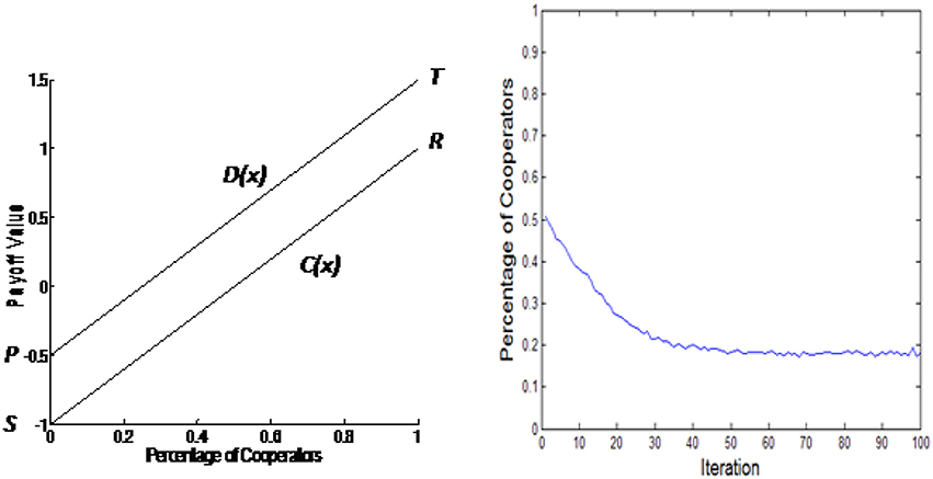
Figure 1. Linear payoff functions and simulation results.

The model moves forward in the iteration process. In each iteration agents simultaneously decide to cooperate or defect based on their probability p to cooperate. In the first iteration this is an assigned initial condition and in subsequent iterations it is determined by the reinforcement learning algorithm. As previously stated this algorithm will be presented in section 2. It is based on the payoff functions, learning factors, neighborhood size, the percentage of cooperators in the system, and whether the agent cooperates or defects. The percentage of cooperators of the entire grid is determined and used as a statistic to evaluate the state of the system. This repeats for the designated number of iterations.

A three dimensional simulation plot with varying payoff function parameters is shown in Figure 2. In this figure each mesh intersection represents the percentage of cooperators at the end of a simulation run on a 50 × 50 cellular automaton grid with each Pavlovian agent having an initial cooperating probability 0.5 and equal learning factors 0.05. For this simulation each T and S axis is broken into 40 subdivisions. Thus, Figure 2 represents the results of 1,600 single simulation runs, each with different values of T and S. There are three plateaus with varying agent behavior in each plateau. In the Prisoners' Dilemma plateau each agent's cooperating probability fluctuates around a steady state equilibrium. These agents are called bipartisan since they are willing to change their minds from iteration to iteration. In the Leader and Battle of the Sexes games each agent decides to either cooperate or defect and then never change their minds. These agents are called partisan because of their reluctance to change decision. In the Harmony/Deadlock plateau all agents decide to cooperate. These agents are called unison since they all make the same decision.

FIGURE 2

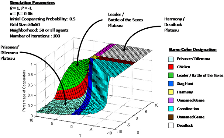
Figure 2. Simulation result with varying S and T values.

This paper is intended to be a follow-up to the works of Szilagyi [12] and Merlone et al. [9]. In these papers analytical solutions are presented with verification using agent based simulation for some specific Prisoner's Dilemma examples, however no exhaustive analysis is given on the conditions where it is applicable. In Merlone et al. [10] the dynamic properties of the corresponding system are the main focus without examining the applicability of the analytical solution. The purpose of this paper is to evaluate where the analytical solution works using the foundations from the previous works. In section 2.1 the analytical solution is derived and plotted on a S vs. T graph similarly to Figure 2. The simulation result and analytical solution are compared over the S vs. T range for a specific case of the R and P values. It is found that the simulation results and analytical solution are within 0.01 of each other in certain portions of the Prisoner's Dilemma, Chicken, Leader, Stag Hunt, and Coordination games. Section 2.2 analyzes the boundaries where the analytical solution is working. In this section some arbitrary judgments and comparisons are made in order to determine these boundaries. In section 2.3 a special approach is used to assess where the analytical solution is working without the use of these arbitrary judgments and comparisons. In section 3 the results are reviewed by varying initial cooperating probability, neighborhood size, learning factors and the values of S. Finally, section 4 summarizes the main results and presents conclusions.

2. Analysis

2.1. Analytic Solution

In this section we will develop the analytical solution to the social dilemma game. The review of this analysis is a key component in determining where the analytical solution coincides with simulation results. First the expected value of an agent's cooperating probability in the next time period will be determined given the agent's current cooperating probability and percentage of cooperators in the system at the current time. From that the expected percentage of cooperators in the next time period is developed given the current percentage of cooperators. The steady state percentage of cooperators is then given by the value where the percentage of cooperators does not change from the current to the next time period. In this paper linear payoff functions are assumed, however up to this point the analysis is valid for general payoff functions. So, finally the analytical solution for the steady state percentage of cooperators will be given for linear payoff functions in terms of model parameters α, β, P, R, S, and T. This interaction of the agents is the basis of the agent based analysis and simulation.

The probability that an agent i will be cooperating in the next period can be represented by

$\begin{array}{ll}{p}_i^{\text{new}}=\{\begin{array}{ll}{p}_i+\alpha C\left(x\right)\hfill & \text{if the agent is a cooperator}\hfill \\ p_i-\beta D\left(x\right)\hfill & \text{if the agent is a defector}\hfill \end{array}& (1)\end{array}$

where x is the current percentage of cooperators, α and β are real valued learning factors and $p_i^{\mathrm{\text{new}}}$ denotes the probability that an agent i will be cooperating in the next time period and x the percentage of the cooperating agents during the current time period. C(x) is the payoff for cooperating agents and D(x) is the payoff for the defecting agents. The behavior of each agent in the next time period depends on the current behavior of all agents through the percentage of cooperators. This interaction is the basis of the agent based analysis and simulation. The agents also learn about their cooperating probabilities through Equation (1). Since $p_i^{\mathrm{\text{new}}}$ is a percentage, it has to be between 0 and 1, which is not guaranteed by Equation (1). If its value becomes negative, then it is adjusted to zero and if it becomes larger than 1, then its value is adjusted to 1. A key assumption in the following derivation is that the new cooperating probability is obtained without the use of these adjustments. That is, this derivation will not be applicable in scenarios where the cooperating probability for an agent either is consistently going negative and be adjusted to zero or going above one and being adjusted to one. These adjustments are not accounted for in the derivation, since it would become complicated by accounting for the probabilities P(p_i < 0) and P(p_i > 1) which are not known.

First we obtain the expected value of an agent's cooperating probability in the next time period. By definition an agent is a cooperator with probability p_i and a defector with probability 1−p_i. Given these probabilities the expected value of $p_i^{\mathrm{\text{new}}}$ becomes

$\begin{array}{l}\text{E}(p_i^{\text{new}})=\left[p_i+\alpha C(x)\right]p_i+\left[p_i-\beta D(x)\right](1-p_i)\\ =\left[\alpha C(x)+\beta D(x)+1\right]p_i-\beta D(x)& (2)\end{array}$

Now the percentage of cooperating agents will be evaluated and the steady state determined. If N is the total number of agents, then the percentage of the cooperating agents is $x=\frac{1}{N}{\sum }_{i=1}^N{p}_i$. By combining this relation and Equation (2) we have

$\begin{array}{ll}{x}^{\mathrm{\text{new}}}=\frac{1}{N}{\displaystyle \sum _{i=1}^N}\mathrm{\text{E}}(p_i^{\mathrm{\text{new}}})=\left[\alpha C(x)+\beta D(x)+1\right]x-\beta D(x).& (3)\end{array}$

At any steady state x, x^new does not change from x. That is, if x = x*, then x^new = x* as well. Therefore, from Equation (3) we conclude that x* is a steady state if and only if

$x^{*}=\left[\alpha C(x^{*})+\beta D(x^{*})+1\right]x^{*}-\beta D(x^{*}),$

which can be written as

$\begin{array}{ll}{x}^{*}\alpha C(x^{*})=(1-x^{*})\beta D(x^{*}).& (4)\end{array}$

The above analysis is valid in the case of general payoff functions since in the above derivation no special forms are assumed. In the linear case C(x) = S + (R − S)x and D(x) = P + (T − P)x, so Equation (4) becomes

$\begin{array}{ll}{x}^{*}\alpha \left[S+(R-S)x^{*}\right]=(1-x^{*})\beta \left[P+(T-P)x^{*}\right].& (5)\end{array}$

This is a quadratic equation for x* and therefore there are at most two steady states. The solutions of Equation (5) are as follows:

$\begin{array}{ll}{x}^{*}=\frac{-\alpha S-2\beta P+\beta T\pm \sqrt{{\alpha }^2{S}^2-2\alpha \beta ST+{\beta }^2{T}^2+4\alpha \beta PR}}{2(\alpha R-\alpha S+\beta T-\beta P)}.& (6)\end{array}$

Figure 3 shows the analytical solutions using parameters R = 1 and P = −1 , with T and S varying between −10 and 10 with learning factors α = β = 0.05. These values of the learning factors will be used later in all simulation cases except in Figure 12, where the learning factors will be lowered and the dependence on the values of the learning factors will be examined. The left hand graph in the figure represents the lower or smaller real root and the right hand side represents the larger real root. Since there is no quantitative restriction on Equation (6) the roots or solutions may not be real, or they could be real but may be negative or greater than one. In these graphs whenever the solution is negative, the percentage of cooperators is adjusted to zero and if the solution is greater than one than the percentage of cooperators is adjusted to one. This occurs in the region with high positive S and high negative T. Specifically in this case it occurs when S−T > 2. Obviously in this region the analytical solution is not going to work since it is giving percentages of cooperators below zero and above one. Also, it is expected that the analytical solution will not be applicable if the analytical solution is giving complex roots. This occurs when $|\beta T-\alpha S|\ge 2\sqrt{-\alpha \beta PR}$ or in this specific case |T − S| < 2. This can be seen in both charts as a flat strip with a value of 0.5 running in the region where |T − S| < 2. Thus, the only region where the analytical solution may work is when |T − S| > 2. By comparing the two solutions to Figure 2 it appears by observation that the smaller analytical solution in the left hand side may approximate the simulation in Figure 2 in the Prisoners' Dilemma Plateau.

FIGURE 3

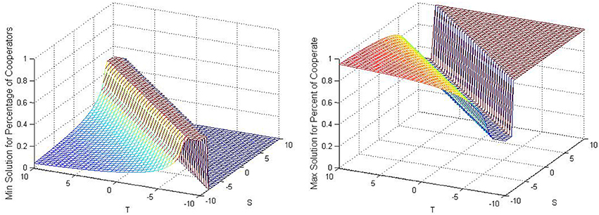
Figure 3. Analytical solutions with R = 1 and P = −1.

Figure 4 presents the same simulation results as in Figure 2 with the addition of a black region which compares the simulation results to the analytical solution. In addition to presenting the simulation results with the Figure 2 parameter values, the solution x* in Equation (6) for each point is determined and compared against the simulation result. A black region has been added to this plot whenever the simulation result and x* are within 0.01. Thus, the black region shows where the analytical solutions are close to the simulation results. This tolerance of 0.01 was assigned arbitrarily in order to determine when the analytical solution starts detracting from the simulation results. The plot on the right side is a top down view of the isometric view shown on the left hand side. The top down view with black regions to depict where the simulation results and analytical solution are within 0.01 is used often in this paper. These figures indicate that the analytical solution is within 0.01 of the simulation results in portions of Prisoner's Dilemma, Chicken, Leader, Stag Hunt, and Coordination games.

FIGURE 4

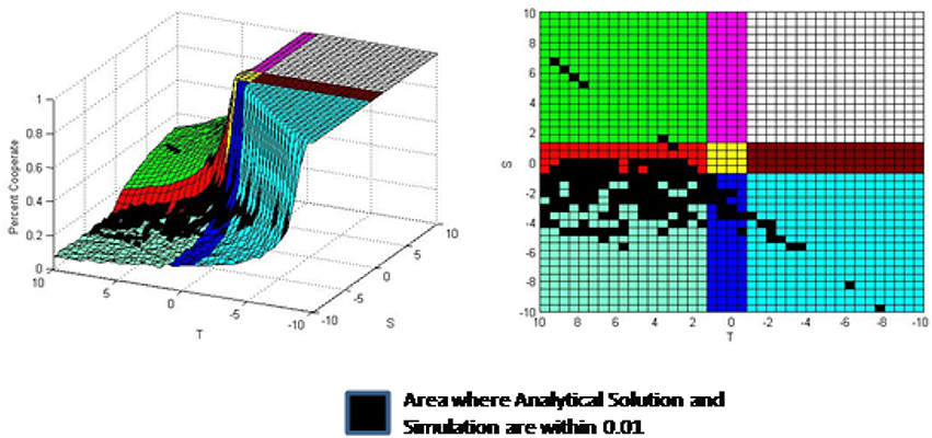
Figure 4. Comparison between simulation results and analytical solution.

2.2. Analysis of Boundaries Around Analytical Solution

From the comparison results shown in Figure 4 three boundaries can be observed around regions where the analytical solution is close to the simulation results. Figure 5 repeats Figure 4 with these boundaries. The black singular dots outside of the boundaries are not areas where the analytical solution is working. These isolated dots are where plane of Figure 2 obtained by simulation intercepts the analytical solution plane of Figure 3 after diverging from the boundary area. The first boundary which will be discussed in this section is the line T − S = 2 where the transition between the Prisoner's Dilemma and Harmony/Deadlock transition occurs. This is shown as a gray line in Figure 5. The second boundary is the transition between the Prisoners' Dilemma and Leader/Battle of the Sexes Plateaus occurring at S = 0. This is shown as a white line. Finally, the third boundary is occurring at the points with higher negative S values within the Prisoners' Dilemma game. This boundary is shown as a dashed line. This third boundary is less distinct than the first two and is arbitrarily inserted where it appears the black region starts to disappear.

FIGURE 5

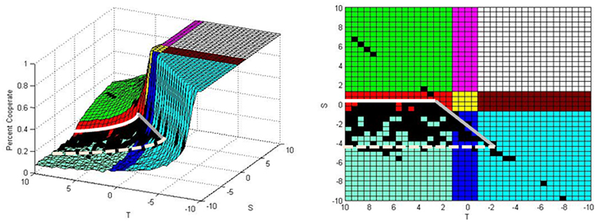
Figure 5. Analytical solution boundaries.

The fact that the derivation of the analytical solution does not account for any adjustment of probabilities comes up in evaluating all the boundaries. That is, the analytical solution is not expected to work in the Leader and Battle of the Sexes games because in this plateau the agents either cooperate with certainty or defect with certainty. The cooperating probabilities of the agents are either going negative and being adjusted to zero or raising greater than one and being adjusted to unity. It is also true that the analytical solution is not expected to work in the Harmony/Deadlock Plateau since all agents have unison behavior by cooperating with certainty with their cooperating probabilities raising above one and being adjusted to unity 100% of the time.

First we will look at the transition between the Prisoners' Dilemma and Harmony/Deadlock Plateaus. This is a steep transition where the agent behavior changes from bipartisan to unison. As stated above, it is expected that the analytical solution will not work in the Harmony/Deadlock plateau as the agents have unison behavior. That is, the cooperating probability for each agent in this plateau is greater than one and being adjusted to one. By observation of Figure 5 it appears that the boundary is, in fact, the transition when the roots to the analytical solution become complex which is the line $\beta T-\alpha S=2\sqrt{-\alpha \beta PR}$ previously derived. This boundary was confirmed also by using other reward (R = 1, 3, 5) and punishment (P = −1, −3, −5) parameter values.

Now we will look at the transition between the Prisoners' Dilemma Plateau and the Leader/Battle of the Sexes plateau. This transition is a step increase where the agent behavior changes from bipartisan to partisan. Moving from the Prisoners' Dilemma Plateau to the Leader/Battle of the Sexes Plateau the bipartisan behavior disappears when S goes from negative to positive. Therefore, the analytical solution will not work when S > 0 because there is no bipartisan behavior. Thus, S < 0 is needed for the analytical solution to work. This boundary was also confirmed by using other reward (R = 1, 3, 5) and punishment (P = −1, −3, −5) parameter values.

The last region to be explored is within the Prisoner's Dilemma Plateau when S becomes more negative. The simulation results diverging from the analytical solution in this region is not as obvious or distinct as in the previous two cases because in this region the agents are acting in a bipartisan manner with their cooperating probabilities fluctuating around a steady state as it was assumed in the derivation of the analytical solution. The problem is that as S becomes more negative, the agents become more severely punished per Equation (1) when they cooperate. At some point the punishment becomes so large that some agents' cooperating probabilities become negative if they cooperate during multiple consecutive iterations and then their cooperating probabilities have to be adjusted to zero. Then the agents cooperating probabilities rise above zero upon a defection on the next iteration and then may fluctuate around the steady state until the next severe punishment occurs for multiple consecutive cooperating decisions. If the value of S is only marginally high negative, then the punishment will result in only slight adjustments and the analytical solution will be close to the simulation results. As S becomes more negative, the punishment becomes higher for cooperation so greater adjustments are required to bring the cooperating probability to zero, which implies that the analytical solution will not be a close estimate. As an example, Figure 6 shows a simulation run on a 20 × 20 grid with R = 1, P = −1, T = 1, and S = −9. The figure shows the cooperating probabilities for each agent during the final iteration. It can be seen that some of the agent's cooperating probability is zero. In fact, these are agents who had a low cooperating probability in the previous iteration and cooperated. They were severely punished for cooperating and had their cooperating probability calculated to be negative by Equation (1), which was adjusted to zero as necessary. The analytical solution does not account for these adjustments and as such will not provide an accurate solution when they occur.

FIGURE 6

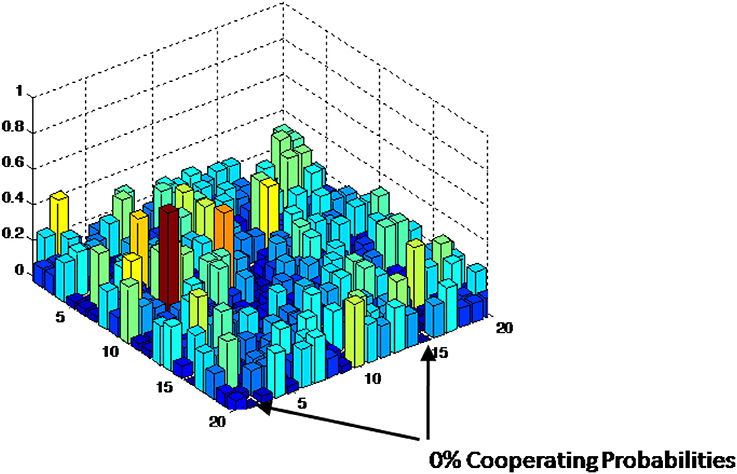
Figure 6. Agent cooperating probability with high negative S values.

2.3. Analysis of Zeros and Ones

In the previous section the transition between plateaus was evaluated and boundaries were created where the analytical solution and the simulation results were within a threshold 0.01. The selection of 0.01 as a tolerance was arbitrary and the selection of a boundary when S becomes highly negative was a best fit judgment insertion. Although this does represent cases where the analytical solution is close to simulation results, we will now present a different and more unique method to better depict where the solution is working without the use of arbitrary tolerances or judgments.

From the analyses above it was concluded that the solution works when agents' are bipartisan without any adjustments being made to any agent's cooperating probability. That is, their cooperating probability fluctuates around the steady state equilibrium and never has to be adjusted because it becomes greater than one or negative. It is evident from the derivation of the analytical solution that it does not account for any adjustments of the cooperating probabilities to one or to zero. It is also clear that in the plateaus and regions where the analytical solution doesn't work some or all of the agents' cooperating probabilities are being adjusted to zero or to one. So the idea is to look at the simulation run and determine the regions with no agents having a zero or unit cooperating probability. If there are no agents with a zero or unit cooperating probability, then their cooperating probabilities must fluctuate around a steady state value in the bipartisan region for which the analytical solution works.

In order to test this theory we ran a simulation where we counted the number of agents with zero or one cooperating probability at the end of the run. In this simulation R = 1 and P = −1, with T and S varying between −10 and 10. The simulation is run on a 50 × 50 cellular automaton grid with each Pavlovian agent having an initial cooperating probability 0.2 and equal learning factors 0.05. Figure 7 shows the results of this simulation. The right side graph shows the percentage of agents with zero cooperating probability and the left side graph shows the percentage of agents with unit cooperating probability. We will now look at various plateaus in order to interpret these simulation results.

FIGURE 7

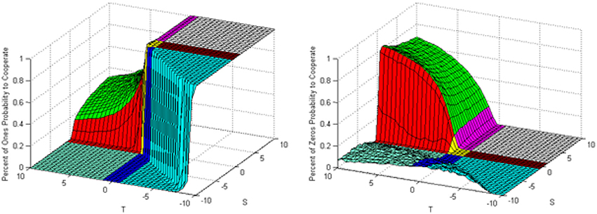
Figure 7. Percentage of agents with cooperating probabilities of one and zero during last iteration.

Consider first the Harmony/Deadlock Plateau where we have unison agents. From reviewing the graphs shown in Figure 7 we find that in this region (High Positive S, High Negative T) none of the agents have zero cooperating probability and 100% of the agents have unit cooperating probability. This is expected since all of the agents are cooperating in this region.

Now we look at the Leader/Battle of the Sexes Plateau where we have partisan agents. We see in Figure 7 that a certain percentage of the agents have unit cooperating probability, and the rest of the agents have zero cooperating probability. This is again expected as we have seen that in this plateau a portion of the agents cooperate with certainty and the rest defect with certainty.

Finally, in the Prisoners' Dilemma Plateau it is seen that none of the agents have a unit cooperating probability. We also see that the percentage of agents with a zero cooperating probability is minimal near S = 0 and increases as S becomes a larger negative number. This is again expected from the above analysis where agents are severely punished as S becomes a larger negative number, so some of the cooperating probabilities become negative and are adjusted to zero.

The area where the analytical solution works best is the region where there are no agents with zero cooperating probability and also no agents with unit cooperating probability. This is shown in bright green color in Figure 8. It is seen that the analytical solution works best in the Chicken/Prisoners' Dilemma region and also in parts of Stag Hunt and Coordination games.

FIGURE 8

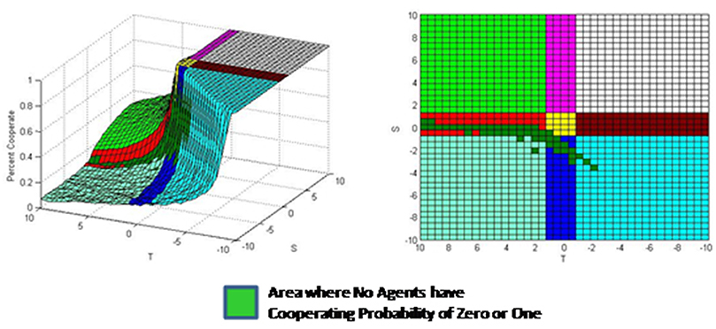
Figure 8. Area where simulation has no agents with cooperating probability of zero or one.

In order to expand the solution set, Figure 9 shows the simulation results for several values of R and P. From these results it is observed that the analytical solution actually works best in the Chicken game when S is slightly less than zero. This is somewhat surprising in comparison to the previous literature which has only referenced that the analytical solution is working in the Prisoner's Dilemma game.

FIGURE 9

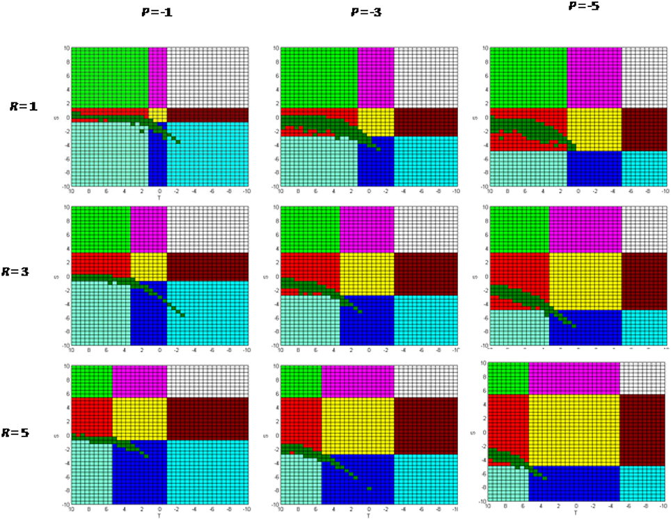
Figure 9. Simulation results with varying values of R and P.

3. Sensitivity Analysis and Impact of Variables

In sections 2.2 and 2.3 it was presented that the analytical solution becomes progressively worse in the Prisoners' Dilemma region as S becomes more negative. This is due to the fact that as S grows more negative the punishment for cooperation rises to the point where an agents cooperating probability by Equation (1) becomes negative and has to be adjusted to zero. This negatively impacts the quality of the analytical solution in the Prisoners' Dilemma game. The purpose of this section is to evaluate how sensitive the analytical solution is as S grows more negative and to evaluate the impact of changing the initial cooperating percentage. After that, the impact of changing other parameters will be explored including changing learning factors, allowing R and P to be either both positive or both negative, and changing neighborhood size.

Figure 10 shows the difference between the analytical solution and the simulation results for R = 1 and P = −1 with common learning factor 0.05 and initial cooperating probability 0.2. The figure shows that the analytical solution is working optimally when S is slightly less than zero in the Chicken region and becomes worse with values of S more negative and also with small value of T. The reason that the difference raises as T decreases in positive values is that the cooperating probability does not raise as much with a lower value of T and thus makes the agent's cooperating probability more susceptible to become negative on the next iteration when the agent should cooperate and be punished. This figure provides good detail on how much the analytical solution is degrading from the simulation results as well as where the difference is within the selected 0.01 tolerance. This figure shows that the analytical solution is only a good estimate in the Prisoner's Dilemma region which degrades as S becomes more negative or T becomes less positive.

FIGURE 10

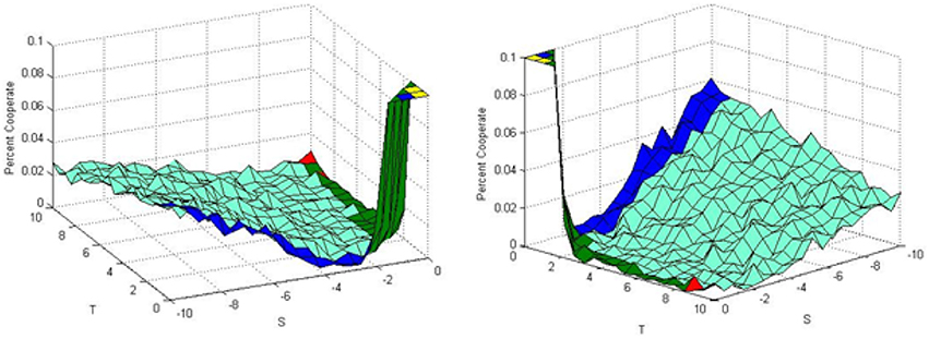
Figure 10. Difference between simulation and analytical solution when R = 1 and P = −1.

Other initial cooperating probabilities will now be evaluated in order to see if they are sensitive to the previous results. Figure 11 provides five specific simulations (labeled A, B, C, D, and E) with each simulation presenting several different initial cooperating probabilities. For example, the top left hand side plot has the parameter values R = 1, P = −1, T = 5, and S = −1 with initial cooperating probabilities 0.0, 0.2, 0.4, 0.6, 0.8, and 1.0. In these simulation results the red line is the analytical solution and the blue lines are the percentages of cooperators at each iteration given the different initial cooperating probabilities. The insert in each chart shows a magnified view in steady state condition for better comparison to the analytical solution. The five simulation cases in this figure differ from each other only in the value of S. The bottom right hand plot of Figure 11 shows the specific simulations depicted with white dots. It can be seen that the applicability of the analytical solution is not sensitive to the initial cooperating probability. The only exemption occurs when the initial cooperating probability is very high. In this case bipartisan behavior is not achieved as explained in Szilagyi [12]. The slow degradation of the analytical solution compared to simulation results can again be seen as S becomes larger negative.

FIGURE 11

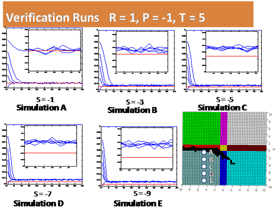
Figure 11. Simulation results for several initial cooperating probabilities with varying value of S.

Figure 12 shows the impact of lowering the values of the learning factors. This simulation is the same as the one shown in Figure 8 except that the learning factors are α = β = 0.01 instead of α = β = 0.05. It can be seen that the green area expands when the learning factors are lowered. This is because as the learning factors are lowered the cooperators have less punishment by Equation (1) in the Prisoner's Dilemma game with fixed S value. In essence, the agent's cooperating percentage will get closer to a steady state value when the learning factors are lowered thus making the analytical solution more applicable for wider range of S values.

FIGURE 12

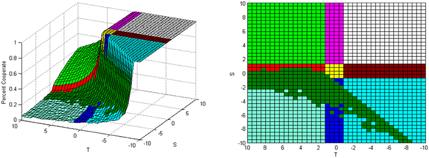
Figure 12. Simulation results with learning factors α = β = 0.01.

Up to this point we have assumed that reward is a positive payoff and punishment is a negative payoff. Figure 13 shows the simulation results for two cases when the reward R and punishment P values are both positive. In this case the bipartisan behavior in the Prisoner's Dilemma disappears and the analytical solution will not work for any S, T parameter values. This is shown in Figure 13 by the fact that all of the agents in the Prisoner's Dilemma plateau are defectors 100% of the time. In this region the agents' cooperating probabilities become negative and being adjusted to zero. Figure 14 shows the simulation results when the reward R and punishment P are both negative. In this case bipartisan behavior can occur in the Harmony/Deadlock plateau and the analytical solution applicability is expanded. The reason that the bipartisan behavior is expanded is not explained completely in the literature. This is an area for potential future research.

FIGURE 13

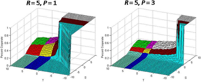
Figure 13. Simulation results with positive R and P values.

FIGURE 14

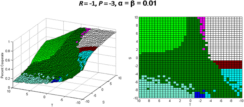
Figure 14. Simulation results with negative R and P values.

In all previous simulations we assumed that each agent is interacting with all agents as a whole. We will now look at the impacts of different neighborhood sizes on the applicability of the analytical solution. Figure 15 presents the simulation results using the same parameter values as those used in Figure 8 except with using the Moore neighborhoods of 1, 5, 10, and 50. The results show that the applicability of the analytical solution expands slightly when the neighborhood size increases. This difference can be explained by the fact that when the neighborhoods are in close proximity then their payoff values become more discreet making an agent's cooperating probability oscillate with higher values. For example, in unit neighborhood size there are only eight other neighbors plus the agent itself in the neighborhood. This means that there are only 10 possible percentages of the cooperating agents (0, 11, 22, 33, 44, 56, 67, 78, 89, and 100%) and thus there are only ten possible discrete payoff values. The values are slightly higher in this case because higher oscillation results in more instances when an agent's probability becomes negative per Equation (1) and it is artificially increased to zero. This periodic artificial upward adjustment in an agent's cooperating probability from a negative number to zero results in a slight raise in the percentage of cooperators in the system.

FIGURE 15

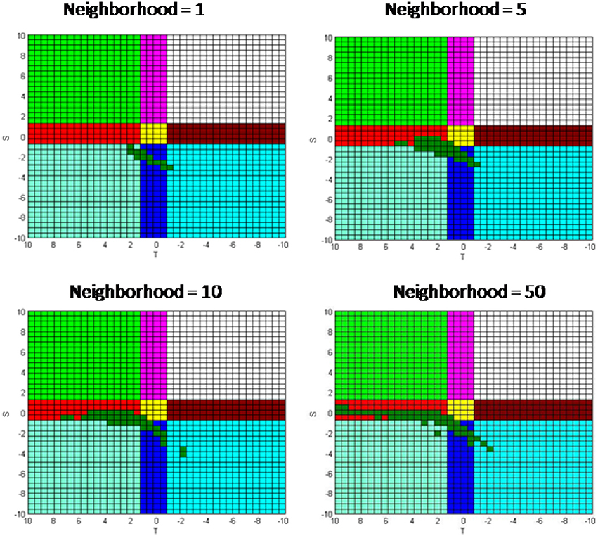
Figure 15. Simulation results with different neighborhood sizes.

4. Conclusions

This paper presented the applicability of the analytical solution of the N−person social dilemma game assuming Pavlovian agents with linear payoff functions in a two-dimensional cellular automaton environment.

A derivation of the analytical solution was given. A key assumption in this derivation is that the cooperating probability is continuous without the use of adjustments when the cooperating probability becomes negative or exceeds one. This derivation will not be applicable in scenarios where the cooperating probability for an agent is either consistently going negative and be adjusted to zero or going above one and being adjusted to one.

The behavior of the agents was reviewed. It was seen that there are three plateaus where agents act in different manners. The first plateau consists of predominately the Prisoners' Dilemma game where each agent's cooperating probability fluctuates around a steady state equilibrium. These agents are called bipartisan since they are willing to change their minds from iteration to iteration. The second plateau consists of a region consisting of the Leader and the Battle of the Sexes games where the agents decide to either cooperate or defect and then never change their minds. These agents are called partisan because of their reluctance to change their decision. The final plateau consists of the region including the Harmony and the Deadlock games where all agents decide to cooperate. These agents are called unison since they all make the same decision. The analytical solution is not effective for partisan and unison agents since their cooperating probabilities are consistently becoming negative or exceeding one and being adjusted.

It was determined with agent based simulation where the analytical solution is close to the simulation results. This region consisted of portions of the Prisoners' Dilemma, Chicken, Stag Hunt, and Coordination games. A characteristic of this region is that there are no or few agents with zero or unit cooperating probability. The area where the analytical solution closely approximates the simulation results was bounded by using agent behavior traits, but judgments and arbitrary tolerances were required to be used.

The area where the solution works optimally was determined without judgments and arbitrary tolerances using a special method. This method finds the area where no agents have a zero or unit cooperating probability in the final run. In this case the agents are systematically fluctuating around the steady state without having any cooperating probability adjustments to zero or one. It is seen that the analytical solution works optimally in the Chicken game where S is slightly negative and enters into Prisoner's Dilemma, Stag Hunt, and the Coordination games.

It was determined that the analytical solution degrades as S becomes more negative. A sensitivity analysis was performed using agent based simulation to assess this degradation in the Prisoners' Dilemma game, which was also repeated with different initial cooperating probabilities. The results confirmed the degradation of the analytical solution as S became more negative and indicated that the results are not sensitive to the initial cooperating probability.

The impact of the reward R and punishment P values being either both positive and both negative were explored. When they are positive the analytical solution does not work for any S,T value. This is because there is no bipartisan behavior in any region when both parameters are positive. When both the reward and the punishment are negative then the applicability of the analytical solution expands into the Harmony/Deadlock plateau as bipartisan behavior can exist in this region.

The impact of the learning factors and the neighborhood size were also evaluated. Lowering the value of the learning factors increases the applicability of the analytical solution for a given set of parameters in the Prisoner's Dilemma game because this reduces the punishment impact of Equation (1) and thus reduces the chance of an agent's cooperating probability becoming negative. Lower neighborhood sizes or close proximity neighborhood have smaller analytical solution applicability regions because few neighbors lead to more discrete payoff values which tend to cause higher fluctuations and thus more situation where an agent's cooperating probability becomes negative.

In this paper linear payoff functions and linear probability updating rules were considered. In our next project we will consider and analyze nonlinear models.

Author Contributions

UM: behavioral analysis and theoretical discussion; FS: formalization and theoretical discussion; DS: simulations.

Funding

The work has been developed in the framework of the research project on Dynamic Models for behavioral economics financed by DESP-University of Urbino.

Conflict of Interest Statement

The authors declare that the research was conducted in the absence of any commercial or financial relationships that could be construed as a potential conflict of interest.

References

1. Davidsson P. Multi agent based simulation: beyond social simulation. In: Moss S, Davidsson P, editors. Multi-Agent-Based Simulation. Cambridge, MA: Springer Berlin Heidelberg (2001). p. 141–55.

Google Scholar

2. Davidsson P. Agent based simulation: a computer science view. J Artif Soc Soc Simul. (2002) 5:1–7. Available online at: http://jasss.soc.surrey.ac.uk/5/1/7.html

Google Scholar

3. Epstein JM, Axtell R. Growing Artificial Societies: Social Science from the Bottom Up. Cambridge, MA: MIT Press (1996).

Google Scholar

4. Poundstone W. Prisoner's Dilemma. New York, NY: Doubleday (1992).

5. McAdams RH. Beyond the prisoners' dilemma: coordination, game theory, and the law. S Cal L Rev. (2009) 82:209–25. Available online at: https://ssrn.com/abstract=1287846

Google Scholar

6. Axelrod R, Keohane RO. Achieving cooperation under anarchy: strategies and institutions. World Polit. (1985) 38:226–54.

Google Scholar

7. Power C. A spatial agent-based model of N-Person Prisoner's dilemma cooperation in a socio-geographic community. J Artif Soc Soc Simul. (2009) 12:8. Available online at: http://jasss.soc.surrey.ac.uk/12/1/8.html

Google Scholar

8. Szilagyi MN. Cars or buses: computer simulation of a social and economic dilemma. Int J Int Enterpr Manage. (2009) 6:23–30. doi: 10.1504/IJIEM.2009.022932

PubMed Abstract | CrossRef Full Text | Google Scholar

9. Merlone U, Sandbank DR, Szidarovszky F. Equilibria analysis in social dilemma games with Skinnerian agents. Mind Soc. (2013) 12:219–33. doi: 10.1007/s11299-013-0116-6

CrossRef Full Text | Google Scholar

10. Merlone U, Sandbank DR, Szidarovszky F. Systematic approach to N-person social dilemma games: classification and analysis. Int Game Theor Rev. (2012) 14:1250015. doi: 10.1142/S0219198912500156

CrossRef Full Text | Google Scholar

11. Rapoport A, Guyer M. A taxonomy of 2 × 2 games. Gen Syst. (1966) 11:203–14.

Google Scholar

12. Szilagyi MN. An investigation of N-person Prisoners' Dilemmas. Complex Syst. (2003) 14:155–74.

Google Scholar

13. Thorndike EL. Animal Intelligence. Darien, CT: Hafner (1911).

PubMed Abstract | Google Scholar

14. Bush RR, Mosteller F. Stochastic Models of Learning. New York, NY: John Wiley & Sons (1955).

Google Scholar

15. Macy MW, Flache A. Learning dynamics in social dilemmas. Proc Natl Acad Sci USA. (2002) 99:7229–36. doi: 10.1073/pnas.092080099

PubMed Abstract | CrossRef Full Text | Google Scholar

16. Flache A, Macy MW. Stochastic collusion and the power law of learning. J Confl Resolut. (2002) 45:629–53. doi: 10.1177/002200202236167

CrossRef Full Text | Google Scholar