A Testing Method of Probability Weighting Functions From an Axiomatic Perspective

Introduction

A probability weighting function W(p) is a nonlinear function of an objective probability p, where p is determined primarily from the frequentist view. Recently, they have received substantial empirical and theoretical attention [1–3]. They are used in many fields, such as behavioral decision theory, behavioral economics and neuroscience [4].

Several psychometric models have been proposed to represent probability weighting functions (e.g., [1–3, 5, 6]). Some proposed probability weighting models derive from time discounting models [2, 3, 7]. Rachin et al. [7] derived the model from the original hyperbolic function. Takahashi [2] used a q-exponential time discount function [8] to derive Prelec's [6] probability weighting function and an exponential power model. Takemura and Murakami [3] used a more direct assumption of time discounting to derive the hyperbolic logarithmic function model and the generalized hyperbolic logarithmic model as probability weighting functions.

Takemura and Murakami [3] used a generalized hyperbolic time discounting model that assumes both Fechner's [9] psychophysical law of time and a geometric distribution of trials. From this, they derived hyperbolic logarithmic type models. They were then able to examine the generalized hyperbolic model in the context of an axiomatic system. They used Gonzalez and Wu's [10] procedure to estimate the function parameters. To investigate goodness of fit, they computed both the Akaike Information Criterion (AIC) and Bayes Information Criterion (BIC). The results indicated that the generalized hyperbolic logarithmic mode originally proposed by Prelec [6] fitted better than median time discounting models, the one-parameter Prelec model, and the Tversky and Kahneman model.

Takemura and Murakami [3] made a key contribution by supporting, both theoretically and empirically, a possible psychological interpretation of a probability weighting function in the context of time discounting. However, the empirical method used in the study was a psychometric nonlinear regression study. Although there are several empirical psychometric tests available to examine probability weighting functions, there is no concrete method to examine the axiomatic properties of the probability weighting functions. Prelec [6] had already proposed the axiomatic properties for some weighting functions. However, no concrete axiomatic properties distinguished the individual models he proposed, and no testing method was suggested. Based on their axiomatic considerations, we propose axiomatic properties and a testing method to examine the generalized hyperbolic logarithmic model, power model, and exponential power model of the probability weighting functions, and provide an illustrative example of the testing method.

Axiomatic System of Generalized Hyperbolic Logarithmic Model, Exponential Power Model, and Power Model for Probability Weighting Functions

Counterexamples, such as the Allais paradox [11] and the Ellsberg paradox [12], have been identified in earlier studies. These paradoxes are interpreted as deviations from the independence axiom. Recently, they have been explained using theory systems. More specifically, these systems include the nonlinear utility theory [13–15]—which does not require this independence axiom—as well as the generalized expected utility theory [16]. Prospect theory [5, 17] integrates knowledge and past findings in nonlinear utility theory (or generalized expected utility theory) and behavioral decision-making theory.

In prospect theory, we assume a non-additive probability function, where a non-additive probability is a set function π:2^Ω → [0, 1] from an aggregate of subsets of a nonempty set Ω to a closed interval [0, 1]. The non-additive probability function is a set function satisfying both a boundedness condition (π(ϕ) = 0, π(Ω) = 1) and a monotonicity condition [if A⊆B, then π(A) ≤ π(B), where A, B are subsets of Ω]. A non-additive probability does not necessarily satisfy additivity conditions. Prelec [6] showed psychometric functions of non-additive probability (probability weighting functions) and axiomatic properties of the probability weighting functions based on prospect theory.

Based on the theoretical work of Prelec [6], we show axiomatic properties of the generalized hyperbolic logarithmic model, exponential power model, and power model for probability weighting functions.

For the set A of probability distributions P, Q, … on X = [x⁻, x⁺], where x⁻ < 0 < x⁺, let ≽ be a preference relation. Prospects are considered distributions with finite support. Then, we assume the following axioms [6].

W1. Weak ordering: ≽ is complete and transitive.

W2. Strict stochastic dominance: P > Q if both P≠Q and P is stochastically dominants over Q.

W3. Certainty equivalent condition: For every P, ∃ x such that (x) ~ P.

W4. Continuity in probabilities: If (y, p) > (x) where 0 < p < 1, then ∃ q, r such that q < p < r, (y, q) > (x), and (y, r) > (x). If (y, p) < (x) where 0 < p < 1, then ∃ q, r such that q < p < r, (y, q) < (x) and (y, r) < (x).

W5. Simple continuity: Let the set of all k nonpositive and (n−k) nonnegative rank-ordered n-tuples from X be S(k, n), where 0 ≤ k ≤ n. If the preference relation induced on each set S(k, n) is continuous for any probability vector (p₁, p₂, ⋯, p_n), then there is simple continuity.

W6. Tradeoff consistency: Consider a prospect (x, p_i; x_−i, p_−i) with outcome c of rank i singled out and the set R(k, n, p) of all sign-order and rank-order compatible prospects with a p-chance of a negative outcome. Assume there are not eight prospects, (x, p_i; a_−i, p_−i), (y, p_i; b_−i, p_−i), $(x^{\prime },p_i;{\text{a}}_{-\text{i}},{\text{p}}_{-\text{i}})$, $(y^{\prime },p_i;{\text{b}}_{-\text{i}},{\text{p}}_{-\text{i}})$, $(x^{\prime },q_j;{\text{c}}_{-\text{j}},{\text{q}}_{-\text{j}})$, $(y^{\prime },q_j;{\text{d}}_{-\text{j}},{\text{q}}_{-\text{j}})$, (x, q_j; c_−j, q_−j), and (y, q_j; d_−j, q_−j), such that the first and second groups of four belong to the same sign-order and rank-order compatible set, and

$\begin{array}{lll}(x,p_i;{\text{a}}_{-\text{i}},{\text{p}}_{-\text{i}})& \succcurlyeq & (y,p_i;{\text{b}}_{-\text{i}},{\text{p}}_{-\text{i}}),\\ (x^{\prime },p_i;{\text{a}}_{-\text{i}},{\text{p}}_{-\text{i}})& \preccurlyeq & (y^{\prime },p_i;{\text{b}}_{-\text{i}},{\text{p}}_{-\text{i}}),\\ (x^{\prime },q_j;{\text{c}}_{-\text{j}},{\text{q}}_{-\text{j}})& \succcurlyeq & (y^{\prime },q_j;{\text{d}}_{-\text{j}},{\text{q}}_{-\text{j}}),\\ (x,q_j;{\text{c}}_{-\text{j}},{\text{q}}_{-\text{j}})& <& (y,q_j;{\text{d}}_{-\text{j}},{\text{q}}_{-\text{j}}).\end{array}$

Then, tradeoff consistency holds.

The following assumptions are as described by Prelec [6].

Assumption 1: ≽ satisfies axioms W1-W6, which support a sign-dependent and rank-dependent representation with a continuous and strictly increasing ratio scale v(x), as well as a strictly increasing unique w⁻(p), w⁺(p) that is continuous on (0, 1), and satisfies w⁺(0) = w⁻(0) = 0, w⁺(1) = w⁻(1) = 1.

Assumption 2: There is a separable representation of the restriction of ≽ to simple prospects, with v(x), w⁻(p), and w⁺(p) satisfying the Assumption 1 conditions.

Definition 1 Conditional invariance [6]: ≽ has conditional invariance if the following holds for any outcomes x, y, x′, y′ ∈ X, probabilities q, p, r, s ∈ [0, 1], and conditional probability λ, 0 < λ < 1:

If (x, p) ~ (y, q) and (x, r) ~ (y, s), then (x′, λp) ~ (y′,λq) implies (x′, λr) ~ (y′, λs) or (x′, λr) ~ (y′,λs).

Definition 2 Projection invariance [6]: ≽ has projection invariance if the following holds for any outcomes x, y∈X, probabilities q, p, r, s∈[0, 1], and conditional probability λ, 0 < λ < 1:

If (x, p) ~ (y, q) and (x, rp) ~ (y, sq), then (x, r²p) ~ (y, s²q).

Proposition 1: The generalized hyperbolic logarithmic model proposition

Let ≽ be a preference relation on R⁺ where either Assumption 1 or 2 holds, conditional invariance (Definition 1) does not hold, and projection invariance (Definition 2) holds. Then, the probability weighting function W(p) is a hyperbolic logarithm,

$\begin{array}{l}W(p)={(1-klogp)}^{\beta },\end{array}$

where p is probability (0 < p), and k and β are positive constants, k, β > 0.

Proof

The proof of Proposition 1 is trivial and derived from a combination of Propositions 4 and 5 in the original theoretical work by Prelec [6]. Prelec [6] found that if ≽ is a preference relation on R⁺ where either Assumption 1 or 2 holds and conditional invariance (Definition 1) holds, then the weighting function (0 < p) is either an exponential-power function or a power function (Proposition 4). Prelec [6] also found that if ≽ is a preference relation on R⁺ where either Assumption 1 or 2 holds and projection invariance (Definition 2) holds, then the weighting function (0 < p) is either a hyperbolic logarithm or a power function (Proposition 5). Therefore, if ≽ is a preference relation on R⁺ satisfying Assumption 1 or 2, conditional invariance (Definition 1) does not hold, and projection invariance (Definition 2) holds, then the probability weighting function W(p) is a hyperbolic logarithmic function.

Proposition 2: Proposition of the exponential power model

If ≽ is a preference relation on R⁺ satisfying Assumption 1 or 2, conditional invariance (Definition 1) holds, and projection invariance (Definition 2) does not hold, then the probability weighting function W(p) is an exponential power function such as

$\begin{array}{l}W(p)=exp\left\{-k(1-p^{\beta })\right\},\end{array}$

where p is probability (p > 0), and k and β are positive constants, k, β > 0.

Proof

The proof of Proposition 2 is trivial and also derived from a combination of Propositions 4 and 5 in the original theoretical work by Prelec [6]. As in the same inference of Proposition 1, if ≽ is a preference relation on R⁺ satisfying Assumption 1 or 2, conditional invariance (Definition 1) holds and projection invariance (Definition 2) does not hold, then the probability weighting function W(p) should be an exponential power function.

Proposition 3: Proposition of the power model

If ≽ is a preference relation on R⁺ satisfying Assumption 1 or 2, conditional invariance (Definition 1), and projection invariance (Definition 2), then the probability weighting function W(p) is an exponential power

$\begin{array}{l}W(p)=p^{\beta },\end{array}$

where p is probability, and β is a positive constant, β > 0.

Proof

The proof of for this proposition is trivial and also derived from a combination of Propositions 4 and 5 in the original theoretical work by Prelec [6]. As in the same inference of Proposition 1, if ≽ is a preference relation on R⁺ satisfying Assumption 1 or 2, conditional invariance (Definition 1) holds and projection invariance (Definition 2) holds, then the probability weighting function W(p) is a power function.

A Testing Method to Examine Axiomatic Properties of Generalized Hyperbolic Logarithmic Model, Exponential Power Model, and Power Model for Probability Weighting

We propose a testing method to examine the generalized hyperbolic logarithmic model, power model, and exponential power model of the probability weighting functions, and provide an illustrative example of the testing method. First, we present the testing method using verification tasks of projection invariance and conditional invariance. We then give an example verifying the reliability and axioms and showing the goodness of fit of the models.

Figure 1 illustrates the testing experimental process, which had participants choose one option from two gambles. To assess reliability, projection invariance and conditional invariance should be examined at least twice. Additionally, trials are done at least 30 times to stabilize the responses.

FIGURE 1

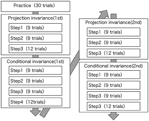
Figure 1. Experimental process for testing axiomatic properties.

The Projection Invariance Verification Process

Experimental screens and the task processes in the projection invariance verification process are shown in Figure 2. The task presented to the participants was to choose one option from two gambles as shown in Table 1. The participants were instructed to choose a preferred option from the experimenter.

FIGURE 2

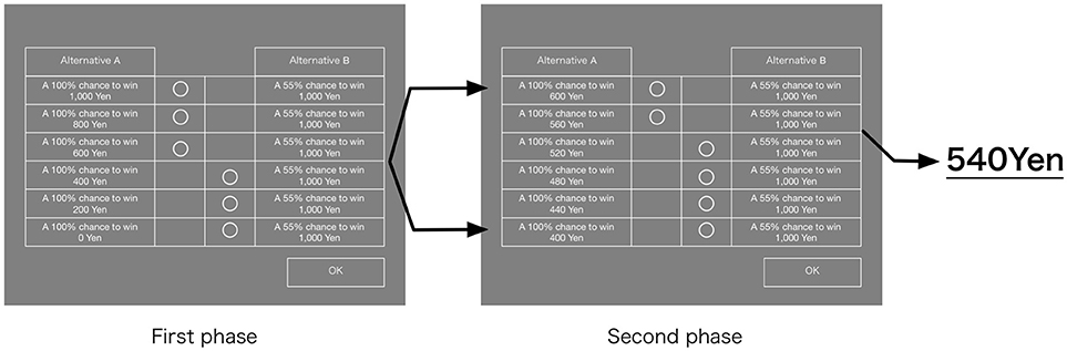
Figure 2. Experimental screens and task process.

TABLE 1

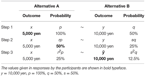
Table 1. Verification process of projection invariance.

The verification process of projection invariance is presented in Table 1. In the verification of projection invariance in Table 1, y = 10,000 yen, p = 100%, q = 50%, and s = 50% are given. In addition, Table 1 presents values of the responses by participants shown in bold typeface.

The verification projection invariance tasks comprise three steps. To explain the verification process using the example presented in Table 1, in Step 1, x in the alternative A equivalent to the alternative B (to obtain 10,000 yen with 50%) is estimated from a pair comparison of the alternative A and alternative B in Figure 2. Next, in Step 2, r in the alternative A equivalent to the alternative B (to obtain 10,000 yen with 25%) is estimated. For x of the alternative A in Step 2, the x obtained in Step 1 is used. Finally, in Step 3, using x and r obtained in Step 1 and Step 2, the alternative A (to get 5,000 yen with 25%) is made. Then ŷ is estimated (to obtain ŷ yen with 12.5%). Here, when ŷ obtained in Step 3 is 10,000 yen, which is the same as y, projection invariance is regarded as satisfied. Additionally, because y = 10,000 yen is given in Step 3, to estimate ŷ, 20,000 yen and 0 yen, respectively, the maximum value and the minimum value of ŷ were presented to the participants. Then they were asked to do the pair comparison, as shown in Figure 2.

Steps 1, 2, and 3 respectively comprise 9 trials, 9 trials, and 12 trials. The stimulation sequences used to verify projection invariance are shown in Table 2. Nine sequences of stimulation were prepared. Furthermore, because y is fixed at 10,000 yen in Step 3, when a participant gives a response to satisfy the axioms, the participant might continue to give the same response and is likely to change a response due to fluctuation of the psychological process. Therefore, with three sequences of dummy stimulation added to the nine sequences, Step 3 has 12 trials in all.

TABLE 2

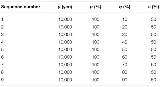
Table 2. Stimulation sequences of projection invariance.

Verification Process of Conditional Invariance

Experimental screens and task processes were prepared in an identical form to that used for projection invariance in the verification process of conditional invariance. The participants were also instructed to choose a preferred option from two gambles, as shown in Table 3. The verification process of conditional invariance is presented in Table 3. For verification of the conditional invariance in Table 3, y = 20,000 yen, y′ = 10,000 yen, p = 100%, q = 50%, s = 10%, and λ = 50% are given. Additionally, the values given in responses by the participants are shown in bold typeface in Table 3.

TABLE 3

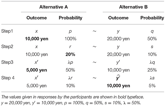
Table 3. Verification process of conditional invariance.

The verification tasks of conditional invariance comprise four steps. To explain the verification process using the example in Table 3, in Step 1, x of alternative A equivalent to alternative B (to get 20,000 yen with 50%) is estimated through a pair comparison between alternatives A and B as shown in Figure 2. Next, in Step 2, r of the alternative A equivalent to the alternative B (to get 20,000 yen with 10%) is estimated. For x of alternative A in Step 2, the x obtained in Step 1 is used. In Step 3, x′ of the alternative A (to obtain x′ yen with 50%) equivalent to the alternative B (to get 10,000 yen with 25%) is estimated. In Step 4, using r and x′ obtained in Step 2 and Step 3, respectively, alternative A (to get 5,000 yen with 10%) is made. Then, ŷ′ of alternative B (to get ŷ′ yen with 5%) is estimated. Here, when ŷ′ obtained in Step 4 is 10,000 yen, which is the same value as y′, the conditional invariance is regarded as satisfied.

Steps 1, 2, and 3 are composed respectively of 9 trials, 9 trials, and 12 trials. The stimulus sequences used for verification of conditional invariance are presented in Table 4. Nine sequences of stimuli were prepared. In Step 4, although three dummy stimulus sequences were also prepared for the same reason as those for projection invariance, three stimuli from the sequences were randomly provided twice because of the experimental program's errors. As a result, Step 4 had 9 sequences plus 3 trials, i.e., 12 trials in total.

TABLE 4

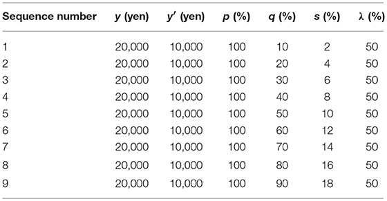
Table 4. Stimulus sequences of conditional invariance (%).

An Example of the Testing Method

Participants

The participants were 14 undergraduate students (eleven female and three male) studying psychology at Waseda University aged between 21 and 25 years old. They were paid 1500 Japanese yen (about 15 dollars) to participate in a 1.5-h test. This study has ethical approval from the Academic Research Ethical Review Committee, Waseda University concerning Guidelines Regarding Academic Research Ethics, Waseda University. Participants provided written informed consent.

Materials and Procedure

We asked the participants to select their preferred option from two alternatives while watching the screen shown in Figure 2. The verification procedure of projection invariance and conditional invariance were as described above.

Examination of Reliability

A participant was asked to work on the tasks twice in a row to assess the reliability. Intraclass correlation coefficients of projection invariance and conditional invariance by the participant was calculated. The intraclass correlation coefficients calculated from the first and second answers in the final step are shown in Table 5. Those calculated in all steps are shown in Table 6, with intraclass correlation coefficients that are 0.6 or greater presented in bold typeface. The medians of intraclass correlation coefficients calculated in the final step were 0.216 (maximum value, 0.871; minimum value, −0.324) in projection invariance and −0.131 (maximum value, 0.668; minimum value, −0.384) in conditional invariance. However, the medians of intraclass correlation coefficients calculated in all steps was 0.897 (maximum value, 0.992; minimum value, 0.401) in projection invariance and 0.765 (maximum value, 0.968; minimum value, 0.476) in conditional invariance.

TABLE 5

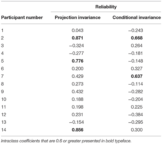
Table 5. Reliability of projection invariance and conditional invariance (final step).

TABLE 6

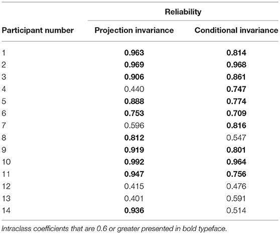
Table 6. Reliability of projection invariance and conditional invariance (all steps).

As Table 6 shows, the intraclass correlation coefficients are all 0.4 or greater for projection invariance and conditional invariance.

Verified Results of Projection Invariance and Conditional Invariance

Table 7 presents the numbers of sequences in which participants satisfied the axioms of projection invariance and conditional invariance. Because nine sequences were used to verify the axioms, when participants judge in accordance with the axioms in five sequences or more, the numbers are presented in bold typeface.

TABLE 7

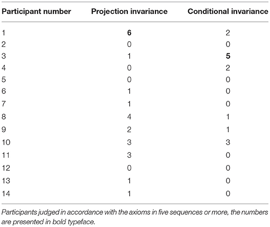
Table 7. Number of sequences satisfying the axiom (out of 9 sequences).

Examination of Goodness of Fit of the Model

Free parameters, such as β and k, of the probability weighting function by the participant were estimated by the same experiment as in Gonzalez and Wu [10]. Table 8 presents a list of examined models. In addition, Table 9 shows models which are the fittest according to AIC. Twelve participants had the best fit with the hyperbolic logarithmic model. One participant had the best fit with the exponential power function. One participant had the best fit with the power function.

TABLE 8

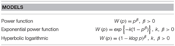
Table 8. List of models.

TABLE 9

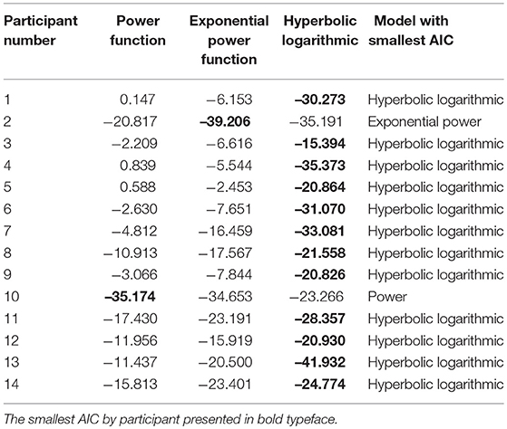
Table 9. Models' AICs and the model with the smallest AIC by participant.

Relation Between Axioms and Goodness of Fit of Models

The correspondence between axioms and models is presented in Table 10. Relations between satisfied axioms and models with goodness of fit are shown in Table 11. Because nine sequences were used to verify axioms, if axioms were satisfied in five and more sequences, then they are regarded as satisfied. The first participant satisfied projection invariance alone. The third participant satisfied conditional invariance. The other participants satisfied neither projection invariance nor conditional invariance. Results show that there is not a certain correspondence with normal quantitative psychometric methods that used the nonlinear regression method and the model fitting examination by AIC indicator.

TABLE 10

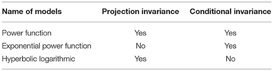
Table 10. Correspondence between axioms and models.

TABLE 11

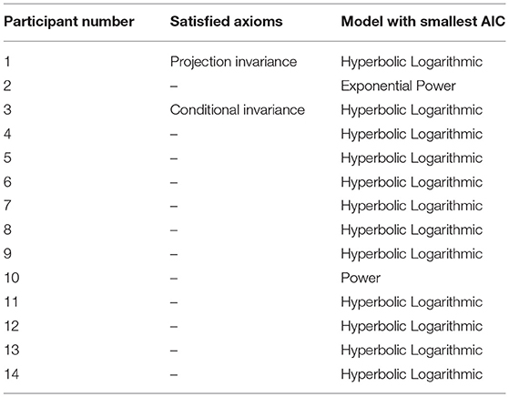
Table 11. Relations between satisfied axioms and models with goodness of fit.

Conclusion and Discussions

This study aimed to present a testing approach used to examine the generalized hyperbolic logarithmic model, power model, and exponential power model of the probability weighting functions that are considered nonlinear functions of probability in behavioral decision theory, for example, in prospect theory [6, 5]. Although many empirical psychometric tests are used to examine the probability weighting functions, there is no concrete method to examine the axiomatic properties of the probability weighting functions. Therefore, we propose axiomatic properties based on Prelec's [6] theory and a testing method to examine the generalized hyperbolic logarithmic model, power model, and exponential power model of the probability weighting functions, and provide an illustrative example of the testing method.

According to this result of the example experiment, the axiomatic properties of the probability weighting functions did not correspond to the psychometric fitting result of probability weighting functions. A similar result occurs in the additive conjoint systems in judgment and decision making. For example, empirical evaluations of double cancelation for the conjunctive measurement rejected the double cancelation axiom [18, 19]. However, psychometric studies have also indicated that the linear additive model fitted better [20]. There are some contradictions between psychometric studies and axiomatic studies. This case is the same as previous research. Further research is needed to identify why the discrepancies occur.

Luce and Steingrimsson [21] examined the Thomsen condition and the conjoint commutativity axiom, which they showed were equivalent. They also found that brightness and binaural loudness were supporting factors of conjoint commutativity. We must consider the reason for the unclear correspondence between the axiomatic testing and psychometric testing. One possibility is that the assumptions of the prospect theory did not hold in this experiment. Another is that the essential conditions, such as conditional invariance and projection invariance, did not hold in the experiment. Further research could investigate these possibilities.

In our study, the number of participants was limited and the participants were all trained psychology students. However, our sample size matches those in previous studies [5, 10], so we do not consider this to invalidate the results. Nevertheless, larger sample sizes in future experiments would be beneficial in examining the psychometric model of probability weighting functions.

Although we proposed an axiomatic testing method of Prelec's [6] probability weighting function, there other ways to interpret probability weighting, such as from the perspective of rational dynamic asset pricing theory. Rachev et al. [22] explained the main concepts of prospect theory and probability weighting functions within the framework of rational dynamic asset pricing theory. They derived a modified Prelec weighting function and introduced a new parametric class for weighting probability functions. We did not examine the theoretical notions proposed by Rachev et al. [22]. Further theoretical examinations are needed to seek an adequate probability weighting function.

Author Contributions

KT and HM developed the theoretical formalism, performed the analytic calculations and performed data analysis. Both authors contributed to the final version of the manuscript. KT supervised the project.

Funding

This study was supported by a Grant-in-Aid for Scientific Research (A), No. 24243061 and No. 16H02050 from The Ministry of Education, Culture, Sports, Science and Technology, Japan.

Conflict of Interest Statement

The authors declare that the research was conducted in the absence of any commercial or financial relationships that could be construed as a potential conflict of interest.

Acknowledgments

We sincerely thank Yuki Tamari, Takashi Ideno, Takayuki Sakagami, Yutaka Nakamura, Yiyun Shou and the referees of this journal for their helpful comments.

References

1. Dhami S. The Foundations of Behavioral Economic Analysis. Oxford: Oxford University Press (2016).

Google Scholar

2. Takahashi T. Psychophysics of the probability weighting function. Physica A Stat Mech Appl. (2011) 390:902–5. doi: 10.1016/j.physa.2010.10.004

CrossRef Full Text | Google Scholar

3. Takemura K, Murakami H. Probability weighting functions derived from hyperbolic time discounting: psychophysical models and their individual level testing. Front Psychol. (2016) 7:778. doi: 10.3389/fpsyg.2016.00778

PubMed Abstract | CrossRef Full Text | Google Scholar

4. Takemura K. Behavioral Decision Theory: Psychological and Mathematical Descriptions of Human Choice Behavior. Tokyo: Springer (2014).

Google Scholar

5. Tversky A, Kahneman D. Advances in prospect theory: cumulative representation of uncertainty. J Risk Uncertainty (1992) 5:297–323. doi: 10.1007/BF00122574

CrossRef Full Text | Google Scholar

6. Prelec D. The probability weighting function. Econometrica (1998) 66:497–527. doi: 10.2307/2998573

CrossRef Full Text | Google Scholar

7. Rachlin H, Logue AW, Gibbon J, Frankel M. Cognition and behavior in studies of choice. Psychol Rev. (1986) 93:33–45. doi: 10.1037/0033-295X.93.1.33

CrossRef Full Text | Google Scholar

8. Cajueiro DO. A note on the relevance of the q-exponential function in the context of intertemporal choices. Physica A (2006) 364:385–8. doi: 10.1016/j.physa.2005.08.056

CrossRef Full Text | Google Scholar

9. Fechner GT. Elemente der Psychophysik. Leipzig: Breitkopf & Härtel (1860).

Google Scholar

10. Gonzalez R, Wu G. On the shape of the probability weighting function. Cognitive Psychol. (1999) 38:129–66. doi: 10.1006/cogp.1998.0710

PubMed Abstract | CrossRef Full Text | Google Scholar

11. Allais M. Le comportement de l'homme rationnel devant le risque; critique des postulats et axiomes de l'ecole Americaine. Econometrica (1953) 21:503–46.

Google Scholar

12. Ellsberg D. Risk, ambiguity, and the savage axioms. Q. J. Econ. (1961) 75:643–69 doi: 10.2307/1884324

CrossRef Full Text | Google Scholar

13. Fishburn PC. Nonlinear Preference and Utility Theory. Sussex: Wheatsheaf Books (1988).

Google Scholar

14. Edwards W. Utility Theories: Measurements and Applications. Boston: Kluwer Academic Publishers (1992).

Google Scholar

15. Starmer C. Developments in non-expected utility theory: The hunt for descriptive theory of choice under risk. J. Econ. Lit. (2000) 38:332–82. doi: 10.1257/jel.38.2.332

CrossRef Full Text | Google Scholar

16. Quiggin J. Generalized Expected Utility Yheory: The Rank-Dependent Model. Boston: Kluwer Academic Publishers (1993).

Google Scholar

17. Kahneman D, Tversky A. Prospect theory: an analysis of decision under risk. Econometrica (1979) 47:263–92. doi: 10.2307/1914185

CrossRef Full Text | Google Scholar

18. Levelt WJM, Riemersma JB, Bunt AA. Binaural additivity of loudness. Br J Mathemat Statist Psychol. (1972) 25:51–68. doi: 10.1111/j.2044-8317.1972.tb00477.x

PubMed Abstract | CrossRef Full Text | Google Scholar

19. Gigerenzer G, Strube G. Are there limits to binaural additivity of loudness? J Exp Psychol Hum Percept Perform. (1983) 9:126–36. doi: 10.1037/0096-1523.9.1.126

PubMed Abstract | CrossRef Full Text | Google Scholar

20. Dawes RM. The robust beauty of improper linear models in decision making. Am Psychol. (1979) 34:571–82. doi: 10.1037/0003-066X.34.7.571

CrossRef Full Text | Google Scholar

21. Luce RD, Steingrimsson R. Theory and tests of the conjoint commutativity axiom for additive conjoint measurement. J Mathemat Psychol. (2011) 55:379–89. doi: 10.1016/j.jmp.2011.05.004

CrossRef Full Text | Google Scholar

22. Rachev S, Fabozzi FJ, Racheva-Iotova B. Option pricing with greed and fear factor: the rational finance approach. arxiv [preprint] arXiv:1709.08134.