Comparison of Cross-Correlation and Joint-Recurrence Quantification Analysis Based Methods for Estimating Coupling Strength in Non-linear Systems

Introduction

Networks can usefully characterize a wide range of natural systems, including climate systems [2–5], ecological systems [6, 7], social systems [8], and neurological systems [9–12]. Properties of network representations of these systems often correspond to important features, including system susceptibility to perturbations or control [13, 14], capacity of individual elements or communities of elements to influence or be influenced [15], and the predicted propensity of systems to couple and exchange information [16–18]. However, to create a network representation of a system, the interaction or connectivity of the nodes (i.e., the individual elements that are being modeled) must be measured [19]. This process is not without its challenges, as measuring interactions between real-world systems can be difficult.

Many studies that assess network structure in multivariate time series data rely on linear methods like cross-correlation to assess interactivity [20]. However, real-world systems are frequently complex and non-linear, and consequently exhibit non-stationarity and unpredictable dynamics [21–25]. Additionally, signals may be contaminated with non-stationary changes in large scale structure or background noise (e.g., [26]). These properties can result in inaccurate estimations of coupling strength when using common linear methods for assessing statistical dependence [10, 27]. For instance, relying on cross-correlation to determine coupling between non-stationary systems can be misleading if the systems exhibit autocorrelation [4], as slow variation in the signals can cause large covariances between them even if there are no true interdependencies. Additionally, cross-correlation relies on variation around a location parameter (i.e., the mean of the time series), which may cause problems if there is more than one such location (e.g., a system with multiple basins of stability) or if there is no persistent central point.

Recently, Bashan et al. [1] developed an approach to deal with these limitations in cross-correlation by evaluating the temporal stability of cross-correlations between signals, rather than relying solely on the magnitude of correlation. The method, termed time-delay stability analysis (TDS), relies on the general observation that stable coupling relationships between systems transfer fluctuations from one system to another at a consistent time lag. Specifically, when time series are segmented into windows and cross-correlation is calculated over a range these intervals, long contiguous intervals during which the cross-correlation reaches a maximum magnitude at a consistent delay correspond to periods of strong coupling. This approach is similar to that of estimating phase between oscillators [28] as it indexes coupling strength through the consistency of temporal relationships between signals rather than the magnitude of their structural similarity. However, though Bashan and colleagues showed how TDS can overcome limitations associated with naïve cross-correlation, an outstanding question is whether this method can be improved with techniques that are inherently more robust to non-stationarity than cross-correlation, such as recurrence-based methods. For example, joint recurrence quantification analysis (JRQA), a multivariate extension of recurrence quantification analysis (RQA; [29, 30]), is a robust non-linear technique for assessing relationships in multivariate systems and has been used to study coupling between systems of qualitatively different dynamics [29, 31, 32].

In the present work, we compare two different instantiations of the TDS method, one based on cross-correlation and another based on JRQA. We also modify JRQA by applying a weighting factor to its output to ensure measures are proportional to the degree of truncation that occurs as a result of calculating similarities between time lagged signals. We extend TDS by introducing a new variable that is conceptually similar to the RQA variable MAXLINE—a measure of dynamic stability in recurrence quantification analysis [29]—and show how TDS metrics can be used to index coupling between systems of non-linear oscillators with different intrinsic characteristics, as well as coupling in multivariate signals obtained from pairs of people engaged in a verbal problem solving task. We use the TDS metrics from the interpersonal data to create graphs that we then summarize with a simple network metric (the number of edges) to show how restricting hand movement during conversation alters the global properties of networks depicting important aspects of interpersonal coordination.

TDS

Bashan et al. [1] introduced TDS as a method for determining coupling between complex signals based on cross-correlation. Broadly, TDS works by segmenting each signal from a set of multivariate time series data into overlapping windows and then conducting bivariate cross-correlation analyses between all pairwise combinations of the signals for each of the windows. Specifically, for each window, TDS begins by measuring the delay at which the absolute value of the cross-correlation between two signals achieves a maximum. The process is iterated over sliding windowed segments of the time series, and the result is a time series of delays indexing the temporal relationship between the signals. This time series is then summarized to yield the percentage of contiguous time series segments with similar temporal relationships between the systems being analyzed, which is termed Percentage Time Delay Stability (%TDS). Specifically, to calculate %TDS, each time series is first transformed, e.g., by aggregation, so that each signal has identical sampling rates and number of samples, N. Then, for each pair-wise comparison between signals, the two time series of length N are windowed into segments of length L with an advance of a, which results in a total of $N_L=\left(\frac{N-L}{a}+1\right)$ windows. For each segment, s, the signals are normalized to zero mean and unit variance (to remove large-scale trends and obtain dimensionless units) and their cross-correlation is calculated for a range of delays, τ,

$\begin{array}{ll}{c}_{xy}^s(\tau )={\displaystyle \frac{1}{L}{\sum }_{i=1}^L{x}_{i+(s-1)a}^s{y}_{i+(s-1)a+\tau }^s,}& (1)\end{array}$

where s is the segment being evaluated. The delay associated with the maximum absolute value of the cross-correlation within each segment is calculated as

$\begin{array}{ll}{\tau }_0^s={\displaystyle \tau {|}_{\left|C_{xy}^s(\tau )\right|\ge \left|C_{xy}^s({\tau }^{\prime })\right|\forall {\tau }^{\prime }}.}& (2)\end{array}$

The resultant sequence of ${\tau }_{0s=1,\dots ,N_L}^s$ is a time series representing the temporal relationship between two signals. Long sequences of τ₀ that do not fluctuate beyond a given threshold correspond to times of consistent temporal relationships and thus strong coupling. %TDS is then calculated as the percentage of total windows in ${\tau }_0^s$ of length N_τ0 for which no more than a set number of values of τ₀ fluctuate more than Δ_τ0 seconds. When calculating %TDS, Bashan et al. [1] set their parameters to N_τ0= 5 and Δ_τ0= 1 and required that at least 4 windows be within Δ_τ0 for a segment to be labeled stable, meaning that for each five segments of ${\tau }_0^s$, a section of segments was deemed stable if the maximum difference in the values of four of the segments was no more than 1 s. We note that this approach can result in an inflationary bias in the number of sections identified as stable, since particular subsets of stable indices can be counted twice (i.e., if the second through fifth segments fit the stability criteria, then with a sliding window of one, in the next window, the first four segments would also be labeled stable). In the present work, we compared only against the first segment of a window, meaning that if any three of the remaining four segments were within ±Δ_τ0 of the first segment in a window, then that segment was labeled as stable. %TDS was then calculated as the ratio of stable segments to the total number of segments evaluated, multiplied by 100.

JRQA

Recurrence quantification analysis (RQA), the method underlying JRQA, is a tool for measuring patterning and regularity in potentially non-linear or non-stationary time series [29, 30, 33]. RQA depends upon the construction of a recurrence matrix (R), usually obtained by identifying similar points in a time series by thresholding neighborhoods around points in a reconstructed phase-space,

$\begin{array}{ll}{R}_{ij}=\Theta \left(ϵ-\Vert {\vec{x}}_i-{\vec{x}}_j\Vert \right),i,j=1,\dots ,N,& (3)\end{array}$

where N is the number of observed points, ϵ is a similarity threshold and ${\vec{x}}_i$ and ${\vec{x}}_j$ are vectors locating the system in phase-space, || || is a norm, and Θ (·) is the Heaviside function, such that Θ(x) = 0 if x < 0 and Θ(x) = 1 otherwise. The similarity threshold, ϵ, is a parameter that determines whether vectors in the phase space are identified as recurrent, i.e., as revisiting the same area of the phase space. Choosing an appropriate value for ϵ can be difficult [34] and investigating the impact of ϵ on RQA output is an active research topic [35, 36]; in the present work, we use a nearest neighbor approach that does not require an explicit ϵ to be set.

While RQA was originally introduced to evaluate single systems, it has been extended in several ways to evaluate aspects of similarity in multiple systems, including cross-recurrence quantification analysis—a method for measuring structural similarities in phase space trajectories that requires the same dimensionality between the compared systems [27, 37, 38]—and joint-recurrence quantification analysis (JRQA), which can estimate temporal coupling between systems of different dimensionality [31]. In its simplest form, JRQA quantifies joint-recurrence as the tendency of different systems, X and Y, to revisit areas in their respective phase spaces at the same time (i.e., it quantifies the probability that recurrences are present at the same locations in the recurrence matrices for each of the systems compared). This in turn can be used to assess different types of synchronization between systems [32]. Joint-recurrence (JR) is calculated from the Hadamard product of two R's,

$\begin{array}{l}J{R}^{XY}\left({ϵ}_x,{ϵ}_y\right)={\displaystyle \frac{1}{N^2}{\sum }_{i,j=1}^N\Theta \left({ϵ}_x^i-\Vert {\vec{x}}_i-{\vec{x}}_j\Vert \right)}\\ \times \Theta \left({ϵ}_y^i-\Vert {\vec{y}}_i-{\vec{y}}_j\Vert \right),i,j=1,\dots ,N,& (4)\end{array}$

where XY denotes that JR is obtained from systems X and Y using ${ϵ}_x^i$ and ${ϵ}_y^i$ as similarity thresholds for the different systems and the index i denotes that the thresholds are potentially different for each point in the phase space (i.e., as would be the case in a nearest neighbor approach). JRQA can be conducted from R's obtained by finding a fixed number of nearest neighbors (i.e., 5% of possible neighbors) for all points [29]. However, this approach will often result in asymmetric R's. For example, a distal point a in the phase space can have a nearest neighbor b that in turn does not have a as one of its own nearest neighbors. This loss of symmetry means some network measures become more difficult to interpret [39] and also results in loss of computational efficiency, which is problematic because JRQA is much more computationally intensive than cross-correlation. To address this, we symmetrized R by obtaining the logical matrix (R+R^T) > 0, where R^T is the transpose of R. This assures both that each point has a minimum number of neighbors and that the recurrence matrix is symmetric. More refined methods exist to induce symmetry in Rs obtained via a modified nearest neighbor method (e.g., [40, 41]), but the approach taken here has the advantage of being comparatively simple. Once symmetry is imposed, JRQA can be conducted on the upper triangular portion of the Rs, which can save significant computational time.

Importantly, JRQA has been generalized to account for time-lags in the coupling between two systems [5, 32] and also to account for differing base recurrence rates [5, 32]. To modify JRQA to account for time delays between systems, a delay parameter τ can be added to the calculation,

$\begin{array}{l}J{R}_{\tau }^{XY}\left({ϵ}_x,{ϵ}_y\right)={\displaystyle \frac{1}{{N^{\prime }}^2}{\sum }_{i,j=1}^{N^{\prime }}\Theta \left({ϵ}_x^i-\Vert {\vec{x}}_i-{\vec{x}}_j\Vert \right)}\\ \times \Theta \left({ϵ}_y^{i+\tau }-\Vert {\vec{y}}_{i+\tau }-{\vec{y}}_{j+\tau }\Vert \right),\\ i,j=1,\dots ,N-\tau ,& (5)\end{array}$

in which N′ = N − τ and $\vec{y}$ is shifted by τ units. This analysis can capture the propensity of recurrences in X to precede recurrences in Y. The complimentary analysis of $J{R}_{\tau }^{YX}$ is obtained by interchanging the appropriate terms in equation 5, and the two series can be concatenated after multiplying the resultant $J{R}_{\tau }^{YX}\tau$ index by −1. However, there are two important consequences for JRQA that arise as a result of truncating time series by τ. First, since JRQA is a statistical method, less confidence is obtained with smaller samples compared to larger ones [29]. Second, as truncation increases, the recurrence plots become smaller and thus more influenced by points close the diagonal. These points may in turn be dominated by tangential, rather than recurrent, motion in the systems. This is often corrected by applying a “Thieler window” to regions close to main diagonal in R's, where “close” is often defined by the decorrelation time of the time series determined by either autocorrelation or average mutual information [29, 42]. Here, we modified $J{R}_{\tau }^{XY}$ by applying a weight to each value of τ proportional to the degree of truncation,

$\begin{array}{ll}J{R}_{{\tau }_w}^{XY}=J{R}_{\tau }^{XY}\frac{\left(\frac{{N^{\prime }}^2-N^{\prime }}{2}\right)}{\left(\frac{N^2-N}{2}\right)}.& (6)\end{array}$

In the present work, we combine the TDS method with JRQA and look for the value of τ for which the concatenated values of $J{R}_{{\tau }_w}^{XY}$ and $J{R}_{{\tau }_w}^{XY}$ obtains a maximum between systems for each time series segment s. These values are entered into TDS in the same way as τ in the cross-correlation analysis described above. For all analyses, we conduct JRQA with a fixed number of nearest neighbors (either 2.5% or 5%)—with neighbors obtained after applying a Theiler window equal to the decorrelation time of the time series determined by the average mutual information method—and apply Equation 6.

Data

Non-linear Oscillators—The Rössler System

To evaluate the ability of the cross-correlation and JRQA-based methods of TDS to accurately estimate the degree of coupling between different systems, we applied both to data derived from several coupled instantiations of the Rössler system over a range of different intrinsic characteristics and coupling strengths. The Rössler system is a non-linear oscillator capable of exhibiting a range of dynamic responses, including fixed point behavior, periodicity, and chaos, and it has been previously used as a proof of concept of JRQA [31, 32]. We used the following set of differential equations to specify the system,

$\begin{array}{l}\stackrel{.}{x_1}=-\left(1+\nu \right)x_2-x_3+k\left(y_1-x_1\right)\\ \stackrel{.}{x_2}=\left(1+\nu \right)x_1+a_1{x}_2\\ \stackrel{.}{x_3}=0.2+x_3(x_1-10)\\ \stackrel{.}{y_1}=-(1-\nu )y_2-y_3+k\left(x_1-y_1\right)\\ \stackrel{.}{y_2}=(1-\nu )y_1+a_2{y}_2\\ \stackrel{.}{y_3}=0.2+y_3(y_1-10),& (7)\end{array}$

where ν is a frequency detuning term, a₁ and a₂ are free parameters, and k is a diffusive coupling term that determines the interaction strength between the two oscillators [31]. The system was integrated using the MATLAB ode45 integrator (MathWorks, Natick, MA) with a time-step of 0.01 for 560 s (the first 200 s were removed to allow transitions, leaving 360 s of data). In all simulations, the coupling parameter was set to 0 for time 0–180 s (after the first 200 s were removed) and to k for times >180 s (i.e., the coupling was “switched on” halfway through the integration). These data were downsampled by a factor of 10 for a final sample rate of 10 Hz. We varied the detuning parameter ν from 0 to 0.04 in increments of 0.02, resulting in three values of this parameter. The coupling parameter k was varied between 0 and 0.2941 in increments of 0.0118, resulting in 26 values of this parameter. We evaluated 3 cases for each parameter setting: two Rössler systems in a phase-coherent regime (a₁ = a₂ = 0.15); one Rössler in a phase-coherent regime and one in the funnel regime (a₁ = 0.2925; a₂ = 0.15); and both Rössler systems in the funnel regime (a₁ = a₂ = 0.2925). For each comparison, we independently simulated 108 systems using randomized initial conditions for the six system coordinates sampled from a uniform distribution ranging from zero to one, for a total of 25,272 instantiations of the Rössler system.

In computing TDS, we set the window size to 48 s with a 4.8 s advance. For JRQA, delay embedding was not used; rather, all three dimensions from each system were used to calculate their respective recurrence matrices. Within each window, we calculated TDS using both JRQA (conducted with a fixed number of nearest neighbors set to 2.5%) and cross-correlation, resulting in a time series τ₀ for both JRQA (${\tau }_0^{jr}$) and cross-correlation (${\tau }_0^c$). These values were evaluated for %TDS using a window size of 5, and a threshold of 1 s. If four out of five consecutive values of τ₀ were within 1 s from the first time point in the segment, that segment was considered stable. To allow for transitions, only the last 19 segments of the coupled and uncoupled portions of the time series were entered into summary statistics (i.e., averaged values of %TDS were calculated from between 91.20 and 177.60 s for the uncoupled sections and between 268.80 and 355.20 s for the coupled sections; Figures 1, 2 below).

FIGURE 1

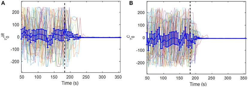
Figure 1. (A) τ₀ time series for 36 Rössler systems in the phase coherent regime with randomized initial conditions using JRQA-based TDS (${\tau }_0^{jr}$) with ν set to 0.04 and k set to 0.15. The time starts at 48 s as this is the last time point in the first TDS window (with a window size set to 48 s with a 4.8 s advance). The dotted black line marks the time coupling was initiated between the systems. Different instantiations of the systems are represented by different colored lines; the dark blue line is the mean and the error bars are 95% confidence intervals. (B) The same systems evaluated with cross-correlation-based TDS (${\tau }_0^C$).

FIGURE 2

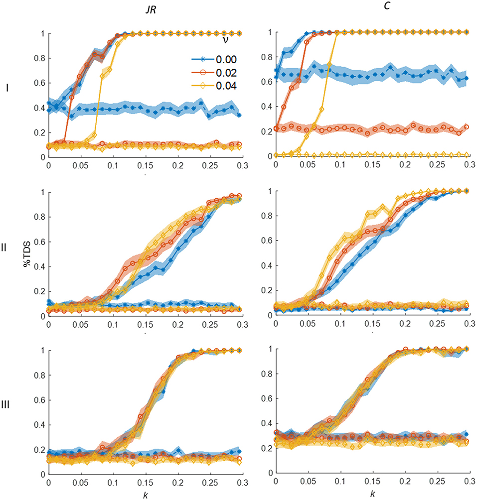
Figure 2. Mean values of %TDS results from analyses of Rössler systems as a function of phase-regimes, coupling strength k, and detuning factor, ν for JRQA-based (JR; left column) and cross-correlation-based analyses (C; right column). Row I: Two phase-coherent Rössler systems. Row II: One phase-coherent and one funnel regime system. Row III: Two funnel regime systems. For all figures, dashed lines (usually lower) indicate %TDS for uncoupled systems and the solid lines (usually higher) mark %TDS for systems after coupling is established. The shaded regions correspond to 95% confidence intervals obtained via a bias-corrected percentile bootstrap with 500 resamples.

Results of the Analyses of the Rössler System

Example time series of ${\tau }_0^{jr}$ and ${\tau }_0^C$ for a coupling strength of k = 0.15 from 36 iterations of Rössler systems with both systems in the phase-coherent regime can be seen in Figure 1. The effect of the onset of the coupling after 180 s (indicated by the dashed lines) is apparent, as is a transition to a stable interaction following the coupling onset.

Figure 2 shows the mean values of %TDS in the last 19 segments of the ${\tau }_0^{jr}$ and ${\tau }_0^C$ time series in the coupled and uncoupled systems for all parameters; shaded regions correspond to 95% confidence intervals calculated with a bias-corrected percentile bootstrap with 500 resamples. There are some notable differences in the results obtained from the two methods, in that TDS based on cross-correlation is often slightly more sensitive to coupling strength, with a steeper response in %TDS as a function of this parameter in phase-coherent to phase-coherent and funnel regime to phase-coherent systems (rows I and II in Figure 2). There is also a higher degree of separation between these signals in %TDS obtained from cross-correlation compared to %TDS obtained from JRQA as a function of the detuning parameter, ν. However, for all comparisons, the qualitatively similar response in %TDS for both JRQA-based and cross-correlation-based approaches is clear.

Interpersonal Dynamics

To test the ability of these methods to detect coupling in noisy, non-stationary data, we re-evaluated data collected by Tolston et al. [43]. In that experiment, dyads of randomly paired individuals were asked to complete visual puzzles by communicating with each other to uncover differences in their respective pictures when they could neither see their partner nor their partner's picture. The experimental manipulation was a repeated measures restraint placed on the hand movements of neither participant, one participant, or both participants. This resulted in two symmetric conditions in which both participants were either free to move their hands (free-free; FF) or both had their hand movements restrained (restrained-restrained; RR), and one asymmetric condition in which one participant was free to move his or her hands while the other participant's hands were restrained (free-restrained; FR). As expected, Tolston and colleagues found that the asymmetric condition resulted in significantly decreased similarities in postural dynamics measured using cross-recurrence quantification analysis (CRQA) at the waist, head, and hand, whereas the stability of joint attention measured using CRQA was highest when both participants were free to move their hands. However, the previous study was limited by the requirement of CRQA that the dimensionality of the phase-spaces of the systems being compared were identical, preventing comparison between different modalities (e.g., between gaze and postural dynamics). In the present analyses, we used the TDS framework to evaluate the stability of temporal relationships between different modalities of the participants, including waist, head, hand, gaze, and speech patterns. Details of the study can be seen in Tolston et al. [43], but we briefly describe the experimental procedure below.

The task consisted of finding differences in picture-puzzle pairs, with each puzzle pair being visually identical except for 10 differences. Participants were able to see one picture from each pair but were unable to see their partner or their partner's complementary picture. For each of their nine trials (3 in each restraint condition), participants had 190 s to find differences in their pictures by conversation. Prior to completing any puzzles, participants were equipped with magnetic motion trackers, head-mounted eye-trackers, and Bluetooth headphones. Postural data was sampled from the waist, head, and right hand from each participant. Pre-processing of the movement and gaze data is described in Tolston et al. [43]. Information about the pre-processing of the speech data is presented in Appendix A. For the present analyses, all data were analyzed at a sampling rate of 30 Hz, with a 30 s window and a 3 s advance. After processing all data, 14 pairs of dyads had full data sets. A variation of RQA maxline [29], TDSLMAX, was calculated as the longest stable sequence of τ₀. %TDS and TDSLMAX were calculated and then averaged for each pair in each condition, for a total of 14 observations in each condition. Due to a lognormal distribution, TDSLMAX was log transformed by adding one and taking the natural logarithm of the TDSLMAX values. For phase space reconstruction in support of JRQA [29], delays for the waist, head, and hand were each set to 63 samples with an embedding dimension of six. Delays for speech and gaze data were set to 30 samples, with an embedding dimension of four and six, respectively. Gaze data were embedded using a multidimensional method [44, 45], where horizontal and vertical gaze trajectories were embedded in the same space for a total of 12 dimensions in the reconstructed phase-space. For all of these analyses, JRQA was conducted with a fixed number of nearest neighbors set to 5%.

Surrogate Analyses

To evaluate the degree of interpersonal coupling in the different conditions, surrogate analyses were conducted for each of the three conditions by randomly selecting 100 surrogate pairings between virtual partners in the same condition (i.e., individuals who participated in the study but did not compete the task together) and calculating %TDS and TDSLMAX. These 100 values were then compared against the actual pairs using a one-tailed percentile bootstrap with 5,000 bootstrap samples [46] testing the null that the mean value of participant data was less than or equal to the mean value of the surrogate data (α = 0.05). These p-values were corrected using the false discovery rate correction [47]. Due to variations in network topology as a function of the similarity threshold, calculations are reported from the aggregation of a range of this parameter between 0.50 and 15s in increments of 0.50 s.

Results of the Analyses of the Tolston et al. Interpersonal Data

The number of significant links per condition as a function of Δ_τ0 and evaluation method for %TDS can be seen in Figure 3 and for TDSLMAX in Figure 4. Summary plots of the mean values for %TDS and TDSLMAX can be seen in Figure 5.

FIGURE 3

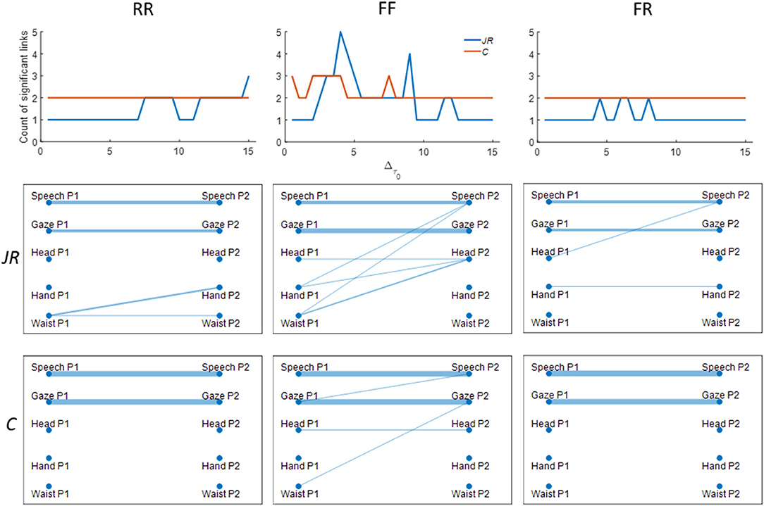
Figure 3. Figures summarizing graph density and topology for interpersonal data calculated using %TDS. Columns correspond to the three levels of hand restraint placed on the interacting pairs. The first row shows the count of significant links as a function of the TDS similarity threshold (Δ_τ0) for both JRQA-based and cross-correlation-based measures. The second and third row are networks showing the significant links between person one (P1) and person 2 (P2) identified by the JRQA-based and cross-correlation-based methods. The thickness of the lines in the graphs indicate the proportion of times that link was identified as significant over all values of Δ_τ0.

FIGURE 4

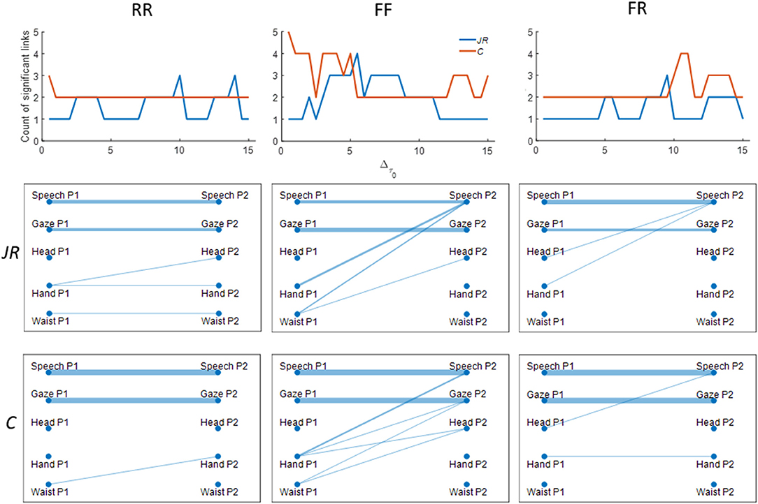
Figure 4. Figures summarizing graph density and topology for interpersonal data calculated using TDSLMAX. Columns correspond to the three levels of hand restraint placed on the interacting pairs. The first row shows the count of significant links as a function of the TDS similarity threshold parameter (Δ_τ0) for both JRQA-based and cross-correlation-based measures. The second and third row are networks showing the significant links between person one (P1) and person 2 (P2) identified by the JRQA-based and cross-correlation-based methods. The thickness of the lines in the graphs indicate the proportion of times that link was identified as significant over all values of Δ_τ0.

FIGURE 5

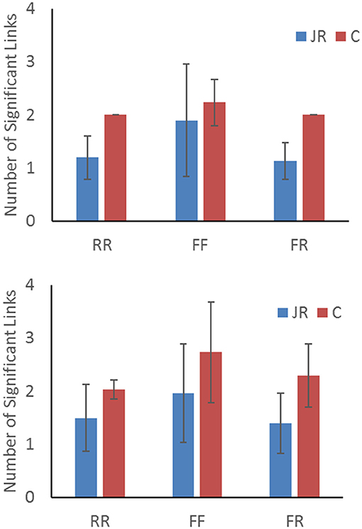
Figure 5. Bar graphs summarizing graph density in terms of number of significant links averaged over all values the TDS similarity threshold parameter(Δ_τ0) for both %TDS (Top) and TDSLMAX (Bottom). Error bars represent ± 1 standard deviation.

On average, the density of the network (i.e., the number of significant links between time series identified by surrogate analyses) was highest in the FF condition regardless of evaluation method. Network densities for RR and FR were very similar, though there is some evidence that coupling in postural dynamics measured at the waist and hand was higher in the RR condition relative to FR, which is consistent with findings using CRQA. Not surprisingly, given the nature of the task, the most reliable interactions between participants were found in their speech and gaze dynamics. Investigations of the network connections showed some differences in the connectivity patterns identified by JRQA and cross-correlation-based statistics, though in aggregate, the patterning in network density as a function of movement constraints were similar between the two approaches. However, JRQA-based statistics appeared to have smaller windows of sensitivity over the Δ_τ0 parameter, while cross-correlation-based approaches were less affected by variations in Δ_τ0. This variation may be a result of JRQA-based statistics being more sensitive to the task constraints relative to cross-correlation-based statistics.

Discussion

In the current project, we showed how TDS can be extended using joint-recurrence quantification analysis (JRQA). We evaluated how TDS metrics obtained with JRQA compare to those obtained with cross-correlation for a variety of multivariate systems, including systems of non-linear oscillators and multivariate behavioral signals measured from dyads performing a joint problem-solving task. Our findings are consistent with previous claims regarding the robustness of the TDS method and show that, despite limitations associated with standard cross-correlation, cross-correlation in the TDS framework offers sensitivity on par with a TDS approach that uses JRQA.

Our findings show that in synthetic systems of non-linear Rössler oscillators with known parameters and outputs, even though JRQA was calculated using all dimensions of a system, cross-correlation provided a qualitatively similar, and perhaps better, ability to detect coupling. Cross-correlation-based approaches were more sensitive to coupling strength when there were larger differences between the systems (e.g., one Rössler system was phase-coherent and one was in the funnel-regime). Though not reported, some of our analyses indicated that output from both the JRQA and cross-correlation methods showed dependence on number of samples and window size in our analyses of the coupled Rössler systems, with slight advantages evident in either approach depending on the parameter selection. However, the general finding that both JRQA and cross-correlation-based approaches to TDS yield largely comparable results, with cross-correlation-based approach showing higher overall sensitivity to interactions between the systems over a range of parameters values, was consistent across our simulations.

For behavioral systems with unknown parameters and unknown dimensionality, we again found similarity in the outputs between JRQA and cross-correlation. Additionally, our current analyses partially contrast with, and perhaps complement, those reported in Tolston et al. [43]. The previous analyses showed that asymmetric restraints on movement resulted in differences in overall postural dynamics relative to conditions of symmetric restraint, while our current analyses indicate a movement restraint placed on either one or both participants in a dyad can result in significantly reduced interpersonal coupling. We remark that Tolston et al. [43] found a similar pattern of higher similarity in RR for head and gaze dynamics, but the general trend was a negative influence of asymmetry in restraint. We believe these differences can be attributed to the fact that CRQA (used in [43]) measures similarity in phase space trajectories and is not sensitive to temporal coupling, whereas TDS measures temporally related stability in coupling. Additionally, the low number of significant links in the interpersonal networks brings to mind the issue laid out by Shockley et al. [48], namely that there is often a large degree of variation in the per subject pair levels of coordination, which can reduce the power of a between-participants analysis. The surrogate method we employed here may be limited in a similar way, though the signals that were most reliably linked, gaze and voice data, are the ones that would reasonably have the strongest levels of interpersonal couplings. The similarity in the findings from the two approaches, combined with some demonstrated instances of higher sensitivity in systems of non-linear oscillators, makes the cross-correlation approach somewhat attractive, in that the JRQA method takes substantially more computational time and researcher effort than the cross-correlation approach, which is faster to compute and has fewer parameters compared to JRQA.

One limitation of the current approach is that it was restricted to the estimation of bivariate dependencies. Importantly, it has been documented that networks constructed via bivariate correlation can result in “transitive closure” [9, 49] in which the indirectly coupled nodes are identified as having a relationship and can result in overly dense networks. Moreover, in order to determine causality, infer directionality of coupling, or rule out spurious relationships in multivariate systems in which strict experimental control is limited or impossible, it will be necessary to extend the current methods to use conditional dependencies that consider the influences other variables [50]. Work has already been conducted to extend the RQA framework in this direction [51, 52] and it would be interesting to combine that approach with the present one, potentially to identify causal networks (e.g., [2]).

In addition, though we did not report individual values, we make note that %TDS and TDSLMAX obtained using JRQA were near ceiling for gaze data, which may be driven by large similarities in gaze fixation time between participants. Further, JRQA and cross-correlation-based approaches were capturing different aspects of gaze coordination; cross-correlation, being based on spatial variation, was sensitive to location fluctuations in the gaze plane, while JRQA was sensitive to mutually recurrent points (i.e., stable gaze fixations). The similarities and potentially complementary differences of the two approaches warrant further investigation.

Finally, it is possible that the expected benefits of using multidimensional data that were not always apparent when using JRQA to compute TDS may be realized by another non-linear method, e.g., average mutual information [53]. Another possibility for future work is that the method may be extended or modified to look at shifted recurrence times (e.g., as in [32]), rather than shifted time series. This approach would be more like a cross-coherence analysis, and some preliminary investigations conducted by the authors showed this method may be sensitive to coupling even when there is a large amount of non-stationary noise added to the system. Further, the current evaluations of coupled oscillators looked only at the effects of feedback coupling, but there are other types of coupling configurations, including linear and non-linear interactions of model terms (i.e., [54]). We also note that, in addition to MAXLINE, other metrics originating in RQA, like mean line length and entropy of line distributions [29], could also be applied to the TDS framework. We leave it to future work to continue to explore the strengths and limitations of these many possibilities.

Data Availability Statement

The datasets for this article are not publicly available. Requests to access the datasets should be directed to Michael Tolston, mtolston@ball.com.

Ethics Statement

The studies involving human participants were reviewed and approved by University of Cincinnati Institutional Review Board. The patients/participants provided their written informed consent to participate in this study.

Author Contributions

MT conducted analyses and contributed to the conceptual development and writing of the manuscript. GF and KS contributed to the conceptual development and writing of the manuscript.

Conflict of Interest

MT was employed by the company Ball Aerospace and Technologies Corporation.

The remaining authors declare that the research was conducted in the absence of any commercial or financial relationships that could be construed as a potential conflict of interest.

Acknowledgments

The authors would like to acknowledge Sara Schneider from the University of California, Merced for her contribution in cleaning the audio data used in this study.

References

1. Bashan A, Bartsch RP, Kantelhardt JW, Havlin S, Ivanov PC. Network physiology reveals relations between network topology and physiological function. Nat Commun. (2012) 3:702–10. doi: 10.1038/ncomms1705

PubMed Abstract | CrossRef Full Text | Google Scholar

2. Runge J, Petoukhov V, Donges JF, Hlinka J, Jajcay N, Vejmelka M, et al. Identifying causal gateways and mediators in complex spatio-temporal systems. Nat Commun. (2015) 6:8502. doi: 10.1038/ncomms9502

PubMed Abstract | CrossRef Full Text | Google Scholar

3. Rheinwalt A, Boers N, Marwan N, Kurths J, Hoffmann P, Gerstengarbe F-W, et al. Non-linear time series analysis of precipitation events using regional climate networks for Germany. Clim Dyn. (2015) 46:1065–74. doi: 10.1007/s00382-015-2632-z

CrossRef Full Text | Google Scholar

4. Runge J, Petoukhov V, Kurths J. Quantifying the strength and delay of climatic interactions: the ambiguities of cross correlation and a novel measure based on graphical models. J Clim. (2014) 27:720–39. doi: 10.1175/JCLI-D-13-00159.1

CrossRef Full Text | Google Scholar

5. Goswami B, Marwan N, Feulner G, Kurths J. How do global temperature drivers influence each other? Eur Phys J Spec Topics. (2013) 222:861–73. doi: 10.1140/epjst/e2013-01889-8

CrossRef Full Text | Google Scholar

6. Ulanowicz RE. Quantitative methods for ecological network analysis. Comput Biol Chem. (2004) 28:321–39. doi: 10.1016/j.compbiolchem.2004.09.001

PubMed Abstract | CrossRef Full Text | Google Scholar

7. Proulx SR, Promislow DE, Phillips PC. Network thinking in ecology and evolution. Trends Ecol Evol. (2005) 20:345–53. doi: 10.1016/j.tree.2005.04.004

PubMed Abstract | CrossRef Full Text | Google Scholar

8. Traud AL, Kelsic ED, Mucha PJ, Porter MA. Comparing community structure to characteristics in online collegiate social networks. SIAM Rev. (2011) 53:526–43. doi: 10.1137/080734315

CrossRef Full Text | Google Scholar

9. Bassett DS, Sporns O. Network neuroscience. Nat Neurosci. (2017) 20:353–64. doi: 10.1038/nn.4502

PubMed Abstract | CrossRef Full Text | Google Scholar

10. Sporns O. Graph theory methods: applications in brain networks. Dialog Clin Neurosci. (2018) 20:111–20.

PubMed Abstract | Google Scholar

11. Diez I, Sepulcre J. Neurogenetic profiles delineate large-scale connectivity dynamics of the human brain. Nat Commun. (2018) 9:3876. doi: 10.1038/s41467-018-06346-3

PubMed Abstract | CrossRef Full Text | Google Scholar

12. Doron KW, Bassett DS, Gazzaniga MS. Dynamic network structure of interhemispheric coordination. Proc Natl Acad Sci USA. (2012) 109:18661–8. doi: 10.1073/pnas.1216402109

PubMed Abstract | CrossRef Full Text | Google Scholar

13. Hui C, Richardson DM. How to invade an ecological network. Trends Ecol Evol. (2018) 34:121–31. doi: 10.1016/j.tree.2018.11.003

PubMed Abstract | CrossRef Full Text | Google Scholar

14. Nie S, Stanley HE, Chen S-M, Wang B-H, Wang X-W. Control energy of complex networks towards distinct mixture states. Sci Rep. (2018) 8:10866. doi: 10.1038/s41598-018-29207-x

PubMed Abstract | CrossRef Full Text | Google Scholar

15. Lü L, Zhang Y-C, Yeung CH, Zhou T. Leaders in social networks, the delicious case. PLoS ONE. (2011) 6:e21202. doi: 10.1371/journal.pone.0021202

PubMed Abstract | CrossRef Full Text | Google Scholar

16. West BJ, Geneston EL, Grigolini P. Maximizing information exchange between complex networks. Phys Rep. (2008) 468:1–99. doi: 10.1016/j.physrep.2008.06.003

CrossRef Full Text | Google Scholar

17. Menck PJ, Heitzig J, Marwan N, Kurths J. How basin stability complements the linear-stability paradigm-Supplemental. Nat Phys. (2013) 9:89–92. doi: 10.1038/nphys2516

CrossRef Full Text | Google Scholar

18. Barahona M, Pecora LM. Synchronization in small-world systems. Phys Rev Lett. (2002) 89:054101. doi: 10.1103/PhysRevLett.89.054101

PubMed Abstract | CrossRef Full Text | Google Scholar

19. Brugere I, Gallagher B, Berger-Wolf TY. Network structure inference, a survey: motivations, methods, and applications. ACM Comput Surv. (2018) 51:24. doi: 10.1145/3154524

CrossRef Full Text | Google Scholar

20. Sporns O, Betzel RF. Modular brain networks. Annu Rev Psychol. (2016) 67:613–40. doi: 10.1146/annurev-psych-122414-033634

PubMed Abstract | CrossRef Full Text | Google Scholar

21. May RM. Thresholds and breakpoints in ecosystems with a multiplicity of stable states. Nature. (1977) 269:471. doi: 10.1038/269471a0

CrossRef Full Text | Google Scholar

22. Scheffer M, Bascompte J, Brock WA, Brovkin V, Carpenter SR, Dakos V, et al. Early-warning signals for critical transitions. Nature. (2009) 461:53–9. doi: 10.1038/nature08227

PubMed Abstract | CrossRef Full Text | Google Scholar

23. Katori Y, Sakamoto K, Saito N, Tanji J, Mushiake H, Aihara K. Representational switching by dynamical reorganization of attractor structure in a network model of the prefrontal cortex. PLoS Comput Biol. (2011) 7:e1002266. doi: 10.1371/journal.pcbi.1002266

PubMed Abstract | CrossRef Full Text | Google Scholar

24. Hesse J, Gross T. Self-organized criticality as a fundamental property of neural systems. Front Syst Neurosci. (2014) 8:166. doi: 10.3389/fnsys.2014.00166

PubMed Abstract | CrossRef Full Text | Google Scholar

25. Ivanov PC, Amaral LAN, Goldberger AL, Havlin S, Rosenblum MG, Struzik ZR, et al. Multifractality in human heartbeat dynamics. Nature. (1999) 399:461–5. doi: 10.1038/20924

PubMed Abstract | CrossRef Full Text | Google Scholar

26. Sameti H, Sheikhzadeh H, Deng L, Brennan RL. HMM-based strategies for enhancement of speech signals embedded in nonstationary noise. IEEE Trans Speech Audio Process. (1998) 6:445–55. doi: 10.1109/89.709670

CrossRef Full Text | Google Scholar

27. Shockley K, Butwill M, Zbilut JP, Webber CL. Cross recurrence quantification of coupled oscillators. Phys Lett A. (2002) 305:59–69. doi: 10.1016/S0375-9601(02)01411-1

CrossRef Full Text | Google Scholar

28. Pikovsky A, Kurths J, Rosenblum M, Kurths J. Synchronization: A Universal Concept in Nonlinear Sciences. New York, NY: Cambridge University Press (2001). doi: 10.1017/CBO9780511755743

CrossRef Full Text | Google Scholar

29. Marwan N, Romano MC, Thiel M, Kurths J. Recurrence plots for the analysis of complex systems. Phys Rep. (2007) 438:237–329. doi: 10.1016/j.physrep.2006.11.001

CrossRef Full Text | Google Scholar

30. Webber C, Zbilut JP. Dynamical assessment of physiological systems and states using recurrence plot strategies. J Appl Physiol. (1994) 76:965–73. doi: 10.1152/jappl.1994.76.2.965

PubMed Abstract | CrossRef Full Text | Google Scholar

31. Romano MC, Thiel M, Kurths J, von Bloh W. Multivariate recurrence plots. Phys Lett A. (2004) 330:214–23. doi: 10.1016/j.physleta.2004.07.066

CrossRef Full Text | Google Scholar

32. Romano M, Thiel M, Kurths J, Kiss I, Hudson J. Detection of synchronization for non-phase-coherent and non-stationary data. Europhys Lett. (2005) 71:466. doi: 10.1209/epl/i2005-10095-1

CrossRef Full Text | Google Scholar

33. Eckmann JP, Kamphorst SO, Ruelle D. Recurrence plots of dynamical systems. Europhys Lett. (1987) 4:973–7. doi: 10.1209/0295-5075/4/9/004

CrossRef Full Text | Google Scholar

34. Schultz AP, Zou Y, Marwan N, Turvey MT. Local minima-based recurrence plots for continuous dynamical systems. Int J Bifurc Chaos. (2011) 21:1065–75. doi: 10.1142/S0218127411029045

CrossRef Full Text | Google Scholar

35. Prado TdL, dos Santos Lima GZ, Lobão-Soares B, do Nascimento GC, Corso G, Fontenele-Araujo J, et al. Optimizing the detection of nonstationary signals by using recurrence analysis. Chaos. (2018) 28:085703. doi: 10.1063/1.5022154

PubMed Abstract | CrossRef Full Text | Google Scholar

36. Kraemer KH, Donner RV, Heitzig J, Marwan N. Recurrence threshold selection for obtaining robust recurrence characteristics in different embedding dimensions. Chaos. (2018) 28:085720. doi: 10.1063/1.5024914

PubMed Abstract | CrossRef Full Text | Google Scholar

37. Marwan N, Kurths J. Cross recurrence plots and their applications. In: Benton CV, editor Mathematical Physics Research at the Cutting Edge. Hauppauge, NY: Nova Science Publishers (2004). p. 101–39.

Google Scholar

38. Zbilut JP, Giuliani A, Webber CL. Detecting deterministic signals in exceptionally noisy environments using cross-recurrence quantification. Phys Lett A. (1998) 246:122–8. doi: 10.1016/S0375-9601(98)00457-5

CrossRef Full Text | Google Scholar

39. Donner RV, Small M, Donges JF, Marwan N, Zou Y, Xiang R, et al. Recurrence-based time series analysis by means of complex network methods. Int J Bifurc Chaos. (2011) 21:1019–46. doi: 10.1142/S0218127411029021

CrossRef Full Text | Google Scholar

40. Xu X, Zhang J, Small M. Superfamily phenomena and motifs of networks induced from time series. Proc Natl Acad Sci USA. (2008) 105:19601–5. doi: 10.1073/pnas.0806082105

PubMed Abstract | CrossRef Full Text | Google Scholar

41. Small M, Zhang J, Xu X. Transforming time series into complex networks. In: International Conference on Complex Sciences. Berlin: Springer (2009). p. 2078–89. doi: 10.1007/978-3-642-02469-6_84

CrossRef Full Text | Google Scholar

42. Theiler J. Spurious dimension from correlation algorithms applied to limited time-series data. Phys Rev A. (1986) 34:2427. doi: 10.1103/PhysRevA.34.2427

PubMed Abstract | CrossRef Full Text | Google Scholar

43. Tolston MT, Shockley K, Riley MA, Richardson MJ. Movement constraints on interpersonal coordination and communication. J Exp Psychol. (2014) 40:1891. doi: 10.1037/a0037473

PubMed Abstract | CrossRef Full Text | Google Scholar

44. Wallot S, Roepstorff A, Mønster D. Multidimensional Recurrence Quantification Analysis (MdRQA) for the analysis of multidimensional time-series: a software implementation in MATLAB and its application to group-level data in joint action. Front Psychol. (2016) 7:1835. doi: 10.3389/fpsyg.2016.01835

PubMed Abstract | CrossRef Full Text | Google Scholar

45. Cao L, Mees A, Judd K. Dynamics from multivariate time series. Phys D. (1998) 121:75–88. doi: 10.1016/S0167-2789(98)00151-1

CrossRef Full Text | Google Scholar

46. Wilcox RR. Introduction to Robust Estimation and Hypothesis Testing. Oxford: Academic Press (2012). doi: 10.1016/C2010-0-67044-1

CrossRef Full Text | Google Scholar

47. Benjamini Y, Hochberg Y. Controlling the false discovery rate: a practical and powerful approach to multiple testing. J R Stat Soc Series B. (1995) 57:289–300. doi: 10.1111/j.2517-6161.1995.tb02031.x

CrossRef Full Text | Google Scholar

48. Shockley K, Baker AA, Richardson MJ, Fowler CA. Articulatory constraints on interpersonal postural coordination. J Exp Psychol. (2007) 33:201–8. doi: 10.1037/0096-1523.33.1.201

PubMed Abstract | CrossRef Full Text | Google Scholar

49. Zalesky A, Fornito A, Bullmore E. On the use of correlation as a measure of network connectivity. Neuroimage. (2012) 60:2096–106. doi: 10.1016/j.neuroimage.2012.02.001

PubMed Abstract | CrossRef Full Text | Google Scholar

50. Kralemann B, Pikovsky A, Rosenblum M. Reconstructing effective phase connectivity of oscillator networks from observations. New J Phys. (2014) 16:085013. doi: 10.1088/1367-2630/16/8/085013

CrossRef Full Text | Google Scholar

51. Builes-Jaramillo A, Ramos AM, Poveda G. Atmosphere-land bridge between the Pacific and tropical North Atlantic SST's through the Amazon River basin during the 2005 and 2010 droughts. Chaos. (2018) 28:085705. doi: 10.1063/1.5020502

PubMed Abstract | CrossRef Full Text | Google Scholar

52. Ramos AM, Builes-Jaramillo A, Poveda G, Goswami B, Macau EE, Kurths J, et al. Recurrence measure of conditional dependence and applications. Phys Rev E. (2017) 95:052206. doi: 10.1103/PhysRevE.95.052206

PubMed Abstract | CrossRef Full Text | Google Scholar

53. Prichard D, Theiler J. Generalized redundancies for time series analysis. Phys D. (1995) 84:476–93. doi: 10.1016/0167-2789(95)00041-2

CrossRef Full Text | Google Scholar

54. Ma H-C, Chen C-C, Chen B-W. Dynamics and transitions of the coupled Lorenz system. Phys Rev E. (1997) 56:1550. doi: 10.1103/PhysRevE.56.1550

CrossRef Full Text | Google Scholar

Appendix A: Audio Data Pre-processing

Audio data were collected using Motorola H15 Bluetooth Headsets worn by each participant. Because both participants were in the same room when they were being recorded, each participant's audio data were at least somewhat contaminated with the voice of their partner. To address this issue, audio data were pre-processed using the noise reduction feature of the audio program Audacity. To do so, the data were imported into Audacity and a portion of the waveform was selected where only the partner of the participant whose data was being analyzed was heard to be speaking clearly for several seconds. Next, a profile for this contamination was obtained, and the reduction was applied to the full waveform with the following parameters: noise reduction (dB) was set to 50, sensitivity was set to 25, and frequency smoothing was set to 3. Following this noise reduction, waveform data were aggregated by summation of the squared amplitudes to a 30 Hz sample rate. These data were then smoothed using a moving mean filter with a window size equal to 15 samples (2 Hz). These data were then standardized to have values between 0 and 1 and were converted to a binary sequence indicating whether the participant was talking by thresholding the amplitude time series. Finally, a moving mode filter with a window size equal to 15 samples was applied to the thresholded data. This process was repeated for a range of thresholds for both participants and the set of values that resulted in the largest negative cross-correlation between the two binary signals were chosen for each pair of signals.