A New Bayesian Methodology for Nonlinear Model Calibration in Computational Systems Biology

1. Introduction

In recent years omics technologies have tremendously advanced allowing the identification and quantification of molecules at the DNA, RNA and protein level [1, 2]. These high-throughput experiments produce huge amounts of data which need to be managed and analyzed in order to extract useful information [3]. In this context, mathematical models play an important role since they process these data and simulate complex biological phenomena. The main purpose of mathematical modeling is to study cellular and extracellular biological processes from a quantitative point of view and highlight the dynamics of cellular components interactions [4]. Moreover, models represent an excellent tool to predict the value of biological parameters that may not be directly accessible through biological experiments because they would be time consuming, expensive or not feasible [5]. One of the most common modeling techniques consists in representing a biological event, such as a signaling pathway, through a system of Ordinary Differential Equations (ODEs), which describes the dynamic behavior of state variables, i.e., the variation of species concentration in the system as a function of time [6]. Currently, the most used kinetic laws in ODE models can be divided into three types: the law of mass action, the Michaelis-Menten kinetic and the Hill function [7, 8]. However, these equations contain unknown parameters which have to be estimated in order to properly simulate the model and represent the problem under study. Typically, the calibration process of a model consists in the inference of parameters in order to make output variables as close as possible to the experimental dataset [9]. Hence, a calibrated model can be used to predict the time evolution of substances for which enough information or measures are not available. The most common methodologies for parameter estimation can be divided in two classes: the frequentist and the Bayesian approach [5, 10]. Frequentist methods aim at maximizing the likelihood function f(y|p), which is the probability density of observing the dataset y given parameter values p [11]. Under the hypothesis of independent additive Gaussian noise with constant and known variance for each measurement, the Maximum Likelihood Estimation (MLE) problem is equivalent to the minimization of an objective function, which compares simulated and experimental data [12, 13]. Common objective functions are the sum of squared residuals or the negative log-likelihood [14]. When the variances of measurement noise are not known, they are included in the likelihood as additional terms to estimate [13]. Different optimization algorithms are then employed to estimate the best parameter values. They implement global and/or local techniques and return in output the best fit between simulated and real data.

Since these optimization methods return only one solution for the parameter vector, i.e., the best fit, then parameter estimation is usually combined with identifiability analysis, in order to assess how much uncertainty there is in the parameter estimate [15]. Identifiability analysis is typically performed through the computation of confidence intervals for all estimated parameters. A confidence interval is the range where the true parameter value is located with a certain frequency. In this context, Profile Likelihood (PL) is a widely used data-based algorithm for structural and practical identifiability analysis [16].

On the other hand, the Bayesian approach considers parameters as random variables, whose joint posterior distribution f_P|y(p) is estimated through the Bayes theorem: $f_{\text{P}|\text{y}}(\text{p})=\frac{f(\text{y}|\text{p})f_{\text{P}}(\text{p})}{f(\text{y})}$, where f(y) is the marginal density for y and f_P(p) is the prior probability density of parameters [17]. Through f_P(p) it is possible to include a priori beliefs about parameter values [18]. The joint posterior density automatically provides an indication of the uncertainty of the parameter inference and gives major insights about the robustness of the solution [19]. Since computing the posterior distribution analytically is usually not feasible, sampling based techniques are used to estimate it [12, 17]. Two classes of sampling methods widely used are the Markov chain Monte Carlo (MCMC) and the Approximate Bayesian Computation Sequential Monte Carlo (ABC-SMC) [12]. MCMC algorithms approximate the posterior distribution with a Markov chain, whose states are samples from the parameter space. Their major advantage is the ability to infer the posterior distribution which is known only up to a normalizing constant [20]. The ABC-SMC algorithms evaluate an approximation of the posterior distribution through a series of intermediate distributions, obtained by iteratively perturbing the parameter space. Each iteration selects only those parameters that give rise to a distance function under a predefined threshold [21].

In this paper, our main purpose is to introduce a new version of the standard ABC-SMC approach, called Conditional Robust Calibration (CRC), for parameter estimation of mathematical models.

As in all ABC-SMC methods, CRC is an iterative procedure based on the parameter space sampling and on the estimation of the probability density function (pdf) for each model parameter. However, it presents different aspects that differentiate it from the other existent methodologies. The distinctive features of CRC are: (i) a major control of the computational costs of the procedure, (ii) the definition of multiple objective functions, one for each output variable, (iii) the conditional robustness analysis (CRA) [22], in order to determine the influence of each model parameter on the observables.

We validate this new methodology on different ODE models of increasing complexity. Here we present the results of CRC applied to three models, two with in silico noisy data and one with experimental proteomic data. We also calibrate all the models using the PL approach, through the software Data2Dynamics (D2D) [23] and the standard ABC-SMC, through the ABC-SysBio software [19].

Moreover, in order to provide a reliable and complete comparison with the state of the art of this field, we also apply the Delayed Rejection Adaptive Metropolis (DRAM) algorithm through the MCMC toolbox [24, 25] to all the models presented in the Results section. DRAM combines two well-known strategies that are common in the MCMC schemes: adaptive Metropolis samplers and delayed rejection [24]. However, DRAM is not the only algorithm that improves the standard MCMC sampler. As shown in [26], many other similar and efficient methodologies are very popular in the literature. Since the underlying concept of these methodologies is the sampling from a proposal distribution, the common objective of this class of methods is to speed-up and improve the performance of the MCMC sampler. Some examples are the Multiple Try Metropolis (MTM) algorithm [27] and the Adaptive Gaussian Mixture Metropolis-Hastings [28, 29].

Our results show that CRC is successful in all examples and that its innovation features are critical when calibrating models with an high number of parameters and output variables. Especially when compared to ABC-SMC, CRC does not remain stuck in intermediate iterations because of its reduced computational cost and it is able to estimate parameter values of a model with an higher accuracy due to the definition of objective functions specific for each output variable. Finally, it also introduces the concept of conditional robustness that is different from standard identifiability.

2. Materials and Methods

2.1. ODE Model

Consider a deterministic ordinary nonlinear dynamical system:

$\begin{array}{l}\stackrel{.}{\text{x}}(t)=f(\text{x}(t),\text{u}(t),\theta ),\text{x}(0)=x_0,\text{x}\in {ℝ}^n,\theta \in \Theta \\ \text{y}(t)=h(\text{x}(t),\text{u}(t),\gamma ),\text{y}\in {ℝ}^m,\gamma \in {ℝ}^s,\text{u}\in {ℝ}^g\end{array}$

where x is the state space vector, u denotes the external input vector, and y denotes the output responses of the system, i.e., the observables, which are usually derived from experimentally observed data. The vector θ denotes the dynamical system parameters, taking values in the parameter space Θ, a subset of the positive orthant ${ℝ}_{>0}^q$. The vector function f is indeed defined over the following sets: f(·): ℝⁿ × ℝ^g × ℝ^q → ℝⁿ. The observation function h(·): ℝⁿ × ℝ^g × ℝ^s → ℝ^m maps the state variables to the vector of observable quantities y. Usually, not all states of the system can be directly measured, so that it is common to have m < n. Vector γ contains scaling and offset parameters when measurements of the observables are performed. Setting p = {θ, γ, x(0)}, p ∈ ℝ^q+s+n, the model is completely determined. We assume that the parameter vector p is constant over time. We assume that data are collected at discrete time points t_j ∈ [t₀, t_k] and thus the generic data measure can be written as:

$\begin{array}{ll}{y}_{ij}^{*}=y_{ij}+{\tau }_{ij},i=1,\dots ,m& (1)\end{array}$

where y_ij is the measurement and τ_ij is the unknown measurement error.

2.2. General Theory

The parameter vector of a mathematical model can be considered as a random variable P: ℙ → ℝ^(q+s+n), where ℙ is the set of all possible vectors in the parameter space and ℝ^(q+s+n) is the measurable space. Thus, a given vector p in the parameter space is one of the possible realizations of P. Let f_P(p) denote the prior distribution. Our goal is to approximate the target posterior distribution, f_P|y(p) ∝ f(y|p)f_P(p), where f(y|p) is the likelihood density that describes the model. This is the pdf of the output variables of the model when parameters are distributed according to the prior f_P(p). To this purpose, we develop CRC, a variant of the ABC-SMC iterative algorithm. As it is well-established in this class of techniques, at the beginning of each iteration z, CRC samples parameters from a proposal distribution q^z(p). However, differently to standard ABC approaches, we generate a fixed number N_S of samples from q^z(p) along the different iterations. Then the fitting between observed and simulated data is measured through the computation of a distance function. CRC defines, at each iteration, multiple distance functions d_i,p, each one associated with a single component of the output function, without the employment of any summary statistic. The distance functions defined above are the objective functions that CRC reduces iteration by iteration until a convergence criterion is met. Since parameter vector P is a random variable, d_i,p can be considered a realization of the random variable D_i that describes the distribution of the distance function, corresponding to the i-th output. The random variable D_i models the distribution of the error between simulated and real data when the parameter are sampled. Accordingly, at each iteration we define a set of thresholds ${ϵ}_i^z$ that specify the maximum accepted level of agreement between each observable and the corresponding simulated data. At each iteration we obtain different parameter sets $P_{S,{ϵ}_i^z}$. Each set contains only those parameters that yield the values of a specific distance function under the corresponding threshold. Then, all these sets are intersected in order to obtain a single parameter set, $P_{S,{ϵ}^z}$, that ensures the compliance with all the thresholds. $P_{S,{ϵ}^z}$ contains samples of the approximate posterior distribution $f_{\text{P}|P_{S,{ϵ}^z}}(\text{p})$. As for other ABC methods, if at the end of the z-th iteration a predefined stopping criterion is not satisfied, another iteration of CRC is performed, sampling from a new proposal distribution. Since the region of interest of the approximate posterior distribution is the one with highest probability, the proposal for the next iteration, q^z+1(p), is centered on the mode of $f_{\text{P}|P_{S,{ϵ}^z}}(\text{p})$. In order to increase the frequency of N_S samples in this region, the boundaries of q^z+1(p) are tighter than those of q^z(p). The algorithm terminates when the thresholds are sufficiently small. The output of CRC is $f_{\text{P}|P_{S,{ϵ}^{\zeta }}}(\text{p})$ where ζ is the number of the last iteration and its mode ${\text{p}}_m^{\zeta }$ is the vector that reproduces the observed data with the highest probability.

2.3. CRC Algorithm

Figure 1 sums up the main steps of the CRC algorithm.

1. Sampling the parameter space and the posterior distribution. Generate a predefined number of samples N_S from the proposal distribution q^z(p). If z = 1 the proposal distribution is the prior f_P(p). Let P_S be the set of parameter samples generated from q^z(p). For each sample p ∈ P_S, simulate the model in order to compute a dataset y = [y_i(t_j)],  i = 1, …, m and j = 0, …, k. This dataset contains the samples of the likelihood function.

2. Computation of the distance functions and pdf estimation. For each p ∈ P_S, as many distance functions as observables are computed, i.e., $d_{i,\text{p}}(y_i,y_i^{*})$, ∀i = 1, …, m, where $y_i^{*}$ is the i-th variable of the experimental dataset and y_i is the sequence of simulated values over time for that variable. Then the associated densities are estimated using a kernel density approach. Let denote with f_Di(d_i,p) the pdf of D_i, where D_i is a transformation from the random variable P and whose realizations are given by d_i,p.

3. Parameter sets identification. For each distance function we define a threshold ${ϵ}_i^z\ge 0$ which is the quartile of level α of f_Di(d_i,p) and we obtain the following subset:

$\begin{array}{ll}T({ϵ}_i^z,d_{i,\text{p}})=\{d_{i,\text{p}}\le {ϵ}_i^z:{\displaystyle {\int }_0^{{ϵ}_i^z}}{f}_{D_i}(d_{i,\text{p}})\text{d}{d}_i=\alpha \}.& (2)\end{array}$

Therefore $T({ϵ}_i^z,d_{i,\text{p}})$ induces the subset $P_{S,{ϵ}_i^z}\in P_S$ defined as:

$\begin{array}{ll}{P}_{S,{ϵ}_i^z}=\left\{p\in P_S:d_{i,\text{p}}\in T({ϵ}_i^z,d_{i,\text{p}})\right\}.& (3)\end{array}$

4. Intersection of Parameter Sets. Let denote ${ϵ}^z=\left\{{ϵ}_1^z,{ϵ}_2^z,\dots ,{ϵ}_i^z,\dots ,{ϵ}_m^z\right\}$ the set of thresholds corresponding to each observable at iteration z. We select the parameter samples that satisfy the conditions specified in the previous step simultaneously for all observables. This implies the definition of the following subset of P_S:

$\begin{array}{ll}{P}_{S,{ϵ}^z}=\{{\displaystyle \bigcap _{i=1}^m}{P}_{S,{ϵ}_i^z}\}.& (4)\end{array}$

Thus, in the parameter space, the accepted samples belong to the approximate posterior distribution $f_{\text{P}|P_{S,{ϵ}^z}}(\text{p})$. Figure 1B clarifies the meaning of Equation (4): conceptually, in this step we identify and intersect the low tails of m distance function distributions, f_Di(d_i,p), in order to obtain, in the parameter space, the joint conditional density $f_{\text{P}|P_{S,{ϵ}^z}}(\text{p})$. If the values of thresholds in ϵ^z satisfy the stopping criterion, the algorithm terminates and the output is $f_{\text{P}|P_{S,{ϵ}^z}}(\text{p})$. Otherwise go to step 6.

5. Update the proposal distribution. From $f_{\text{P}|P_{S,{ϵ}^z}}(\text{p})$ we select the mode vector ${\text{p}}_m^z$. The proposal distribution of the subsequent iteration, q^z+1(p), is defined as:

$\begin{array}{ll}{q}^{z+1}(\text{p}):=q^z(\text{p};{\text{p}}_m^z,U^{z+1},L^{z+1}),& (5)\end{array}$

where $q^z(\text{p};{\text{p}}_m^z,U^{z+1},L^{z+1})$ is the proposal distribution at the current iteration z.

FIGURE 1

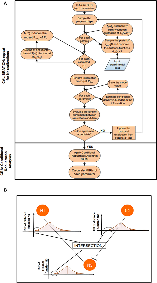
Figure 1. CRC algorithm. (A) The flowchart of CRC is divided in two main phases: model calibration and robustness analysis. (B) Detail of steps 3–5 of CRC. N1, N2, and N3 represent three model observables that interact among each other. For each observable, a distance function d_i,p is computed and the corresponding pdf f_Di(d_i,p) is estimated. We are interested only in the low tail of each pdf, since it is the region where the model observables are closer to the experimental data. Then, all the low tails are intersected among each other to identify $P_{S,{ϵ}^z}$.

Note that while the shape of the proposal distribution does not change over the different iterations, the mean value and the upper and lower boundaries of the proposal do. The mean value is updated according to the mode ${\text{p}}_m^z$ and the upper and lower boundaries, respectively U^z+1 and L^z+1, are shrunk through the following formula:

$\begin{array}{lll}{U}^{z+1}=\frac{U^z+k_{U,1}}{k_{U,2}},& L^{z+1}=\frac{L^z+k_{L,1}}{k_{L,2}}& (6)\end{array}$

where k_{U, 1}, k_{U, 2}, k_L,1, and k_L,2 are constants set by the user. They regulate the percentage variation of the lower and upper boundaries from the mode ${\text{p}}_m^z$. Once the new proposal distribution is defined, restart from step 1.

In Table 1, the pseudocode associated to each step of the algorithm is presented. In the next section there is a detailed explanation of how the different tuning parameters have to be properly set.

TABLE 1

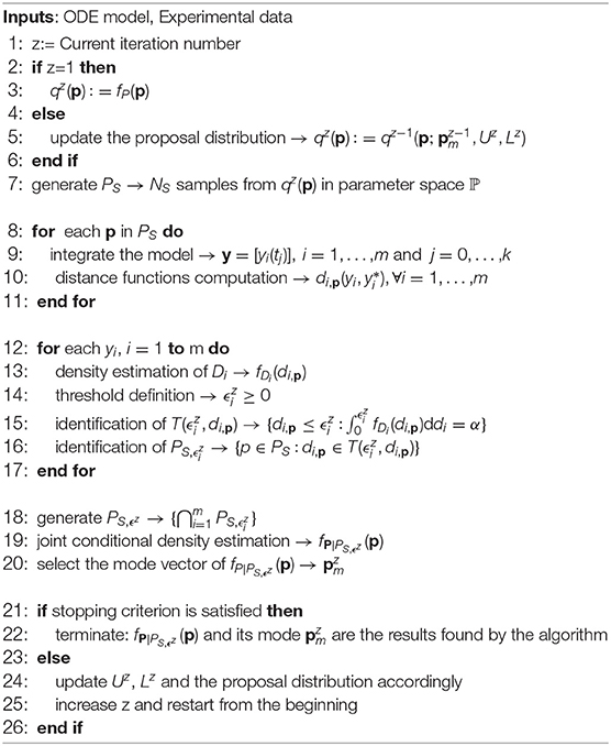
Table 1. CRC algorithm: pseudocode of a generic iteration z of the algorithm.

2.3.1. Tuning Parameters

In this section, we discuss the setting of the tuning parameters of the proposed algorithm. First of all, it is necessary to choose a sampling technique for the parameter space. The objective is to generate a fixed number N_S of samples that optimally cover the entire parameter space defined by the proposal distribution. To this purpose, we use Latin Hypercube Sampling (LHS) because it divides the multidimensional parameter space in $N_S^{|\text{p}|}$ regions and guarantees that each region is represented by a single sample [30, 31]. Since several studies indicate that log-transforming the parameters usually yields a better performance, we use as sampling schema the Logarithmic Latin Hypercube Sampling (LoLHS) [32]. A comparison of the results of CRC using LHS and LoLHS can be found in [33]. As for the number of samples N_S, it is fixed in advance taking into account the dimension of the parameter space and the number of observables of the model.

Then, at each iteration the choice of the threshold values strictly depends on two constraints. First of all, in order to approximate the posterior distribution, tolerances have to be set so that ${ϵ}_i^z\le {ϵ}_i^{z-1}$. According to [22, 34], to generate a reliable non-parametric estimation of the conditional density, at least 1,000 samples of $P_{S,{ϵ}^z}$ are necessary. Thus, tolerances ${ϵ}_i^z$ are chosen in order to ensure that the cardinality of $P_{S,{ϵ}^z}$ is at least 1,000.

Moreover, different combinations of tolerances may lead to the fulfillment of this condition. Therefore, as a guideline, threshold values can be chosen so that the number of accepted samples for each distance function $d_{i,\text{p}}(y_i,y_i^{*})$ is similar as much as possible for all output variables. As the number of iteration increases, thresholds progressively shift toward zero and, as in the standard ABC-SMC method [35], this guarantees that the approximate posterior distribution $f_{\text{P}|P_{S,{ϵ}^z}}(\text{p})$ evolves toward the desired posterior distribution f_P|y(p).

The constraints explained above regarding the choice of the thresholds are also influenced by N_S. For a given set of thresholds ϵ^z, the higher the value of N_S the higher is the cardinality of $P_{S,{ϵ}^z}$. Thus, increasing N_S, it is more likely to reach lower threshold values that satisfy $|P_{S,{ϵ}^z}|>1,000$. However, N_S has also great impact on the computational cost of CRC and, for these reasons, its choice is a trade-off between the accuracy of the posterior estimation and the efficiency of CRC.

Another tuning parameter of CRC is the definition of the distance function that is used to measure the level of agreement between simulations and experimental data.

Here, we propose two different distance functions that can be used as objective functions when running CRC. The first one, called Absolute Distance Function (ADF), is the l-norm sum, over the whole time points set, of the distance between simulated and real data. Equation (7) formalizes it:

$\begin{array}{ll}AD{F}_i={\displaystyle \sum _{j=1}^k}\Vert y_i(t_j)-y_{ij}^{*}{\Vert }_{l}i=1,\dots ,m.& (7)\end{array}$

As an alternative, Equation (8) normalizes the error between simulated and real data with the corresponding point in the dataset. Moreover, the summation is divided by the number of available time points, thus Equation (8) represents the mean percentage error on each time point.

$\begin{array}{ll}AND{F}_i=\frac{1}{k}{\displaystyle \sum _{j=1}^k}\frac{\Vert y_i(t_j)-y_{ij}^{*}{\Vert }_l}{y_{ij}^{*}}i=1,\dots ,m.& (8)\end{array}$

In this paper we set l = 1, thus we use an l₁ norm, because it is robust to measurement noise, i.e., outlier-corrupted data [36]. The criterion that guides the user in the choice of the best distance function regards the range of variation of the available data. For a given absolute error (Equation 7), the corresponding percentage error (Equation 8) produces a bias. Thus, Equation (8) is preferred when the model and data are normalized.

Finally, as explained above, parameters k_U,1, k_U,2, k_L,1, and k_L,2 in Equation (6) determine the percentage shrinkage of the lower and upper boundaries of the proposal distribution. Iteration by iteration the percentage distance of the lower and upper boundaries of f_P(p) from the mode value is reduced.

In CRC the number of necessary iterations is not known a priori because the algorithm terminates when the stopping criterion is satisfied.

2.4. Conditional Robustness Analysis

The goal of the second phase of CRC is to perform a conditional robustness analysis (CRA) in order to identify which parameters mostly influence the output variables behavior [22]. To this purpose, we apply the conditional robustness algorithm in [22, 37]. Starting from ${\text{p}}_m^{\zeta }$, i.e., the mode in the parameter space obtained in the last CRC iteration, we sample the parameter space using LHS and choosing as evaluation functions the distance functions d_i,p ∀i = 1, …, m previously defined during the calibration process. For each distance function, we define two thresholds ${\eta }_i^L\ge 0$ and ${\eta }_i^U\ge 0$ which are the quartiles of level β and λ respectively, obtaining the following subsets:

$\begin{array}{ll}T({\eta }_i^L,d_{i,\text{p}})=\{d_{i,\text{p}}\le {\eta }_i^L:{\displaystyle {\int }_0^{{\eta }_i^L}}{f}_{D_i}(d_{i,\text{p}})\text{d}{d}_i=\beta \},& (9)\end{array}$

$\begin{array}{ll}T({\eta }_i^U,d_{i,\text{p}})=\{d_{i,\text{p}}\ge {\eta }_i^U:{\displaystyle {\int }_{{\eta }_i^U}^{+\infty }}{f}_{D_i}(d_{i,\text{p}})\text{d}{d}_i=\lambda \}.& (10)\end{array}$

Thus, $T({\eta }_i^L,d_{i,\text{p}})$ and $T({\eta }_i^U,d_{i,\text{p}})$ contain values of the distance functions d_i,p that are, respectively smaller and larger than the defined thresholds ${\eta }_i^L$ and ${\eta }_i^U$. Therefore, $T({\eta }_i^L,d_{i,\text{p}})$ and $T({\eta }_i^U,d_{i,\text{p}})$ induce two subsets in the parameter space P_S:

$\begin{array}{ll}{P}_{S,{\eta }_i^L}=\{p\in P_S:d_{i,p}\in T({\eta }_i^L,d_{i,p}))\},& (11)\end{array}$

$\begin{array}{ll}{P}_{S,{\eta }_i^U}=\{p\in P_S:d_{i,\text{p}}\in T({\eta }_i^U,d_{i,\text{p}})\}.& (12)\end{array}$

The resulting conditioning sets are:

$\begin{array}{ll}{P}_{S,{\eta }^L}=\{{\displaystyle \bigcap _{i=1}^m}{P}_{S,{\eta }_i^L}\},P_{S,{\eta }^U}=\{{\displaystyle \bigcap _{i=1}^m}{P}_{S,{\eta }_i^U}\}.& (13)\end{array}$

$P_{S,{\eta }^L}$ and $P_{S,{\eta }^U}$ define two regions in the parameter space, whose samples belong to the distributions $f_{\text{P}|P_{S,{\eta }^L}}(\text{p})$ and $f_{\text{P}|P_{S,{\eta }^U}}(\text{p})$.

The two conditional densities are employed in the calculation of the Moment Independent Robustness Indicator (MIRI) [22, 34] according to the following formula:

$\begin{array}{ll}\mu ={\displaystyle \int }|f_{\text{P}|P_{S,{\eta }^L}}(\text{p})-f_{\text{P}|P_{S,{\eta }^U}}(\text{p})|\text{d}\text{p}.& (14)\end{array}$

Vector μ contains MIRI values of all the components of parameter vector p. Due to its definition, the MIRI value of each parameter is included in the interval [0, 2]. MIRIs measure the level of intersection between the two pdfs included in the calculus: the higher the resulting value and the more well separated are the conditional densities. Parameters with higher values of the MIRI have a major impact on output variables because there is a larger shift between the two conditional densities used for MIRI calculation. This means that different ranges of values for parameters with an high MIRI value lead the model observables to completely different behaviors. On the other hand, parameters with a low MIRI value do not affect the observables because their conditional densities overlap.

2.5. Benchmarking Algorithms

In this section, we give a brief overview of three methods against which CRC is compared: Approximate Bayesian Computation Sequential Monte Carlo (ABC-SMC), Profile Likelihood (PL), and Delayed Rejection Adaptive Metropolis (DRAM).

2.5.1. ABC-SMC

Since the CRC algorithm is a novel version of the standard ABC-SMC, in the current section we keep the mathematical notation consistent for those variables that have the same meaning.

ABC methods are a set of Bayesian methods for parameter estimation and model selection. They can be used to evaluate posterior distributions without having to calculate likelihoods. These methods are based on a comparison between observed and simulated data and thus are particularly useful when the likelihood function is too costly to evaluate [35]. ABC approaches usually proceed by: (i) sample a parameter vector p from a proposal distribution q(p); (ii) simulate a dataset y(t) from the model having parameters p; (iii) calculate a summary statistic s of the observables y of the model; (iv) calculate a distance function d_p(s,s^*) between simulated and experimental data and accept p only if $d_{\text{p}}(\text{s},{\text{s}}^{*})\le ϵ$ where ϵ is the tolerance level. Usually the distance function is defined on the full dataset. The simplest ABC algorithm is the ABC rejection sampler that implements the points described above in a single iteration, thus sampling the parameters only from the prior f_P(p) [38]. An improvement of the first version of ABC algorithm is ABC based on Markov chain Monte Carlo (ABC-MCMC algorithm), that exploits a Markov chain to explore the parameter space [39]. Conversely, ABC-SMC is a particular class of ABC algorithms based on SMC sampling, which seeks to uncover an approximation of the true posterior distribution in a sequential manner through a series of intermediate distributions. It proceeds with the following steps:

• define a tolerance schedule ϵ¹ > ϵ² > …ϵ^T ≥ 0;

• at the first iteration, sample parameter values, called particles, from a prior distribution, until N particles are obtained for which the distance is smaller than ϵ¹; for each particle is then computed a weight;

• for the further iterations, a particle is sampled from the previous population and perturbed with a perturbation kernel, until N accepted particles are selected. Weights are calculated for all accepted particles;

• the same procedure described above is repeated until N particles are selected in the last population.

The last population is the approximation of the posterior distribution f_P|y(p). The ABC-SMC method is fully implemented in the ABC-SysBio software, a Python package for parameter estimation and model selection in the ABC framework [19]. A variant of the standard ABC-SMC algorithm is its population-based version, ABC-PMC [21]. The main feature of ABC-PMC algorithms is the adaptive calculation of the distance function and of the threshold at each iteration, based on the previous iteration's simulations.

2.5.2. Comparison Between ABC-SMC and CRC

Since CRC is a novel version of ABC-SMC, in this section we highlight the main differences between the two algorithms.

First of all, in the ABC-SMC algorithm, both the number of iterations and the threshold schedule have to be chosen in advance before running the whole procedure. Moreover, the total number of samples generated at each iteration is not known. The framework of the algorithm requires to specify the number of parameter samples, N, whose corresponding distance functions are below the threshold of the current iteration. Thus, for each iteration it is not known how many times the model will be integrated and, as the threshold is decreased, more samples are required to meet the constraint. The combination of these two aspects of the algorithm does not guarantee that the desired level of agreement between experimental and simulated data will be reached in a reasonable amount of time. In CRC, on the other hand, the approach is overturned. The number of samples N_S, that are generated at each iteration, is fixed and, on the contrary, the thresholds are not fixed in advance but they are chosen dynamically iteration by iteration. This guarantees that the time to perform each iteration is limited and at the end of each iteration a user defined stopping criterion is evaluated in order to decide whether or not to start again from the beginning.

Another relevant difference between the two algorithms is that CRC defines a distance function for each output variable without the employment of any summary statistic. ABC-SMC, on the contrary, defines a unique distance function regardless of the number of output variables of a model and it is often used with summary statistics. The effect of defining a single distance function has a great impact in the accuracy of model calibration especially when the model has an high number of parameters and/or output variables.

Finally, in the ABC-SMC framework, once a particle is sampled from a population it is perturbed with a kernel before simulating the model and if that particle is accepted a corresponding weight is computed (mathematical details are in [35]). As a consequence, in ABC-SMC, the way each population is updated iteration by iteration strictly depends on the kernel, that also influences the speed of convergence. In CRC, on the other hand, it is not used any perturbational kernel and at the end of each iteration, once the set $P_{S,{ϵ}^z}$ is identified, the empirical conditional density $f_{\text{P}|P_{S,{ϵ}^z}}(\text{p})$ is estimated. The proposal distribution of the next iteration is updated using the mode of the distribution cited above and, through Equation (6), the percentage of variation from the mode of each parameter is shrunk.

2.5.3. Profile Likelihood (PL)

PL is a framework for parameter estimation and uncertainty analysis that belongs to the frequentist class. As in the Bayesian approach, the starting point is the likelihood function that needs to be estimated. Assuming independent additive Gaussian noise with constant variance, maximizing the likelihood means minimizing the Residual Sum of Squares (RSS), commonly denoted as χ²(p) where p is the estimated parameter vector. An optimization algorithm is commonly used to perform estimation. It can be deterministic, stochastic or hybrid [12]. In the class of stochastic algorithms, examples of commonly used methods are the so-called Genetic Algorithms (GA) and Simulated Annealing (SA). GA are iterative searching methods based on a natural selection process that mimics biological evolution. Starting from an initial population, at each iteration, a new population is generated until it evolves toward the optimal solution [40]. SA mimics the process of heating a material and then slowly lowering the temperature. It is a particular application of the Metropolis-Hastings algorithm. At each iteration a new point is generated and accepted according to an acceptance function, based on the temperature parameter [41]. Among deterministic algorithms, nonlinear least-squares (lsqnonlin) is considered one of the fastest and most reliable for common problems in Systems Biology [11, 13]. LHS can be used for setting initial parameters in a multi-start approach in order to avoid local optima as much as possible. For a performance analysis of optimization procedures see [11]. Once an optimal parameter set is obtained, it is important to assess the influence of all parameters on model behavior. The confidence interval $\left[{\sigma }_i^{-},{\sigma }_i^{+}\right]$ of a parameter is a measure of its identifiability. It means that the true value of a parameter is located within this interval with a given probability α. To compute confidence intervals, PL is one the most employed algorithms. It is based on the following formula:

$\begin{array}{ll}{\chi }_{PL}^2(p_i)=mi{n}_{j\ne i}\left[{\chi }^2(\text{p})\right],& (15)\end{array}$

which means that, for each parameter p_i, the function χ² is reoptimized with respect to all parameters p_j≠i. The process starts from the best fit and stops when the fit becomes unacceptable or a certain stopping criterion is met. At the end of it, a profile for each parameter is obtained. A parameter is declared structural non-identifiable if it has a flat profile, while it is practical non-identifiable if it has a minimum but the profile flattens out in one of the directions of χ² (increasing or decreasing direction of p_i). In all the other cases, a parameter is considered identifiable [14].

The PL methodology works by transforming the parameter space from linear to logarithmic. Moreover, it has different tuning parameters that can be set by the user. It is possible to choose the lower and upper bounds for the parameters, the maximum number of steps along the profile for each parameter as well as the maximum and minimum step size. Moreover, in the likelihood function, the measurement noise is modeled as normal or log-normal distribution and it can be fitted simultaneously to the dynamical model.

2.5.4. DRAM

DRAM algorithm is an improved and modified version of the standard Metropolis-Hastings (MH) algorithm [24]. This algorithm belongs to the Markov Chain Monte Carlo (MCMC) methods, which approximate the posterior distribution of the parameter vector through a Markov chain [42]. One of the advantages of such methods is the possibility of sampling from an arbitrary pdf known up to a normalizing constant. DRAM is a strategy to combine the Delayed Rejection (DR) and Adaptive Metropolis (AM) estimators. When a candidate parameter sample is rejected, DRAM finds a new point exploiting also the information about the rejected one. In DR, given p_n as the current position of the chain, the first proposal move, h_n,1 is performed as in MH and thus it is accepted with probability:

$\begin{array}{ll}{\alpha }_{n,1}(p_n,h_{n,1})=min(1,\frac{f(h_{n,1}|\text{y})q_{n,1}(h_{n,1},p_n)}{f(p_n|\text{y})q_{n,1}(p_n,h_{n,1})}),& (16)\end{array}$

where q_n,1(·) is the proposal distribution. The probability distribution f(h_n,1|y) is computed as f(h_n,1|y) = f(y|h_n,1)π(h_n,1), where f(y|h_n,1) is the likelihood and π(h_n,1) is the prior function. In case of rejection of the proposed sample, the second move depends both on the current state of the chain and on the rejected sample. This expedient gives the name “Delayed” to the DR algorithm. The delayed mechanism can be iterated and interrupted at any stage. The mathematical details of the algorithm are presented in [43]. As in DR, also AM takes into account the history of the chain when the covariance matrix of the proposal distribution is updated. After an adaptation period n₀, AM assumes a Gaussian proposal distribution centered at the current state of the chain p_n and updates the covariance according to the following formula:

$\begin{array}{ll}{C}_n=\{\begin{array}{cc}{C}_0\hfill & n\le n_0\hfill \\ s_{d}Cov(p_0,\dots ,p_{n-1})+s_dϵI_d\hfill & n\ge n_0,\hfill \end{array}\hfill & (17)\end{array}$

where C₀ is the initial covariance, s_d depends on the dimension d of the parameter vector, ϵ is a constant chosen very small and I_d the d-dimensional identity matrix. In [24], the authors propose one of the ways to combine the two approaches explained above. DRAM includes AM in the DR framework as follows:

• at the first DR stage the proposal is adapted as in AM, where the covariance matrix $C_n^1$ is estimated from the collected samples of the chain;

• at the i-th stage $C_n^i={\gamma }_i{C}_n^1$, where γ_i is a freely chosen scale factor.

To estimate the initial model parameters, DRAM performs the function fminsearch() when the model has a single observable. Otherwise, initial parameter values have to be set by the user by trial and error or according to the prior knowledge.

The initial estimate of the error variance needs to be set by the user. Then, it can be estimated as an extra model parameter, by setting a prior distribution for it. A convenient choice is the conjugate inverse chi-squared distribution, in case of Gaussian error model.

The combination of DR and AM improves the efficiency and the efficacy of both techniques reciprocally. On the one hand, AM guarantees an acceptable level of efficiency of DR even when there is not a good proposal distribution while, on the other hand, DR accelerates the adaptation process.

Results

We test our novel proposed algorithm in three different models: Lotka-Volterra model (M1), EpoR system (M2), and signaling pathway of p38MAPK in multiple myeloma (MM) (M3). Table 2 synthesizes the models features. M1 is characterized by an oscillatory behavior of both output variables, M2 is used in synthetic biology and contains initial conditions and scale factors to estimate while M3 is a high-dimensional model based on experimental proteomics data. All the simulations were performed on a Intel Core i7-4700HQ CPU, 2.40 GHz 8, 16 GB memory, Ubuntu 16.04 LTS (64 bit).

TABLE 2

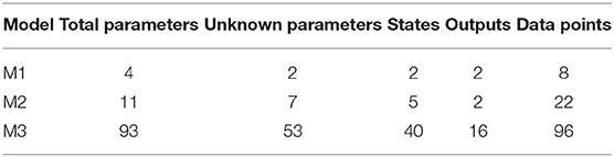
Table 2. Features of the models.

2.6. Lotka-Volterra Model (M1)

2.6.1. Model Description

The first model is the classical Lotka-Volterra model, which describes the interaction between the prey species x₁ and the predator species x₂ through the parameters a and b:

$\begin{array}{ll}\begin{array}{c}{ẋ}_1(a,t)=a{x}_1(t)-x_1(t)x_2(t),x_1(0)=1,\hfill \\ {ẋ}_2(b,t)=b{x}_1(t)x_2(t)-x_2(t),x_2(0)=0.5,\hfill \\ y(a,b,t)=\left[x_1(t),x_2(t)\right].\hfill \end{array}\hfill & (18)\end{array}$

The model parameter vector to estimate is p = [a, b], p ∈ ℝ². Both nominal values of parameters are set to 1. The observables are both variables x₁ and x₂.

To calibrate the model, we generate an in silico noisy dataset in the same way described by [35], i.e., sampling eight values of the output variables at the same specified time points and adding Gaussian noise ${N}(0,(0.5^2))$ (Table S1). Simulating the measurement noise with Gaussian noise is standard practice in mathematical modeling [5, 12, 35].

2.6.2. CRC Results

The tuning parameters of CRC are set as follows:

• the number of fixed samples in the parameter space is set to $N_S=10^4$ for each iteration;

• Equation (7) ∀i = 1, …2 is chosen as distance function between experimental and simulated data;

• the prior distributions for a and b are taken to be log-uniform: a, b ~ log −U(0.1, 10);

• k_U,1 = k_L,1 = 1 and k_U,2 = k_L,2 = 2 in all iterations.

According to Equation (7), the distance between the noisy dataset and the nominal solution is 3.09 for species x₁ and 2.6 for species x₂. Thus, the objective of the calibration is to obtain realizations of D_x1 and D_x2 that are close, respectively, to 3.09 and to 2.6. For this reason, the algorithm terminates when the two corresponding thresholds become sufficiently close to these two values. In order to do that, we perform six iterations of CRC. In the sixth iteration ${ϵ}_{x_1}^6$ and ${ϵ}_{x_2}^6$ are very close to the reference values presented above (3.09 and 2.6). This demonstrates that CRC reaches the desired level of agreement between simulated and experimental data. Table 3 sums up the tuning parameters and the results of CRC along the six iterations.

TABLE 3

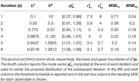
Table 3. Tuning parameters and results of CRC in model M1.

Figures 2A,B display the time behavior of output variables x₁ and x₂ when parameters belong to the final subset $P_{S,{ϵ}^6}$. The model simulations are shown together with the noisy dataset, proving both the validity and robustness of the solution. Figure 2C shows how the subset of accepted particles $P_{S,{ϵ}^z}$ changes during the execution of CRC.

FIGURE 2

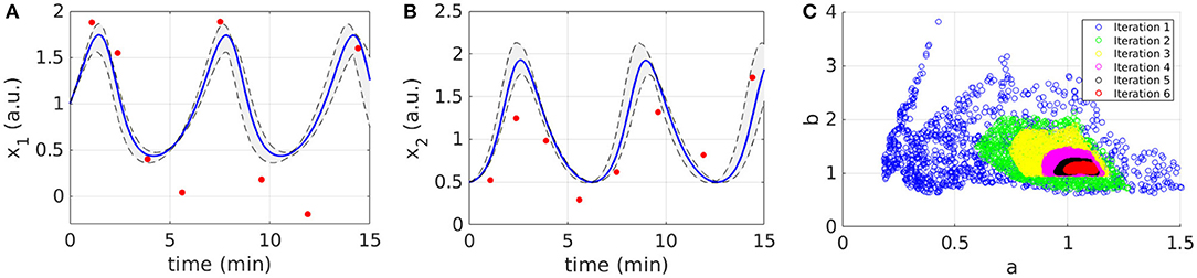
Figure 2. Results of CRC for model M1. (A,B) The red line is the time behavior of output variables when the parameter vector is equal to ${\text{p}}_m^6$ (see Table 3); red dots are the experimental data; the gray area represents the uncertainty in the temporal behavior of observables when parameters vary between the 2.5th and 97.5th percentile of their corresponding conditional pdfs. (C) Scatter plot of the sample distribution of $f_{a|P_{S,{ϵ}^z}(a)}$ (x-axis) vs. $f_{b|P_{S,{ϵ}^z}(b)}$ (y-axis) in all iterations.

CRC is fast in model calibration since the time simulation decreases from 288 s for the first iteration until 202 s for the last one. After model calibration, the CRA is applied in order to compute MIRIs for the parameters. We perturb the mode vector ${\text{p}}_m^{\zeta }=\left[1.06,1.06\right]$ generating 10⁴ samples of the parameter space. The lower and upper boundaries of the sampling are fixed equal to 0.1 and 10 and the probabilities β and λ are both fixed to 0.1, following the guidelines in [22]. For both parameters, we obtain that MIRIs have values around 1, meaning that a and b have approximately the same influence on the two output variables (Figure S3).

2.6.3. PL Results

First of all, we estimate parameter values using three different optimization algorithms, available in the software D2D [13]: lsqnonlin, genetic algorithms (GA), and simulated annealing (SA). In this example, both the default lsqnonlin and GA correctly fit the model yielding the same results, while SA totally fails in parameter estimation. The default method lsqnonlin estimates parameter a equal to 1.07 and parameter b equal to 1.05. Using these parameter values, the MSE is equal, respectively, to 0.19 for x₁ and to 0.13 for x₂. In order to evaluate the identifiability of model parameters and to assess their confidence intervals, we also calculate the PL. All tuning parameters of the algorithm are left to their default values. PL estimates as identifiable both model parameters (Figure S5). PL employs few seconds for parameter estimation and less than a minute for identifiability analysis of both parameters.

2.6.4. ABC-SMC Results

The application of the standard ABC-SMC method to the M1 model and the results obtained are comprehensively explained in [35]. In five steps the procedure converges to the considered threshold. In the 5-th iteration, parameter a has a median of 1.05 and a 95% interquartile range of [1, 1.12] whiifble parameter b has a median of 1 and a 95% interquartile range of [0.87, 1.11] [35]. When parameters are equal to their median values, MSE_x1 is 0.28 and MSE_x2 is 0.19.

2.6.5. DRAM Results

We apply DRAM to the M1 model varying the initial parameter values in the interval [0, 10], the initial error variance in the interval [0.01, 1] and the corresponding prior weight in the interval [1, 5]. The error variance is then estimated by setting options.updatesigma = 1. Moreover, in order to perform a reliable comparison with CRC, we set the number of simulations equal to 10⁴ and the boundaries of the parameters between [0, 10]. In all cases, the chains are stable and close to the nominal parameter values after one run. For the sake of brevity, we show only the results for initial error variance set to 0.1, prior weight set to 3 and initial parameter values equal to 0, 5, and 10. The time employed to apply the algorithm on the M1 model is about 3 minutes. Detailed results of DRAM are in S1 File.

2.7. EpoR System (M2)

2.7.1. Model Description

The ODE model presented in this section is taken from the Erythropoietin Receptor (EpoR) [44]. The model represents the catalysation of a substrate S by an enzyme E that is activated via two steps by an external ligand L [45]. This reaction cascade produces a product P whose dynamical behavior is the purpose of the model prediction. Generally the concentration over the time of the product P cannot be measured directly. Let denote with $\text{p}=\left[k_1,k_2,k_3,ini{t}_E,ini{t}_S,scal{e}_E,scal{e}_S\right],\text{p}\in {ℝ}^7$, the set of parameter to estimate. The nominal values of model parameters are p = [0.1, 0.1, 0.1, 10, 5, 4, 2]. The equations of the model, the corresponding initial conditions and the observables together with the dataset used for model calibration are reported in S1 File.

2.7.2. CRC Results

The prior distributions for all the model parameters are supposed log-uniform with the lower and upper boundaries set equal to L¹ = 0.01 and U¹ = 100. The number of fixed samples in the parameter space is $N_S=10^5$. We choose Equation (7) as distance function to evaluate the error between nominal and noisy data for the outputs of the model. According to the selected distance function, the errors between the nominal data points and the experimental ones are equal to 12.78 for y₁ and 5.6 for y₂. They represent the target thresholds to reach at the end of the last iteration in order to assert the success of CRC. To this purpose, we perform nine iterations of CRC in order to make the two thresholds close enough to their corresponding target values. Table 4 shows the boundaries of the proposal distribution in each iteration. These values are obtained by setting k_U,1 = k_L,1 = 0, k_U,2 = 2, and k_L,2 = 0.5 for the first seven iterations and k_U,1 = k_L,1 = 1 and k_U,2 = k_L,2 = 2 for the eighth and ninth iterations. Table 4 also shows the obtained thresholds for each performed iteration of CRC.

TABLE 4

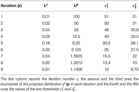
Table 4. CRC parameters for model M2.

In the ninth iteration, ${ϵ}_1^9$ and ${ϵ}_2^9$ are very similar to the target values presented above. This proves that CRC estimates a parameter vector that guarantees the desired level of agreement between simulated and experimental data. The mode vector in output from CRC is ${\text{p}}_m^{\zeta }=\left[0.11,0.02,0.08,34.93,2.99,1.12,3.37\right]$. The model simulation using as parameter vector the mode ${\text{p}}_m^{\zeta }$ has an MSE of 18.24 and 0.32 for y₁ and y₂ respectively. Figures 3A,B show the time behavior of both output variables when the parameter vector is set equal to the mode ${\text{p}}_m^{\zeta }$.

FIGURE 3

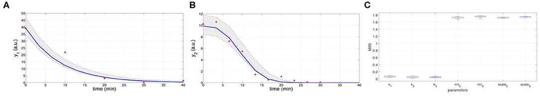
Figure 3. Results of CRC for model M2. (A,B) Time behavior of output variables. Red dots are the noisy experimental data [45]; blue lines are the simulations of the observables of the model when the parameter vector is set equal to the mode ${\text{p}}_m^{\zeta }$; gray regions are the confidence bands when parameter values are chosen between the 2.5-th and 97.5-th percentile of their corresponding conditional pdfs $f_{\text{P}|P_{S,{ϵ}^9}}$(p). (C) Boxplots of the MIRIs in output from the CRA for the seven model parameters and all the 10 independent realizations.

Moreover, regions in gray are the confidence bands of observables when parameter values are chosen between the 2.5-th and 97.5-th percentile of their corresponding conditional pdfs $f_{\text{P}|P_{S,{ϵ}^9}}(\text{p})$. In S1 File, additional details of f_Dy1(d_{y1, p}) and f_Dy2(d_{y2, p}) and the estimated conditional pdfs of parameters are reported. CRC is quite fast since it employs about 8 min (527 s) to complete one iteration.

Once the model has been correctly calibrated, we perform a robustness analysis in order to find those parameters that most affect the behavior of the output variables. We perturb the mode vector ${\text{p}}_m^{\zeta }$ with Linear LHS using 10⁵ samples. The lower and upper boundaries of the sampling are fixed equal to 0.01 and 100 respectively. Using the guidelines reported in [22] we fix the level of probabilities β and λ to 0.1. In Figure 3C the resulting MIRIs are shown. MIRIs corresponding to initial conditions parameters and scale factors are close to their maximum value and are much higher than those of the kinetic ones. This means that initial conditions and scale factors have major impact on observables compared to the kinetic parameters. We repeat the entire procedure ten times, obtaining ten independent realizations in order to ensure the invariance of results.

2.7.3. PL Results

The calculation of PL for M2 is presented in [45] where the authors reported that PL takes <1 min per parameter on a 1.8 GHz dual core machine. The parameter vector estimated through the PL is $\widehat{p}=\left[0.087,0.019,0.37,10.05,4.97,4.027,2.1\right]$. The MSE obtained through the PL approach is 10.06 and 0.3 for y₁ and y₂, respectively. As regards the identifiability analysis, according to the PL approach, parameter k₂ is classified as structurally non-identifiable, parameter k₃ is practically non-identifiable and the others are assessed to be identifiable. More details of the PL results are provided in S1 File.

2.7.4. ABC-SMC Results

ABC-SMC input parameters are set in order to resemble those of CRC. The distance function is defined as:

$\begin{array}{ll}d((y_1,y_2),(y_1^{*},y_2^{*}))={\displaystyle \sum _{i=1}^2}{\displaystyle \sum _{j=1}^{11}}|y_i(t_j)-y_{ij}^{*}|={\displaystyle \sum _{i=1}^2}AD{F}_i.& (19)\end{array}$

Under the hypothesis of parameters having a prior uniform distribution in [0, 100], we try to perform nine iterations of ABC-SMC. Thus, we set f_P(p) = U(0, 100) and z = 1, …, 9. The thresholds for all the iterations are chosen as the sum, over y₁ and y₂, of the two corresponding thresholds obtained from the application of CRC (Table 4). At each iteration, we select 1,000 particles of the parameter space under the desired threshold. The algorithm could not come to an end in a reasonable time and it finds parameter samples only until the 7-th iteration. In order to quantify the precision of the ABC-SMC approach, we perform simulations of the model, setting the parameter vector equal to the median of the ABC-SMC results. The MSE using these parameter values is 103 and 20 for y₁ and y₂, respectively. Further results of ABC-SMC are shown in S1 File.

2.7.5. DRAM Results

As in model M1, we run DRAM varying the initial error variance between [0.001,1] and the corresponding prior weight between [1, 5], and then we sample and estimate the error variance. Initial conditions were chosen close to nominal parameter values, i.e., [0.5, 0.5, 0.5, 8, 7, 5, 3]. As in CRC, the number of simulations is set to 10⁵, the number of run performed is nine and the parameter boundaries are [0, 100]. We run DRAM using, in one case, a Gaussian prior for all parameters and, in the other case, a lognormal prior. DRAM results are fairly stable against the different values of the initial error variance and the prior distribution. The chains of the first three parameters, k₁, k₂, and k₃, equally span all the values in the interval [0, 100] and accordingly the pdfs for those parameters are almost uniformly distributed, meaning that this parameters are classified as non identifiable. On the other hand, the chains corresponding to the other model parameters converge and are stable around specific values. This is also clearer from the corresponding pdfs that show a peak around the estimated value. Here, we report the results obtained in the final run with a lognormal prior, a prior weight set to 1 and an initial error variance that varies between 0.001 and 1. DRAM employs about 15 min to complete one run. In S1 File, figures of DRAM results are provided.

2.8. Multiple Myeloma Model (M3)

2.8.1. Model Description

M3 is the ODE model proposed in [46]. The mathematical model is defined to help study the roles that various p38 MAPK isoforms play in MM. It has 40 ODEs, built using only the law of mass action, and 53 kinetic parameters (S1 File). According to Peng et al. [46], data associated to the model are the output of a Reverse Phase Protein Array (RPPA) experiment [2], where MM cell lines were analyzed to detect the activity of proteins active in various p38 MAPK signaling pathways. RPPA was performed on the following cell lines: four different RPMI 8226 MM cell sublines with stable silenced expression of p38α, p38β, p38γ, and p38δ, respectively, as well as an RPMI 8226 MM stable cell subline transfected with empty vector as the negative control. Cells were treated with arsenic trioxide (ATO), bortezomib (BZM) or their combination. RPPA analyzed a total of 80 samples and measured 153 proteins at six different time points. The proteins whose phosporylation level was included both in the pathway and in the experiment are 16. All RPPA data are normalized based on the initial concentration value. For this reason, initial conditions of proteins in the ODE model are all set to 1, i.e., x(0)=1. Parameters to estimate are only the kinetic ones, i.e., p ∈ ℝ⁵³. In [46], available data for model calibration belongs to the p38δ knockdown cell line treated with BZM. The corresponding RPPA dataset is presented in Table S13.

2.8.2. CRC Results

For model M3, we set tuning parameters of CRC in the following way:

• the number of parameter samples N_S is equal to 10⁶;

• for each output variable, Equation (8) is chosen as distance function;

• the prior of each kinetic parameter is supposed to be log − U(0.1, 10);

• k_U,1 = k_L,1 = 1 and k_U,2 = k_L,2 = 2 in all iterations.

Six iterations of CRC are performed, using the threshold schedule reported in Table 5. At the end of the process, the maximum error between simulated and experimental data is only of the 16%.

TABLE 5

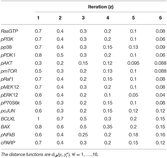
Table 5. Threshold schedule of distance functions for model M3.

Figure 4A shows the time behavior of output variables at the end of the calibration, along with experimental data points. The figure proves that the algorithm is successful in finding a robust solution (S1 File). As regards the application of CRA, we perturb the parameter space in the interval having as lower and upper boundaries 0.01 and 100, respectively and centered around the final mode vector ${\text{p}}_m^6$, generating 10⁶ parameter samples. In Figure 4B, MIRIs are presented for each parameter. As expected, not all parameters have a strong impact on the observables since the number of output variables is small compared to all kinetic parameters. For instance, parameters k_{Raf1_pPI3K}, k_{ERK12_pp38}, k_{BAX_pp38}, k_{IKK_pAKT}, k_{PARP_BAX}, k_{cPARP_BCLXL} have all a MIRI value under 0.2. On the other hand, about a fifth of the total number of parameters has MIRI values above 1.6 (e.g., parameters k_GFR, k_pGFR, k_{Shc_pGFR}, k_pPI3K, k_pAKT, k_{pRaf1_pAkt}, k_pMEK12, k_{ERK12_MEK12}, k_pERK12, k_pP70S6K, k_pJNK), meaning that they have high influence on the outputs. We repeat the entire procedure ten times, obtaining ten independent realizations in order to ensure the invariance of results.

FIGURE 4

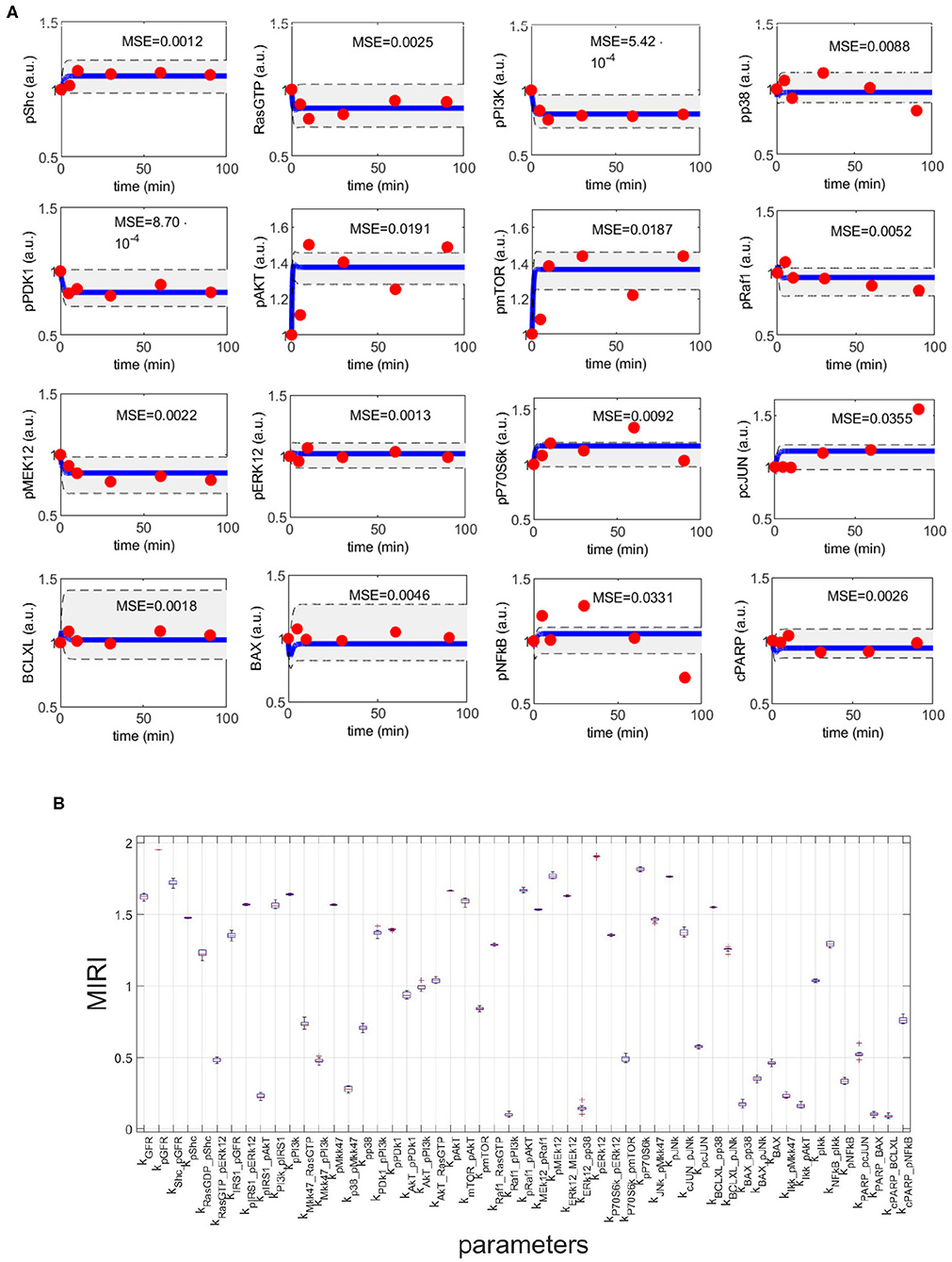
Figure 4. CRC results for model M3. (A) The blue line is the time behavior of observables when the parameter vector is equal to ${\text{p}}_m^6$ (see Table S25); red dots are the RPPA data [46]; the gray area reproduces the variation of the temporal behavior when parameters vary between the 2.5-th and 97.5-th percentile of their corresponding conditional pdfs $f_{\text{P}|P_{S,{ϵ}^6}}(\text{p})$. On the top of each plot, the MSE between the associated model simulation and the data is reported. (B) Boxplot of MIRIs for the estimated parameter values, along the 10 independent realizations performed.

2.8.3. PL Results

First of all, through the D2D software, we calibrate the model using lsqnonlin as optimization algorithm. To avoid local optima, we execute a sequence of n = 100 fits using LHS. Moreover, we also estimate model parameters using GA and SA. While GA is not able to correctly reproduce experimental data, SA successfully estimates the time behavior of output variables. To compute confidence intervals, the maximum number of sampling steps in both the increasing and decreasing direction of each parameter is set to 200 while all the other tuning parameters of the method are set to their default values. The upper and lower boundaries of the parameter prior are set respectively to 10⁻⁵ and 10³. Results of parameter estimation and identifiability analysis are shown in S1 File. The algorithm assesses that all parameters are identifiable except for the following parameters: k_{P70S6K_pERK12}, k_{cPARP_BCLXL}, k_pJNK that are practically non-identifiable and k_{pIRS1_pAKT} is structurally non-identifiable. Nevertheless, the results obtained are not so reliable since some parameters have a confidence interval of only a single value (e.g., k_{IRS1_pGFR}) while others have an estimated value outside the corresponding confidence region (e.g., k_{PDK1_pPI3K}). The PL algorithm employs less than one minute for parameter estimation and about 40 min for identifiability analysis of all parameters.

2.8.4. ABC-SMC Results

Using the ABC-SysBio software, we fix ABC-SMC parameters as follows:

• the distance function is defined as:

$\begin{array}{ll}d(y,y^{*})=\frac{1}{6}{\displaystyle \sum _{i=1}^{16}}{\displaystyle \sum _{j=1}^6}\frac{|y_i(t_j)-y_{ij}^{*}|}{y_{ij}^{*}}={\displaystyle \sum _{i=1}^{16}}AND{F}_i;& (20)\end{array}$

• the number of iterations is set to 6;

• the threshold fixed in each iteration is equal to the sum of all thresholds fixed in CRC in the same iteration (see Table S29);

• the number of accepted particles at each iteration is set to 1,000;

• all parameters to estimate are supposed to have a uniform prior distribution: U(0.1,10);

• all the other parameters are left to their default values.

The application of ABC-SMC to the M3 model was very time consuming and, after 10 days, it had not converged yet. Thus, results are available only until the 4-th iteration (see S1 File).

2.8.5. DRAM Results

As in the previous examples, we run DRAM setting the number of simulations equal to those of CRC (10⁶) and the number of run to six. The initial error variance, that is estimated, and the corresponding prior weight are set equal to 0.1 and 10, respectively. Initial values of parameters are all equal to 1 and the parameter boundaries are [0, 10]. We run DRAM using both a uniform and lognormal prior for all parameters. DRAM employs about 3 h to complete one run and, in the end, most parameters have a uniform distribution. In S1 File, we provide figures of DRAM results after six run with a lognormal prior. We show the chains and pdfs of the parameters and the time simulations of the output variables of the model when parameters are equal to mean of the corresponding chains.

3. Discussion

Here we present a novel Bayesian approach for parameter estimation of mathematical models that is used to fit omics data in Systems Biology applications. The availability of high-throughput data with the need to calibrate high dimensional models using computational feasible algorithms, makes CRC a useful and innovative procedure in the overview of the Bayesian parameter estimation and robustness analysis. Our algorithm modifies the standard ABC-SMC in order to increase the efficiency and the reliability of the estimated parameter vector. Moreover, CRC presents many distinctive improvements as compared to other algorithms of the ABC-SMC family, such as ABC-PMC and Adaptive-ABC [21].

We validated this new methodology in three ODE models, each one with specific features, in order to demonstrate the flexibility and reliability of our approach. In addition, we compared CRC results with those obtained by methods representing the state of the art of this field, i.e., the standard ABC-SMC, PL, and DRAM. Table 6 summarizes the comparison between CRC and the other benchmarking algorithms tested.

TABLE 6

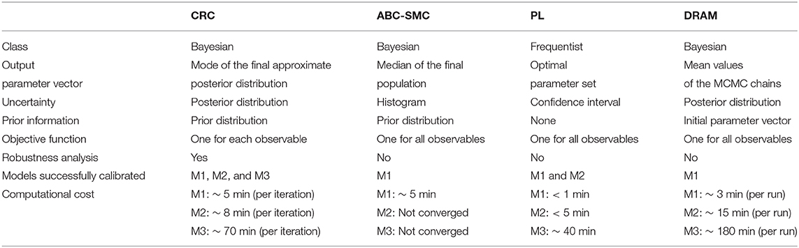
Table 6. Comparison between parameter estimation algorithms.

First of all, we tested all the calibration procedures in the Lotka-Volterra model. We showed that all algorithms performed well, but with some differences. CRC returns a reliable and robust solution. Compared with ABC-SMC, we performed one more iteration but the computational burden was almost irrelevant since each iteration took about 5 min to complete. CRC also finds a more precise solution and generates a remarkable minor number of particles for sampling the parameter space. PL succeeds in fitting the data when lsqnonlin and GA are used. Then, through confidence intervals, it classifies both parameters as identifiable, in accordance with MIRI values. DRAM, after the initial adaptation period, finds acceptable points and a good mixing of the chain, regardless of the choice for the tuning parameter values.

Next we compared the results of CRC in the model presented in [44, 45]. In this example, CRC finds an alternative solution of the parameter vector compared to that of PL. PL fits the data properly and fast and identifiability results are in accordance with MIRI values. ABC-SMC fails in the calibration procedure and it cannot go beyond the 7-th iteration, proving that it cannot reach an error as low as the one of CRC. As regards DRAM, the final results are in agreement with those of CRC. The chains of parameters are not significantly affected by the variation of the tuning parameters and, for most of them, the chains converged generating a peak in the corresponding pdf. For the first three kinetic parameters the estimated posterior pdfs are uniformly distributed since the chains equally span all the interval, meaning that they are non identifiable. As for CRC, DRAM finds a different solution for the parameter vector. However, the parameter vector estimated by DRAM is not able to produce reliable time behaviors of the output variables and as a consequence the experimental data feed to DRAM are not well-recapitulated by the time behavior of the observables. This is mainly due to the fact that in the given dataset there are many missing values and DRAM filtered out all the observations with at least one missing value. So the poor results in terms of time behavior are not due to a lack of the algorithm itself but mainly because it cannot deal with missing values, contrary to the other benchmarking algorithms presented in this paper.

Finally, the last model is an high-dimensional ODE model calibrated on real experimental data [46]. CRC was able to find a set of parameter vectors that fit well experimental data. In addition, robustness analysis highlights that about half of the parameters influences most output variables. PL is successful in model calibration but computation of confidence intervals gives confounding results which do not allow a reliable comparison with MIRI values. ABC-SMC fails in model calibration because it remains blocked in the 5-th out of 6 iterations. Also DRAM does not find a reliable solution since all the parameter chains are not stable and, after 10⁶ simulations, they span the interval [0, 10] almost uniformly. Moreover, compared to CRC, it has an higher computational cost.

In summary, the main disadvantage of the standard ABC-SMC method is the time necessary to complete a simulation which increases with the model dimension. The PL method is fast in model calibration even for high dimensional models since it implements an optimization algorithm. However, the returned solution does not contain any information on the distribution of parameters since it represents a single point in the parameter space. Moreover, as shown in model M3, it may return improper results in the computation of parameter profiles. As regards DRAM, its results are highly affected by the initial values of the parameters, which must be set from the beginning. This point is crucial since in Systems Biology models most parameter values are unknown and cannot be measured experimentally.

CRC is able to identify a stable and precise solution in all test models, mainly because of some of distinctive features. One of its main innovations is the use of a fixed number of points for sampling the parameter space, which is initially chosen by the user and does not change throughout iterations. As a result, the model is always integrated N_S times in each iteration. Since most of the computational cost of an iteration of CRC is given by the integration of the model, CRC guarantees a limited computational cost through the different iterations. On the other hand, in other ABC-SMC methods, the computational burden is substantial because the number of samples at each iteration is not known a priori but strictly depends on the threshold value. Since the threshold usually decreases at each step, the number of generated samples could increase together with the simulation time. However, compared to the frequentist approach, CRC has always an higher computational cost since it requires multiple subsequent iterations and multiple integrations of the model in order to converge toward the final solution.

Moreover, another significant innovation introduced is the definition of an objective function for each output variable. This allows a model calibration that takes equally into account all experimental endpoints. On the other hand, the other techniques evaluate only a single and unique objective function, which includes information about all observables. Even if the introduction of multiple objective functions improves the accuracy and the performances of CRC, it requires multiple thresholds to be chosen by the user, at each iteration. As a consequence, different combinations of the values of thresholds could guarantee the fulfillment of the two constraints explained in section 2.3.1 (${ϵ}_i^z\le {ϵ}_i^{z-1}$ and $|P_{S,{ϵ}^z}|>1000$). In order to overcome this drawback of CRC, it is possible to implement an optimization strategy step that automatically computes, at each iteration, the minimum value of each threshold that satisfies the constraints explained above and potentially further policies defined by the user. This disadvantage of CRC becomes more relevant in models with an high number of output variables to calibrate.

Finally, we also analyzed the robustness of model parameters in a new way, taking inspiration from the CRA presented in [22]. This algorithm is based on the concept of robustness proposed by Kitano [47], which defines it as the property of a system to maintain its status against internal and external perturbations. We employed CRA in order to quantify the robustness of the model observables against the simultaneous perturbation of the parameters.

Robustness analysis is useful for applications in cancer drug discovery aimed at finding which node of a network could be identified as novel potential drug target. Moreover, the concept of robustness is slightly different from that of identifiability introduced with the PL approach. A parameter that is declared identifiable should have an high MIRI value since it has great impact on the outputs behavior. On the other hand, if a parameter is non-identifiable it is impossible to understand its influence on the observables dynamical response, without performing our robustness analysis. While ABC-SMC evaluates parameter identifiability only through histograms of final parameter values and DRAM computes the parameter posterior distribution, CRC estimates conditional parameter densities, and performs robustness analysis through the MIRI indicator that quantifies the influence of each parameter on the behavior of interest. Indeed, the higher the MIRI value the higher the impact of the parameter on the entire set of observables. All the innovations introduced with CRC are important for a successful calibration of high dimensional nonlinear models in Systems Biology applications based on omics data.

Data Availability Statement

The datasets generated for this study can be found in the https://github.com/fortunatobianconi/CRC.

Author Contributions

FB, CA, and LT conceived and designed the methods. FB, CA, LT, and PV designed computational benchmark experiments and wrote the paper. CA and LT performed computational analysis. All authors reviewed the manuscript.

Funding

This study was supported by the Italian Association for Cancer Research (AIRC) grant (15713/2014).

Conflict of Interest

The authors declare that the research was conducted in the absence of any commercial or financial relationships that could be construed as a potential conflict of interest.

Acknowledgments

This manuscript has been released as a Pre-Print at [48].

Supplementary Material

The Supplementary Material for this article can be found online at: https://www.frontiersin.org/articles/10.3389/fams.2020.00025/full#supplementary-material

S1 File. For each model, equations and data are shown together with additional tables and figures of the results.

References

1. Ludovini V, Bianconi F, Siggillino A, Piobbico D, Vannucci J, Metro G, et al. Gene identification for risk of relapse in stage I lung adenocarcinoma patients: a combined methodology of gene expression profiling and computational gene network analysis. Oncotarget. (2016) 7:30561–74. doi: 10.18632/oncotarget.8723

CrossRef Full Text | Google Scholar

2. Ludovini V, Chiari R, Tomassoni L, Antonini C, Baldelli E, Baglivo S, et al. Reverse phase protein array (RPPA) combined with computational analysis to unravel relevant prognostic factors in non- small cell lung cancer (NSCLC): a pilot study. Oncotarget. (2017) 8:83343–53. doi: 10.18632/oncotarget.18480

PubMed Abstract | CrossRef Full Text | Google Scholar

3. Motta S, Pappalardo F. Mathematical modeling of biological systems. Brief Bioinformatics. (2012) 14:411–22. doi: 10.1093/bib/bbs061

CrossRef Full Text | Google Scholar

4. Bartocci E, Lió P. Computational modeling, formal analysis, and tools for systems biology. PLoS Comput Biol. (2016) 12:e1004591. doi: 10.1371/journal.pcbi.1004591

PubMed Abstract | CrossRef Full Text | Google Scholar

5. Lillacci G, Khammash M. Parameter estimation and model selection in computational biology. PLoS Comput Biol. (2010) 6:e1000696. doi: 10.1371/journal.pcbi.1000696

PubMed Abstract | CrossRef Full Text | Google Scholar

6. Machado D, Costa RS, Rocha M, Ferreira EC, Tidor B, Rocha I. Modeling formalisms in systems biology. AMB Express. (2011) 1:45. doi: 10.1186/2191-0855-1-45

PubMed Abstract | CrossRef Full Text

7. Kitano H. Systems biology: a brief overview. Science. (2002) 295:1662–64. doi: 10.1126/science.1069492

PubMed Abstract | CrossRef Full Text | Google Scholar

8. Alon U. An Introduction to Systems Biology : Design Principles of Biological Circuits. Boca Raton, FL: Chapman & Hall; CRC Press (2007).

Google Scholar

9. Penas DR, González P, Egea JA, Doallo R, Banga JR. Parameter estimation in large-scale systems biology models: a parallel and self-adaptive cooperative strategy. BMC Bioinformatics. (2017) 18:52. doi: 10.1186/s12859-016-1452-4

PubMed Abstract | CrossRef Full Text | Google Scholar

10. Fröhlich F, Kaltenbacher B, Theis FJ, Hasenauer J. Scalable parameter estimation for genome-scale biochemical reaction networks. PLoS Comput Biol. (2017) 13:e1005331. doi: 10.1371/journal.pcbi.1005331

PubMed Abstract | CrossRef Full Text | Google Scholar

11. Degasperi A, Fey D, Kholodenko BN. Performance of objective functions and optimisation procedures for parameter estimation in system biology models. NPJ Syst Biol Appl. (2017) 3:20. doi: 10.1038/s41540-017-0023-2

PubMed Abstract | CrossRef Full Text | Google Scholar

12. Vanlier J, Tiemann CA, Hilbers PAJ, van Riel NAW. Parameter uncertainty in biochemical models described by ordinary differential equations. Math Biosci. (2013) 246:305–14. doi: 10.1016/j.mbs.2013.03.006

PubMed Abstract | CrossRef Full Text | Google Scholar

13. Raue A, Schilling M, Bachmann J, Matteson A, Schelke M, Kaschek D, et al. Lessons learned from quantitative dynamical modeling in systems biology. PLoS ONE. (2013) 8:e74335. doi: 10.1371/journal.pone.0074335

PubMed Abstract | CrossRef Full Text | Google Scholar

14. Raue A, Kreutz C, Maiwald T, Bachmann J, Schilling M, Klingmüller U, et al. Structural and practical identifiability analysis of partially observed dynamical models by exploiting the profile likelihood. Bioinformatics. (2009) 25:1923–9. doi: 10.1093/bioinformatics/btp358

PubMed Abstract | CrossRef Full Text | Google Scholar

15. Thomaseth K, Saccomani MP. Local identifiability analysis of nonlinear ODE models: how to determine all candidate solutions. IFAC-PapersOnLine. (2018) 51:529–34. doi: 10.1016/j.ifacol.2018.03.089

CrossRef Full Text | Google Scholar

16. Raue A, Karlsson J, Saccomani MP, Jirstrand M, Timmer J. Comparison of approaches for parameter identifiability analysis of biological systems. Bioinformatics. (2014) 30:1440–8. doi: 10.1093/bioinformatics/btu006

PubMed Abstract | CrossRef Full Text | Google Scholar

17. Wilkinson DJ. Bayesian methods in bioinformatics and computational systems biology. Brief Bioinformatics. (2006) 8:109–16. doi: 10.1093/bib/bbm007

CrossRef Full Text | Google Scholar

18. Sunnåker M, Busetto AG, Numminen E, Corander J, Foll M, Dessimoz C. Approximate Bayesian computation. PLoS Comput Biol. (2013) 9:e1002803. doi: 10.1371/journal.pcbi.1002803

PubMed Abstract | CrossRef Full Text | Google Scholar

19. Liepe J, Kirk P, Filippi S, Toni T, Barnes CP, Stumpf MPH. A framework for parameter estimation and model selection from experimental data in systems biology using approximate Bayesian computation. Nat Protoc. (2014) 9:439–56. doi: 10.1038/nprot.2014.025

PubMed Abstract | CrossRef Full Text | Google Scholar

20. Brooks S. Markov chain Monte Carlo method and its application. J R Stat Soc Ser D. (1998) 47:69–100. doi: 10.1111/1467-9884.00117

CrossRef Full Text | Google Scholar

21. Prangle D, et al. Adapting the ABC distance function. Bayesian Anal. (2017) 12:289–309. doi: 10.1214/16-BA1002

CrossRef Full Text | Google Scholar

22. Bianconi F, Baldelli E, Luovini V, Petricoin EF, Crinò L, Valigi P. Conditional robustness analysis for fragility discovery and target identification in biochemical networks and in cancer systems biology. BMC Syst Biol. (2015) 9:70. doi: 10.1186/s12918-015-0216-5

PubMed Abstract | CrossRef Full Text | Google Scholar

23. Raue A, Steiert B, Schelker M, Kreutz C, Maiwald T, Hass H, et al. Data2Dynamics: a modeling environment tailored to parameter estimation in dynamical systems. Bioinformatics. (2015) 31:3558–60. doi: 10.1093/bioinformatics/btv405

PubMed Abstract | CrossRef Full Text | Google Scholar

24. Haario H, Laine M, Mira A, Saksman E. DRAM: efficient adaptive MCMC. Stat Comput. (2006) 16:339–54. doi: 10.1007/s11222-006-9438-0

CrossRef Full Text | Google Scholar

25. Laine M. MCMC Toolbox for Matlab. (2018). Available online at: https://mjlaine.github.io/mcmcstat/

26. Martino L. A review of multiple try MCMC algorithms for signal processing. Digital Signal Process. (2018) 75:134–52. doi: 10.1016/j.dsp.2018.01.004

CrossRef Full Text | Google Scholar

27. Liu JS, Liang F, Wong WH. The multiple-try method and local optimization in Metropolis sampling. J Am Stat Assoc. (2000) 95:121–34. doi: 10.1080/01621459.2000.10473908

CrossRef Full Text | Google Scholar

28. Luengo D, Martino L. Fully adaptive gaussian mixture metropolis-hastings algorithm. In: 2013 IEEE International Conference on Acoustics, Speech and Signal Processing. Vancouver, BC (2013). p. 6148–52.

Google Scholar

29. Giordani P, Kohn R. Adaptive independent Metropolis–Hastings by fast estimation of mixtures of normals. J Comput Graph Stat. (2010) 19:243–59. doi: 10.1198/jcgs.2009.07174

CrossRef Full Text | Google Scholar

30. McKay MD, Beckman RJ, Conover WJ. A comparison of three methods for selecting values of input variables in the analysis of output from a computer code. Technometrics. (2000) 42:55–61. doi: 10.1080/00401706.2000.10485979

CrossRef Full Text | Google Scholar

31. Stein M. Large sample properties of simulations using Latin hypercube sampling. Technometrics. (1987) 29:143–51. doi: 10.1080/00401706.1987.10488205

CrossRef Full Text | Google Scholar

32. Wyss GD, Jorgensen KH. A Users Guide to LHS: Sandias Latin Hypercube Sampling Software. Albuquerque, NM: Sandia National Labs. (1998).

Google Scholar

33. Bianconi F, Antonini C, Tomassoni L, Valigi P. An application of Conditional Robust Calibration (CRC) to ordinary differential equations (ODEs) models in computational systems biology: a comparison of two sampling strategies. IET Syst Biol. (2019) 14:107–19. doi: 10.1049/iet-syb.2018.5091

PubMed Abstract | CrossRef Full Text | Google Scholar

34. Bianconi F, Baldelli E, Ludovini V, Crinò L, Perruccio K, Valigi P. Robustness of complex feedback systems: application to oncological biochemical networks. Int J Control. (2013) 86:1304–21. doi: 10.1080/00207179.2013.800646

CrossRef Full Text | Google Scholar

35. Toni T, Welch D, Strelkowa N, Ipsen A, Stumpf MPH. Approximate Bayesian computation scheme for parameter inference and model selection in dynamical systems. J R Soc Interface. (2009) 6:187–202. doi: 10.1098/rsif.2008.0172

PubMed Abstract | CrossRef Full Text | Google Scholar

36. Maier C, Loos C, Hasenauer J. Robust parameter estimation for dynamical systems from outlier-corrupted data. Bioinformatics. (2016) 33:718–25. doi: 10.1093/bioinformatics/btw703

PubMed Abstract | CrossRef Full Text | Google Scholar

37. Bianconi F, Antonini C, Tomassoni L, Valigi P. CRA toolbox: software package for conditional robustness analysis of cancer systems biology models in MATLAB. BMC Bioinformatics. (2019) 20:385. doi: 10.1186/s12859-019-2933-z

PubMed Abstract | CrossRef Full Text | Google Scholar

38. Beaumont MA, Zhang W, Balding DJ. Approximate Bayesian computation in population genetics. Genetics. (2002) 162:2025–35.

PubMed Abstract | Google Scholar

39. Marjoram P, Molitor J, Plagnol V, Tavaré S. Markov chain Monte Carlo without likelihoods. Proc Natl Acad Sci USA. (2003) 100:15324–8. doi: 10.1073/pnas.0306899100

PubMed Abstract | CrossRef Full Text | Google Scholar

40. McCall J. Genetic algorithms for modelling and optimisation. J Comput Appl Math. (2005) 184:205–22. doi: 10.1016/j.cam.2004.07.034

CrossRef Full Text | Google Scholar

41. Ingber L. Adaptive simulated annealing (ASA): lessons learned. Control Cybern. (1996) 25:33–54.

42. Robert CP, Richardson S. Markov chain Monte Carlo methods. In: Discretization and MCMC Convergence Assessment. New York, NY: Springer (1998). p. 1–25.

PubMed Abstract | Google Scholar

43. Green PJ, Mira A. Delayed rejection in reversible jump Metropolis–Hastings. Biometrika. (2001) 88:1035–53. doi: 10.1093/biomet/88.4.1035

CrossRef Full Text | Google Scholar

44. Becker V, Schilling M, Bachmann J, Baumann U, Raue A, Maiwald T, et al. Covering a broad dynamic range: information processing at the erythropoietin receptor. Science (2010) 328:1404–8. doi: 10.1126/science.1184913

PubMed Abstract | CrossRef Full Text | Google Scholar

45. Maiwald T, Timmer J, Kreutz C, Klingmüller U, Raue A. Addressing parameter identifiability by model-based experimentation. IET Syst Biol. (2011) 5:120–30. doi: 10.1049/iet-syb.2010.0061

PubMed Abstract | CrossRef Full Text | Google Scholar

46. Peng H, Peng T, Wen J, Engler DA, Matsunami RK, Su J, et al. Characterization of p38 MAPK isoforms for drug resistance study using systems biology approach. Bioinformatics. (2014) 30:1899–907. doi: 10.1093/bioinformatics/btu133

PubMed Abstract | CrossRef Full Text | Google Scholar

47. Kitano H. Towards a theory of biological robustness. Mol Syst Biol. (2007) 3:137. doi: 10.1038/msb4100179

PubMed Abstract | CrossRef Full Text | Google Scholar

48. Bianconi F, Tomassoni L, Antonini C, Valigi P. A new Bayesian methodology for nonlinear model calibration in Computational Systems Biology. BioRxiv [Preprint]. (2019). doi: 10.1101/633180

CrossRef Full Text | Google Scholar