A Scalar Poincaré Map for Anti-phase Bursting in Coupled Inhibitory Neurons With Synaptic Depression

1. Introduction

Short-term synaptic plasticity may have a role in burst activity in central pattern generators (CPGs). Short-term synaptic depression is commonly found in neuronal networks involved in the generation of rhythmic movements, such as in the pyloric CPG of the spiny lobster [1, 2], or in the lumbosacral cord of the chick embryo [3]. Synaptic depression modulates the strength of synapses in response to changes to the presynaptic firing frequency. At a high neuronal firing frequency, depression weakens the strength of synapses and therefore reduces the magnitude of the postsynaptic response. At low firing frequency, it allows sufficient time for the synapse to recover from depression between spikes, leading to a stronger postsynaptic response. In reciprocal networks, synaptic depression has been shown to act as a “switch,” giving rise to a wide range of network dynamics such as synchronous and multi-stable rhythms, as well as fine tuning the frequency of network oscillations [4–6].

Brown [7] pioneered the idea that synaptic depression acts as a burst termination mechanism in CPGs composed of reciprocally inhibitory neurons and involved in rhythm generation of locomotion. When one side is firing during a burst the other, antagonistic side, is prevented from firing by synaptic inhibition. However, the weakening of inhibition as a result of synaptic depression eventually releases the antagonistic side so that it starts firing, terminating the burst on the side that had originally been firing. This rhythmogenesis hypothesis has been considered one of a handful of standard mechanisms for generating locomotion rhythms in vertebrates [8–10]. It has been proposed as an explanation of the antiphase burst rhythm in struggling in Xenopus tadpoles [11].

Bose and Booth [6] investigated burst generation in a generic half-center CPG that consists of two identical, tonically active Morris-Lecar [12] neurons coupled through inhibitory depressing synapses. Numerical simulations showed that when the reciprocal synaptic conductance between the two neurons is varied, the network produces symmetric n : n anti-phase bursts, with stronger synaptic coupling leading to longer bursts. They used methods from geometric singular perturbation theory to separate the timescales of the fast membrane, and the slow synaptic dynamics of the network to derive one-dimensional conditions necessary for the existence of stable n : n solutions (for n ≤ 2). According to these conditions the type of firing pattern largely depends on the slow depression dynamics of the synapses between the two neurons, and can therefore be predicted by knowing the strengths of the synaptic conductances of the two synapses. Thus, the scalar conditions derived in Bose and Booth [6] provide a method to numerically identify the type of stable n : n pattern for any given value of the coupling strength and n ≤ 2. However, they do not predict the exact period of such solutions. Furthermore, while they provide good arguments for the validity of their reduction assumptions and the resulting scalar conditions, they do not verify them numerically.

Here we extend the previous analysis by providing a Poincaré map of the slow depression dynamics. This allows us not only to predict the types of stable n : n solutions the full network can produce, (for any n), but also to study how varying the coupling strength affects the period of such solutions. To do this, we build on, and numerically test, the assumptions on the fast-slow timescale disparity made in Bose and Booth [6]. We reduce the two-cell model to a scalar Poincaré map that tracks the evolution of the depression from the beginning of one burst to the beginning of the next burst. Stable fixed points of our map are associated with stable n : n burst solutions. Our map construction is motivated by the burst length map of a T-type calcium current, utilized by Matveev et al. [13], which approximates the anti-phase bursting dynamics of a network of two coupled Morris-Lecar neurons. In contrast to our model, the network described in the Matveev et al. [13] paper does not contain short-term synaptic depression, and burst termination is instead accomplished through the dynamics of a slow T-type calcium current.

The Poincaré map derived here replicates the results from numerical simulations of the full two-cell ODE system: Given the strength of maximum conductance between the two neurons, fixed points of our map predict the type and period of n : n patterns, the switch between burst solutions of different periods, as well as the occurrence of co-existent solutions. In addition to proving the existence and stability of fixed points, our map shows that fixed points are created via a fold bifurcation of maps. Finally, we use our map to derive algebraic conditions that allow us to predict parameter values of the maximum conductance at which n : n solutions bifurcate to (n + 1) : (n + 1) solutions, and vice versa. Because our map is fully explicit, it lays the framework for studying the effects of other model parameters on network dynamics without the need to run expensive numerical integrations of the ODEs.

This paper is organized as follows. First, we introduce the network of two neurons, and describe the properties of single cell and synapse dynamics. We use numerical simulations of the network to provide an intuition for the range of possible burst dynamics the system can produce. Next, we state and justify the simplifying assumptions that are necessary for the map construction. Finally, we analytically derive the first return map of the depression variable as well as the conditions that are required for stable n : n solutions. We end this work with a discussion.

2. Materials and Methods

We consider a pair of identical Morris-Lecar neurons [12], with parameters from Bose and Booth [6]. The Morris-Lecar model is a set of two first-order differential equations that describe the membrane dynamics of a spiking neuron. The depolarisation is modeled by an instantaneous calcium current, and the hyperpolarisation by a slow potassium current and a leak current. The membrane potential v_i and potassium activation w_i of neuron i (i, j = 1, 2) is described by:

$\begin{array}{ll}{\stackrel{.}{v}}_i=f(v_i,w_i)-\overline{g}{s}_j(v_i-v_s),& (1)\end{array}$

$\begin{array}{ll}{\stackrel{.}{w}}_i=h(v_i,w_i).& (2)\end{array}$

Here v_s is the inhibitory reversal potential, and $\overline{g}$ and s_j are the maximal synaptic conductance and the synaptic gating, respectively, constituting the total inhibitory conductance $\overline{g}$s_j from neuron j to neuron i. Function f(v_i, w_i) describes the membrane currents of a single cell:

$\begin{array}{l}f(v_i,w_i)=-g_{\text{Ca}}{m}_{\infty }(v_i)(v_i-v_{\text{Ca}})-g_{\text{K}}{w}_i(v_i-v_{\text{K}})\\ -g_{\text{L}}(v_i-v_{\text{L}})+I.& (3)\end{array}$

The currents include a constant current I, and three ionic currents: an instantaneous calcium current, a potassium current, and a leak current, with respective reversal potentials v_Ca, v_K, and v_L, as well as maximum conductances g_Ca, g_K, and g_L. The function h(v_i, w_i) models the kinetics of the potassium gating variable w_i, and is given by

$\begin{array}{ll}h(v_i,w_i)=\frac{w_{\infty }(v_i)-w_i}{{\tau }_w}.& (4)\end{array}$

The steady-state activation functions m_∞ and w_∞ as well as the default model parameters are described in the Supplementary Material 1.

The dynamics of the synaptic interactions between the neurons are governed by a synaptic gating variable s_i and a depression variable d_i:

$\begin{array}{ll}{\stackrel{.}{d}}_i=\{\begin{array}{ll}(1-d_i)/{\tau }_a& if{v}_i<v_{\theta },\\ -d_i/{\tau }_b& if{v}_i>v_{\theta },\end{array}& (5)\end{array}$

$\begin{array}{ll}{\stackrel{.}{s}}_i=\{\begin{array}{ll}-s_i/{\tau }_{\kappa }& if{v}_i<v_{\theta },\\ 0& if{v}_i>v_{\theta }.\end{array}& (6)\end{array}$

Variable d_i describes a firing rate dependent depletion mechanism that governs the amount of depression acting on the synapse. The model is agnostic with respect to the exact mechanism of this depletion, be it pre- or post-synaptic. When the voltage of cell i is above firing threshold (v_i > v_θ), variable d_i decays with time constant τ_b, and recovers with time constant τ_a when voltage is below firing threshold (v_i < v_θ). Since the synaptic inhibition occurs on a much faster timescale than synaptic depression, we assume that s_i is instantaneously reset to d_i whenever v_i increases above v_θ, where it remains throughout v_i > v_θ. Whenever v_i < v_θ, the synaptic variable decays exponentially with time constant τ_κ. The equations for the depression model are identical to the Bose and Booth [14] model. These equations are a mathematically tractable simplification of the established phenomenological depression model previously described by Tsodyks and Markram [15].

When the total inhibitory conductance $\overline{g}$s_j is constant, the membrane dynamics are determined by the cubic v-nullcline v_∞(v_i) and the sigmoid w-nullcline w_∞(v_i), satisfying ${\stackrel{.}{v}}_i=0$ and $\stackrel{.}{w}$_i = 0, respectively. In case of no inhibition ($\overline{g}$ = 0), the two curves intersect near the local minimum of v_∞ to the left of v_θ (commonly referred to as “left knee” of v_∞), creating an unstable fixed point p_f with a surrounding stable limit cycle of period T = T_a + T_s (Figure 1A). Here T_a is the amount of time the membrane potential spends above firing threshold (v_i > v_θ), while T_s is the time it spends below firing threshold (v_i < v_θ). Trajectories along that limit cycle have the familiar shape of the action potential (Figure 1B). Applying a constant nonzero inhibition, e.g., by letting s_j = 1 and $\overline{g}$ > 0, moves the cubic v_∞ with the ensuing unstable fixed point down w_∞ in the (v_i, w_i) -plane. When $\overline{g}$ is large enough, the fixed point moves past the left knee and becomes stable via a subcritical Andoronov-Hopf bifurcation, attracting all previously periodic trajectories. In the following section we will refer to the value of the total conductance $\overline{g}$s_j at the bifurcation point as g_bif.

FIGURE 1

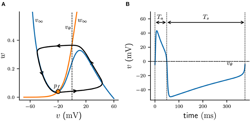
Figure 1. Periodic solution of ML model neuron. (A) Projection of limit cycle onto (v, w)-phase plane with v-nullcline (blue, v_∞) and w-nullcline (orange, w_∞). Unstable fixed point p_f is indicated by an orange dot; firing threshold v_θ is denoted by a dashed line. (B) Corresponding voltage trace v(t) of an action potential.

The two-cell network model is numerically integrated using an adaptive step-size integrator for stiff differential equations implemented with XPPAUT [16] and controlled through the Python packages SciPy [17] and PyXPP [18]. The following mathematical analysis is performed on the equations of a single cell. Unless required for clarity, we will therefore omit the subscripts i, j from here on.

3. Results

3.1. Anti-phase Burst Solutions

Short-term synaptic depression of inhibition in a half-center oscillator acts as a burst termination mechanism [7] and is known to produce n : n anti-phase burst solutions of varying period. Such n : n solutions consist of cells firing bursts of n spikes in alternation. Figure 2D shows the timecourse of a typical 4 : 4 burst. While one cell is firing a burst it provides an inhibitory conductance to the other cell, preventing it from firing.

FIGURE 2

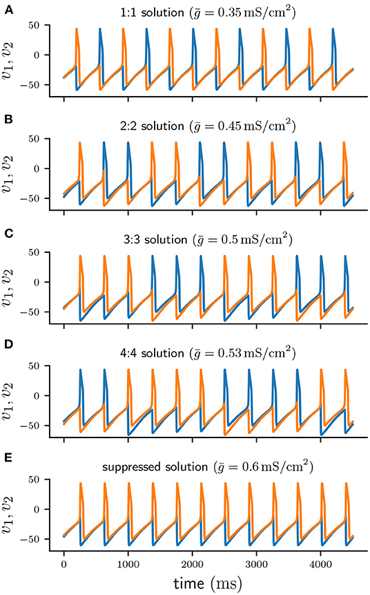
Figure 2. Voltage traces of cell 1 (blue) and cell 2 (orange) of numerically stable solutions. (A–D) 1 : 1, 2 : 2, 3 : 3, and 4 : 4 anti-phase solutions for increasing values of $\overline{g}$. (E) Suppressed solution.

Therefore, at any given moment one cell is spiking while the other is suppressed and does not spike. We will refer to the currently firing cell as “active” and we will call the suppressed cell “silent.” Additionally, we will distinguish between two phases of a n : n solution: We will refer to the time interval when a cell is firing as the “active phase,” and we will call the remaining duration of a cycle, when a cell is not firing, the “silent phase.”

With each action potential of the active cell, short-term depression leads to a decrease of d, and consequently of s. If d depresses faster at spike time than it can recover in the inter-spike-intervals (ISIs), the total synaptic conductance $\overline{g}$s will eventually become sufficiently small to allow for the silent cell to be released [19, 20] and start firing, thus inhibiting the previously active cell. While a cell is silent its depression variable can recover. Once the silent cell becomes active again its synaptic inhibition will be sufficient to terminate the burst of the previously active cell and commence a new cycle. As previously demonstrated by Bose and Booth [6], in a two-cell reciprocally inhibitory network with synaptic depression the coupling strength $\overline{g}$ determines the type of n : n solution. Increasing $\overline{g}$ produces higher n : n burst solutions with more spikes per burst and a longer cycle period. Figure 2 shows numerically stable n : n solutions for varying values of $\overline{g}$. For small values of $\overline{g}$ the network produces anti-phase spiking 1:1 solutions (Figure 2A). As $\overline{g}$ is increased the network generates solutions of increasing n, that is 2 : 2 (Figure 2B), 3 : 3 (Figure 2C), and 4 : 4 (Figure 2D). When $\overline{g}$ is sufficiently large (Figure 2E), one of the cells continuously spikes at its uncoupled period T while the other cell remains fully suppressed. Depending on the initial conditions either of the two cells can become the suppressed cell, which is why the suppressed solution is numerically bistable.

Branches of numerically stable n : n solutions and their associated limit cycle period for varying values of $\overline{g}$ are depicted in Figure 3 (see Supplementary Material 2 for algorithm description). Not only do higher n : n solutions branches require stronger coupling $\overline{g}$, but also within n : n branches the period increases with $\overline{g}$. In line with Bose and Booth [6] we find small overlaps between solution branches indicating numerical bistability, for example such as between the 2 : 2 and 3 : 3 solution branches. Branches of higher n : n burst solutions occur on increasingly smaller intervals of $\overline{g}$, for instance is the $\overline{g}$ interval of the 5 : 5 branch shorter than that of the 4 : 4 branch and so on. The interval between the 5 : 5 branch and the suppressed solution (region between dotted lines in Figure 3) not only contains even higher numerically stable n : n solutions, such as 11 : 11 bursts, but also other non-symmetric n : m solutions as well as irregular, non-periodic solutions. However, the analysis in the following sections will only be concerned with the numerically stable and symmetric n : n solutions.

FIGURE 3

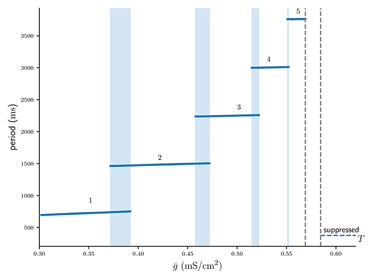
Figure 3. Numerically computed bifurcation diagram of the cycle period of stable n : n solutions for increasing coupling strength $\overline{g}$. Regions of bistability are indicated by light blue vertical stripes. Dashed lines show the interval between the 5 : 5 and the suppressed solution, where higher period n : n solutions occur on increasingly smaller intervals of $\overline{g}$.

3.2. Mathematical Analysis of Two-Cell Network

The goal of the following mathematical analysis is to reduce the complexity of the eight-dimensional system to a more tractable problem. As we will explain, we do this by approximating the full dynamics by a reduced system that describes the evolution of the depression variable d of either of the two cells. We will construct the solution of d in a piecewise manner from one spike to the next, first during the active phase, and then during the silent phase. This construction will require two assumptions about the membrane and synaptic dynamics. The first assumption states that during a burst the active cell fires at its uncoupled period T, which simplifies the construction of the solution of d. The second assumption states that once the inhibitory conductance acting on the silent cell drops below a critical threshold, the cell is immediately released and fires. The second assumption is necessary to predict the release time of the silent cell, which allows us to model the recovery of d during the silent phase. In other words, the second assumption requires that the release of the silent cell from inhibition depends only on the timecourse of the inhibition, and not on the membrane dynamics of the silent cell. The approximate validity of both assumptions can be observed in coupled relaxation-oscillator types of neurons such as the Morris-Lecar model we use, and will be numerically verified below. Both assumptions were first used in Bose and Booth [6] to derive algebraic conditions that guarantee the periodicity of the depression variable for different n : n solutions. However, here we will use these assumptions to construct a Poincaré map of d, which will provide a geometric intuition for the dynamics of the full two-cell network and its dependence on model parameters.

Our first assumption about the model states that the active cell fires at its uncoupled period T, that is, during the active phase of a burst we have ISI = T. Solution profiles in Figure 2 suggest that the ISIs are indeed approximately constant. Numerically computing ISIs for all stable n : n solutions in Figure 3 reveals that ISIs differ by at most 1ms from the intrinsic firing period T ≈ 376 ms. Assuming ISI = T seems reasonable given that inhibition acting on the silent cell decays exponentially on a much shorter timescale τ_κ than the duration of the ISI. Therefore, once the silent cell is released its trajectory quickly approaches the spiking limit cycle. Naturally the above assumption requires a sufficiently small τ_κ, and fails when τ_κ is large. In the Supplementary Material 3 we numerically explore how different values of τ_κ affect the ISIs of the active cell. Finally, assuming ISI = T allows us to ignore the non-linear membrane dynamics during the active phase, and to construct the evolution of the synaptic variables iteratively from spike to spike.

Our second assumption states that the silent cell is released and spikes as soon as the total inhibitory conductance $\overline{g}$s acting on it drops below some threshold value. We call this critical threshold value the “release conductance,” and define it as the value of $\overline{g}$s at the time when the voltage of the silent cell first crosses the firing threshold v_θ, that is when that cell is released and fires its first spike. Recall that when a cell is silent its v- and w-nullclines intersect at a stable fixed point and $\overline{g}$s > g_bif. A sufficient condition for the silent cell to be released is therefore $\overline{g}$s < g_bif. However, depending on the topology of the stable manifold, the (v, w)-trajectory of the silent cell can escape the stable fixed point and allow the cell to produce a spike for $\overline{g}$s > g_bif. In this case the value of the release conductance depends on the type of n : n solution and the coupling strength $\overline{g}$. For any stable n : n solution in Figure 3 we can compute an associated release conductance numerically by recording the value of $\overline{g}$s at the time of the first spike of the silent cell. Such values of the release conductance are shown in Figure 4A, and the graph suggests that as n increases, the value of the release conductance converges to some constant conductance value g^⋆ ≈ 0.0068 mS/cm². Here g^⋆ is the value of $\overline{g}$s at the end of a cycle of a suppressed solution, just before the active cell spikes. Using g^⋆ as a constant approximation for the release conductance will allow us to formulate a scalar condition that predicts the release time of the silent cell. Moreover, using g^⋆ is convenient because its exact value can be derived explicitly, as will be shown in the following section.

FIGURE 4

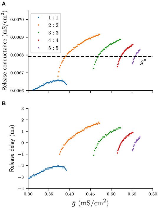
Figure 4. Numerically computed values of the release conductance (A) and release delay (B) for various n : n solutions and values $\overline{g}$. The dashed line indicates the analytical approximation of the release conductance by g^⋆.

Assuming a constant release conductance for all n : n solutions will naturally introduce some error in the prediction of the release time of the silent cell. We can compute that error for any associated solution in Figure 4A by calculating the time interval between the first spike of the silent cell and the time when $\overline{g}$s first crosses g^⋆. We will call this time interval the “release delay.” Figure 4B shows the numerically computed graph of such release delays. For n > 1 the absolute delays are smaller than 2 ms. Therefore, using

$\begin{array}{ll}\overline{g}s=g^{\star }& (7)\end{array}$

as a constant release condition for all n : n solutions allows us to accurately predict the timing of the release of the silent cell. And to simplify the terminology, from now on we will refer to Equation (7) simply as the “release condition.”

In summary: We assume that the release condition is sufficient to predict when the silent cell is released. Due to the symmetry of n : n solutions the release occurs at exactly half the period of the full cycle. The release time therefore uniquely determines the type of n : n solution. Furthermore, computation of the release time does not depend on the membrane nor the synaptic dynamics of the silent cell. Instead, the solution of the synaptic variable s of the active cell is sufficient to predict when $\overline{g}$s = g^⋆ is satisfied. Finally, the value of s at each spike time is determined by the evolution of the depression variable d of the active cell. Constructing a solution of d during the active phase of either cell will therefore uniquely determine the solution of the full eight-dimensional network. However, finding the solution d requires us to know the initial value d(0) at the start of a cycle at t = 0. In the next section we will construct a scalar return map that tracks these initial values d(0) from cycle to cycle of stable n : n solutions.

3.3. Construction of the Scalar Poincaré Map

In this section we construct the scalar Poincaré map ${\Pi }_n:d^{\star }\mapsto d^{\star }$. Here the discrete variable d^⋆ tracks the values of the continuous depression variable d at the beginning of each n : n burst. The map Π_n therefore describes the evolution of d, of either of the two cells, from the beginning of one cycle to the beginning of the next cycle. To simplify the map construction we will assume that an active cell fires exactly n times before it becomes silent. We will construct Π_n by evolving d first during the active phase and then during the silent phase of the n : n limit cycle. The terms “active” and “silent” phases will be defined in terms of the state of the depression variable. During the active phase the depression variable of the active cell both decays and recovers, while during the silent phase it only recovers. First, let us give explicit definitions of the active and silent phases of a burst. A schematic illustration of both phases is given in Figure 5.

FIGURE 5

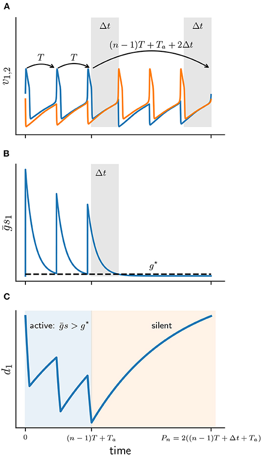
Figure 5. Schematic diagram of the active and silent phases for a 3 : 3 solution. (A) Membrane potentials of cell 1 (v₁ blue) and cell 2 (v₂ orange). Gray patches depict Δt intervals. (B) Total synaptic conductance of cell 1 ($\overline{g}$s₁) as it crosses the release conductance g^⋆. (C) Solution d₁(t) of depression variable of cell 1, during active (blue) and silent phases (orange).

Suppose that at t = 0 cell 1 becomes active with some initial d(0). Cell 1 then fires n spikes at the uncoupled period T = T_a + T_s. Let s(t) and d(t) be the corresponding solutions of the synaptic and depression variables of cell 1. After n spikes the total conductance $\overline{g}$s(t) acting on the silent cell 2 has decayed sufficiently to satisfy the release condition (Equation 7). That is at some time t = (n − 1)T + T_a + Δt, where Δt < T_s will be determined below, we have $\overline{g}$s(t) = g^⋆ [6]. Cell 2 is then released and prevents cell 1 from further spiking. Once released, cell 2 also fires n spikes until cell 1 becomes active once again. Let P_n denote the full cycle period of a n : n solution:

$\begin{array}{ll}{P}_n=2\left[(n-1)T+T_a+\Delta t\right].& (8)\end{array}$

We can now define the active and silent phases of cell 1 explicitly. The active phase of a burst is the interval that lasts from the first spike time up until the beginning of the silent phase of the last spike, that is for time 0 < t < (n − 1)T + T_a. During the active phase of cell 1, the silent cell 2 is inhibited sufficiently strong to prevent it from firing, hence $\overline{g}$s > g^⋆. The silent phase of cell 1 is the remaining duration of the cycle when the cell is not firing, that is for (n − 1)T + T_a < t < P_n. The silent phase lasts for (n − 1)T + T_a + 2Δt.

Note that only the silent phase depends on Δt, which will play a central role in the construction of Π_n. From Equation (8) Δt can be computed as

$\begin{array}{ll}\Delta t=\frac{1}{2}{P}_n-(n-1)T-T_a.& (9)\end{array}$

We can use Equation (9) and the numerically computed bifurcation diagram of the period for stable n : n solutions in Figure 3 to obtain the graph of Δt as a function of $\overline{g}$ (Figure 6). Each continuous branch of Δt is monotonically increasing and corresponds to a n : n burst: Stronger coupling $\overline{g}$ increases the total synaptic conductance $\overline{g}$s that acts on the silent cell, thus delaying its release. It is easy to see that for any n-branch we have Δt < T_s: Once Δt crosses T_s, the active cell can “squeeze in" an additional spike and the solutions bifurcate into a (n + 1) : (n + 1) burst.

FIGURE 6

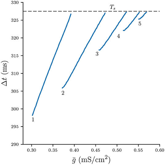
Figure 6. Numerically computed bifurcation diagram of Δt for varying $\overline{g}$. Each continuous branch is associated with a stable n : n burst solution. Increasing $\overline{g}$ increases Δt until the solutions bifurcate at Δt ≈ T_s.

Distinguishing between the active and silent phases of a n : n cycle allows us to describe the dynamics of the depression variable d explicitly for each phase. As can be seen from Figure 5C, during the active phase d depresses when v > v_θ and recovers when v < v_θ. In contrast, during the silent phase d only recovers and does not depress. Given the initial d^⋆ = d(0) at the beginning of the cycle and the number of spikes in the active phase n, we can now construct the burst map Π_n. The map

$\begin{array}{ll}{\Pi }_n(d^{\star })=Q_n\left[F_n(d^{\star })\right]& (10)\end{array}$

is a composition of two maps. Map

$\begin{array}{ll}{F}_n:d^{\star }\mapsto \Delta t& (11)\end{array}$

models the evolution of d in the active phase. F_n takes an initial value d^⋆ and calculates Δt. Map

$\begin{array}{ll}{Q}_n:\Delta t\mapsto d^{\star }& (12)\end{array}$

models the recovery of d in the silent phase. Given some Δt map Q_n computes d^⋆ at the start of the next cycle.

Our aim in the following analysis is to elucidate the properties of Π_n and to understand the structure of its parameter space by exploring how the stable and unstable fixed points of Π_n are created. To that effect it will be useful to include not only positive, but also negative values of d^⋆ to the domain of Π_n. But it is important to add that values d^⋆ < 0 are biologically impossible as the depression variable models a finite pool of neurotransmitters, and therefore must be positive. Because Π_n maps first from d^⋆ to Δt, and then back to d^⋆, we will also consider negative values of Δt, interpreting them as n : n solutions with partially overlapping bursts. As will become evident, Δt < 0 is only a formal violation of the biological realism of the map Π_n, as numerically stable n : n solutions of the full system of ODEs only exist for Δt > 0.

We start the construction of Π_n by first considering the active phase and building the map F_n. At each spike time t_k where d(t_k) = d_k, variable d decays first for the duration of T_a, as described by the solution to Equation (5). At t = t_k + T_a we have

$\begin{array}{ll}d(t_k+T_a)=d_k{e}^{-T_a/{\tau }_b}.& (13)\end{array}$

The depression variable then recovers for T_s until t_k+1, where for 0 < t < T_s:

$\begin{array}{ll}d(t_{k+1})=1-(1-d_k{e}^{-T_a/{\tau }_b})e^{-t/{\tau }_a}.& (14)\end{array}$

By substituting t = T_s we can build a linear map that models the depression of d from spike time t_k to the subsequent spike time t_k+1 during the active phase:

$\begin{array}{ll}{d}_{k+1}=\text{λ}\rho d_k+(1-\rho ),& (15)\end{array}$

where to keep the notation simple we let

$\begin{array}{ll}\text{λ}:=exp(-T_a/{\tau }_b),& (16)\end{array}$

$\begin{array}{ll}\rho :=exp(-T_s/{\tau }_a).& (17)\end{array}$

Given constant T_a and T_s, the derived parameter λ determines how much the synapses depresses when v > v_θ, while ρ determines how much it recovers when v < v_θ. Since 0 < λ, ρ < 1, the map in Equation (15) is increasing and contracting, with a fixed point at

$\begin{array}{ll}{d}_s=\frac{1-\rho }{1-\text{λ}\rho },& (18)\end{array}$

where 0 < d_s < 1. The value d_s is the maximum depression value that can be observed in the suppressed solution where the active cell fires at its uncoupled period T (see Figure 2E). Using the release condition in Equation (7) allows us to derive the value of the minimum coupling strength that will produce the full suppressed solution, denoted as $\overline{g}$_s. Solving Equation (7) for s(t) with t = T_s and setting the initial value s(0) = d_sλ then gives us the aforementioned approximation of the release conductance g^⋆:

$\begin{array}{ll}{\overline{g}}_s{d}_s\text{λ}{e}^{-T_s/{\tau }_{\kappa }}=g^{\star }\approx 0.0068mS/c{m}^2.& (19)\end{array}$

By substituting the definition of d_s in Equation (18) and rearranging, we can also write $\overline{g}$_s as a function of λ and ρ:

$\begin{array}{ll}{\overline{g}}_s(\text{λ},\rho )=\frac{1/\text{λ}-\rho }{1-\rho }{e}^{T_s/{\tau }_{\kappa }}{g}^{\star }.& (20)\end{array}$

Note that the above dependence of $\overline{g}$_s on λ is linear and monotonically decreasing. Increasing λ reduces the strength of the depression of the active cell. This in turn allows the active cell to fully suppress the silent cell at smaller values of $\overline{g}$.

Solving Equation (15) gives us the linear map δ_n, that for some initial d^⋆ computes the depression at the nth spike time, that is d(t_n):

$\begin{array}{ll}{\delta }_n(d^{\star })={(\text{λ}\rho )}^{n-1}{d}^{\star }+(1-\rho ){\displaystyle \sum _{i=0}^{n-2}}{(\text{λ}\rho )}^i.& (21)\end{array}$

Since λ < 1, function δ_n is a linearly increasing function of d^⋆ with a fixed point at d_s for all n. Having identified d after n spikes, we can now use the release condition $\overline{g}$s = g^⋆ (Equation 7) to find Δt. At the last (nth) spike of the active phase at time t_n = (n − 1)T the synapse variable s is set to the respective value of $d(t_n)={\delta }_n(d^{\star })$, and mirrors the value of d for the duration of T_a. At the end of the active phase at time t_n + T_a variable d has decayed to ${\delta }_n(d^{\star })\text{λ}$, therefore

$\begin{array}{ll}s(t_n+T_a)={\delta }_n(d^{\star })\text{λ}.& (22)\end{array}$

Finally s decays exponentially for Δt < T_s. Solving (Equation 6) with initial condition $s(0)={\delta }_n(d^{\star })\text{λ}$ yields:

$\begin{array}{ll}s(\Delta t)={\delta }_n(d^{\star })\text{λ}{e}^{-\Delta t/{\tau }_{\kappa }}.& (23)\end{array}$

Substituting s(Δt) into s of the release condition (Equation 7) gives then

$\begin{array}{ll}\overline{g}{\delta }_n(d^{\star })\text{λ}{e}^{-\Delta t/{\tau }_{\kappa }}=g^{\star }.& (24)\end{array}$

Our assumption of the release condition guarantees that the silent cell 2 spikes and becomes active when $\overline{g}$s − g^⋆ crosses zero. Solving (Equation 24) for Δt allows us to compute Δt as a function of d^⋆, which defines the map F_n:

$\begin{array}{ll}{F}_n(d^{\star }):={\tau }_{\kappa }ln\left(\frac{\overline{g}}{g^{\star }}\text{λ}{\delta }_n(d^{\star })\right)=\Delta t.& (25)\end{array}$

Figure 7A shows F_n for various n, which is a strict monotonically increasing function of d^⋆ as well as $\overline{g}$. Larger values of d^⋆ and $\overline{g}$, respectively, cause stronger inhibition of the silent cell, and therefore prolong its release time and the associated Δt. Map F_n is defined on $d^{\star }>d_a$, where d_a is a vertical asymptote found by solving ${\delta }_n(d^{\star })=0$ in Equation (21) for d^⋆, which yields

$\begin{array}{ll}{d}_a(n)=-\frac{(1-\rho ){\displaystyle {\sum }_{i=0}^{n-2}}{(\text{λ}\rho )}^i}{{(\text{λ}\rho )}^{n-1}}\le 0.& (26)\end{array}$

We now turn to the construction of map Q_n, which describes the recovery of the depression variable during the silent phase. As we have identified earlier, the recovery of d in the silent phase of a n : n solution starts at time t_n + T_a and lasts for the duration of (n − 1)T + T_a + 2Δt. Substituting that duration into the solution of d (Equation 5) with the initial condition $d(0)={\delta }_n(d^{\star })\text{λ}$ yields the map Q_n:

$\begin{array}{ll}{Q}_n(\Delta t):=1-\left[1-{\delta }_n(d^{\star })\text{λ}\right]e^{-\left[(n-1)T+T_a+2\Delta t\right]/{\tau }_a}.& (27)\end{array}$

We can find ${\delta }_n(d^{\star })$, i.e., the value of d at the nth spike time, by rearranging the release condition in Equation (24):

$\begin{array}{ll}{\delta }_n(d^{\star })=\frac{1}{\overline{g}\text{λ}}{g}^{\star }{e}^{\Delta t/{\tau }_{\kappa }}.& (28)\end{array}$

Map Q_n is shown in Figure 7B for various values n. Note that Q_n is monotonically increasing as larger values Δt imply a longer recovery time, and hence Q_n grows without bound. All curves Q_n intersect at some $\Delta t={\tau }_{\kappa }ln\left[\overline{g}/g^{\star }\right]$ where

$\begin{array}{ll}{Q}_n\left[{\tau }_{\kappa }ln\left(\frac{\overline{g}}{g^{\star }}\right)\right]=1.& (29)\end{array}$

As we will show in the next section, all fixed points of the full map Π_n occur for d^⋆ < 1. We will therefore restrict the domain of Q_n to $(-\infty ,{\tau }_{\kappa }ln\left[\overline{g}/(g^{\star })\right])$ and the codomain to (−∞, 1). Additionally, while values Δt > T will be helpful in exploring the geometry of Π_n, recall from Figure 6 that in the flow system n : n solutions bifurcate into (n + 1) : (n + 1) solutions exactly when Δt = T_s, and we will address this concern in the last part of our map analysis.

FIGURE 7

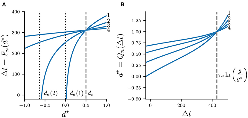
Figure 7. Maps F_n (A) and Q_n (B) for $\overline{g}$ = 0.5 mS/cm² and n = 1, 2, 3, 4. Curves F_n intersect at $d^{\star }=d_s$ which is indicated by a dashed vertical line. Curves Q_n intersect at $\Delta t={\tau }_{\kappa }ln\left(\overline{g}/g^{\star }\right)$.

Having found F_n and Q_n, we can now construct the full map ${\Pi }_n(d^{\star })=Q_n\left[F_n(d^{\star })\right]$:

$\begin{array}{ll}{\Pi }_n(d^{\star })=1-\left[1-{\delta }_n(d^{\star })\text{λ}\right]{\left[\frac{\overline{g}}{g^{\star }}{\delta }_n(d^{\star })\text{λ}\right]}^{-\tau }{e}^{-\left[(n-1)T+T_a\right]/{\tau }_a},& (30)\end{array}$

where we substituted τ = 2τ_k/τ_a. Recall that ${\delta }_n(d^{\star })$ and g^⋆ are obtained from Equations (21) and (19), respectively. Since d is the slowest variable of the system and τ_a ≫ τ_κ, we will also assume τ < 1. Figure 8A depicts Π_n for various n. Intersections of Π_n with the diagonal are fixed points of the map. Figure 8B shows Π₂ with n = 2. Varying the synaptic strength $\overline{g}$ moves the curves Π_n up and down the $(d^{\star },{\Pi }_n)$-plane. For $\overline{g}$ < 0.0015 mS/cm² map Π₂ has no fixed points. As $\overline{g}$ is increased to $\overline{g}$ ≈ 0.0015 mS/cm², curve Π₂ coalesces with the diagonal tangentially. When $\overline{g}$ > 0.0015 mS/cm², a pair of fixed points emerge, one stable and one unstable fixed point, indicating the occurrence of a fold bifurcation of maps.

FIGURE 8

Figure 8. Map ${\Pi }_n:d^{\star }\mapsto d^{\star }$. (A) Π_n for n = 1, 2, 3, 4 at $\overline{g}$ = 0.5 mS/cm². (B) Π₂ with n = 2 for various $\overline{g}$. The identity function is illustrated by a diagonal line.

Π_n is monotonically increasing with respect to $\overline{g}$ and also d^⋆:

$\begin{array}{ll}\frac{d{\Pi }_n}{d\overline{g}}>0,& (31)\end{array}$

$\begin{array}{ll}\frac{d{\Pi }_n}{d{d}^{\star }}>0.& (32)\end{array}$

The monotonicity of Π_n w.r.t. $\overline{g}$ is evident from Equation (30), while the monotonicity w.r.t. d^⋆ follows from the monotonicity of both Q_n and F_n. In the following sections we will heavily rely on this monotonicity property of Π_n. Just as F_n, curves Π_n spawn at the asymptote d_a (Equation 26), and because

$\begin{array}{ll}{\displaystyle \underset{\overline{g}\to \infty }{lim}}{\Pi }_n=1\text{ for all }n,& (33)\end{array}$

fixed points of Π_n lie in (d_a, 1).

3.4. Existence and Stability of Fixed Points

We introduce the fixed point notation $d_f^{\star }$ with ${\Pi }_n(d_f^{\star })=d_f^{\star }$. The existence of fixed points $d_f^{\star }$ for $\overline{g}$ sufficiently large can be shown from the strict monotonicity of Π_n with respect to $\overline{g}$ and d^⋆ (Equations 32, 31), as well as the fact that the slope of Π_n is monotonically decreasing,

$\begin{array}{ll}{\left(\frac{\text{d}}{\text{d}{d}^{\star }}\right)}^2{\Pi }_n<0.& (34)\end{array}$

In the limit $d^{\star }\to d_a$ the value of Π_n decreases without bound for any $\overline{g}$ > 0. In the limit $\overline{g}$ → 0, Π_n also decreases without bound, but as $\overline{g}$ → ∞ values of Π_n approach 1. It follows from Equation (31) and the intermediate value theorem that for some $\overline{g}$ large enough Π_n intersects the diagonal. Moreover, because Π_n and its slope are monotonic with respect to d^⋆, there exists some critical fixed point $(d_b^{\star },{\overline{g}}_b)$ where Π_n aligns with the diagonal tangentially with

$\begin{array}{ll}{\Pi }_n(d_b^{\star },{\overline{g}}_b)=d_b^{\star },& (35)\end{array}$

$\begin{array}{ll}\frac{d}{d{d}^{\star }}{\Pi }_n({d^{\star }}_b,{\overline{g}}_b)=1.& (36)\end{array}$

3.5. Fold Bifurcations of Maps

Fixed points of Π_n satisfy the fixed point equation

$\begin{array}{ll}{\Phi }_n(d^{\star },\overline{g}):={\Pi }_n(d^{\star },\overline{g})-d^{\star }=0.& (37)\end{array}$

As we have already shown, for $\overline{g}$ > $\overline{g}$_b(n) solutions to Equation (37) exist in pairs of stable and unstable fixed points. Solving (Equation 37) explicitly for d^⋆ is not trivial, but solving for $\overline{g}$ is straightforward and given by $\overline{g}=G_n(d^{\star })$, where

$\begin{array}{ll}{G}_n(d^{\star }):=\frac{g^{\star }}{{\delta }_n(d^{\star })\text{λ}}{\left(\frac{\left[1-\text{λ}{\delta }_n(d^{\star })\right]}{1-d^{\star }}{e}^{-\left[(n-1)T+T_a\right]/{\tau }_a}\right)}^{1/\tau }& (38)\end{array}$

is defined for d^⋆ < 1 and ${\delta }_n(d^{\star })>0$. Plotting d^⋆ against $\overline{g}$ gives the fixed point curves, which are shown in Figure 9A. Note the typical quadratic shape of a fold bifurcation of maps. It is also evident that the fold bifurcations occur for increasingly smaller $\overline{g}$ as n is increased. Moreover, the graph suggests that for n > 1 unstable fixed points have negative values of d^⋆.

FIGURE 9

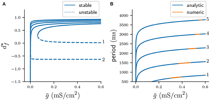
Figure 9. (A) Fold bifurcation diagrams of stable (continuous curves) and unstable (dotted curves) fixed points of Π_n for varying n. (B) Cycle periods computed from stable fixed points of Π_n (blue), and the corresponding periods from stable n : n solutions acquired via numerical integration of the system of ODEs (orange).

Equation (38) also allows us to find the critical fixed point connected with the fold bifurcation, namely $\left[d_b^{\star }(n),{\overline{g}}_b(n)\right]$, which is the global minimum of $G_n(d_f^{\star })$:

$\begin{array}{ll}{d}_b^{\star }(n)=argmin{G}_n(d_f^{\star }),& (39)\end{array}$

$\begin{array}{ll}{\overline{g}}_b(n)=min{G}_n(d_f^{\star }).& (40)\end{array}$

Function G_n is strictly monotonic on the respective intervals of $d_f^{\star }$ that correspond to the stable and unstable fixed points, that is

$\begin{array}{ll}\frac{d{G}_n}{d{d}_f^{\star }}>0,\text{for }{d}_f^{\star }>d_b^{\star }(n)\text{ stable},& (41)\end{array}$

$\begin{array}{ll}\frac{d{G}_n}{d{d}_f^{\star }}<0,\text{for }{d}_f^{\star }<d_b^{\star }(n)\text{ unstable},& (42)\end{array}$

which allows us to express the stable and unstable fixed points as the inverse of G_n on their respective intervals of $d_f^{\star }$. Because we are primarily interested in the stable fixed points $d_f^{\star }>d_b^{\star }(n)$, we define the stable fixed point function $d_f^{\star }={\varphi }_n(\overline{g})$ as

$\begin{array}{ll}{\varphi }_n(\overline{g}):=G_n^{-1}(\overline{g}).& (43)\end{array}$

Function ϕ_n($\overline{g}$) is also monotonic, and is therefore straightforward to compute numerically. We use the Python package Pynverse [21] for that purpose.

Having found the stable fixed points $d_f^{\star }$ as a function of $\overline{g}$, we can now compute the associated cycle period. Recall that the period is given by Equation (8), which can be written as a function of $\overline{g}$:

$\begin{array}{ll}{P}_n(\overline{g})=2((n-1)T+T_a+F_n[{\displaystyle \underset{d_f^{\star }}{{\displaystyle \underbrace{{\varphi }_n(\overline{g})}}}},\overline{g}]),& (44)\end{array}$

where map F_n (Equation 25) calculates Δt given a stable fixed point $d_f^{\star }={\varphi }_n(\overline{g})$. Figure 9B shows the period P_n($\overline{g}$) computed from Equation (44) versus the cycle period of stable n : n solutions, computed from numerically integrating the full system of ODEs. The overlap between blue and orange curves suggests that stable fixed points of Π_n accurately predict the cycle period of stable solutions of the flow system.

It is evident from Figure 9A that ϕ_n is strictly increasing with $\overline{g}$. This property follows directly from the quadratic normal form of the fold bifurcation, but can also be shown using implicit differentiation and the fixed point equation Φ_n[ϕ_n($\overline{g}$), $\overline{g}$] = 0 in Equation (37). For $d_f^{\star }={\varphi }_n(\overline{g})>d_b(n)$ we get:

$\begin{array}{ll}\frac{d{\varphi }_n}{d\overline{g}}=-\frac{\partial {\Phi }_n/\partial \overline{g}}{\partial {\Phi }_n/\partial d^{\star }}=\frac{\partial {\Pi }_n/\partial \overline{g}}{1-\partial {\Pi }_n/\partial d^{\star }}>0.& (45)\end{array}$

The inequality follows from ∂Π_n/∂$\overline{g}$ > 0 and the fact that $\partial {\Pi }_n/\partial d^{\star }<1$ for $d^{\star }>d_b(n)$. Equation (45) allows us to explain why the period P_n increases with $\overline{g}$, as seen in Figure 9B. Differentiating P_n gives:

$\begin{array}{ll}\frac{d{P}_n}{d\overline{g}}=2▽F_n(d_f^{\star },\overline{g})·\left[\begin{array}{c}\partial {\varphi }_n/\partial \overline{g}\\ 1\end{array}\right]>0,& (46)\end{array}$

where the partial derivatives of $F_n(d_f^{\star },\overline{g})$ are:

$\begin{array}{ll}\frac{\partial F_n}{\partial d_f^{\star }}={\tau }_{\kappa }\frac{{(\text{λ}\rho )}^{n-1}}{{\delta }_n(d_f^{\star })}>0,& (47)\end{array}$

$\begin{array}{ll}\frac{\partial F_n}{\partial \overline{g}}=\frac{{\tau }_{\kappa }}{\overline{g}}>0.& (48)\end{array}$

Equation (46) and (47) have an intuitive biological interpretation: Increasing the coupling strength between the neurons leads to overall stronger inhibition of the silent cell, which delays its release and leads to a longer cycle period. The latter allows more time for the synapse to depress in the active phase and recover in the silent phase, resulting in overall larger values of $d_f^{\star }$, that is weaker depression at the burst onset.

While fixed points of our Poincaré map predict the cycle period of the flow system excellently, its construction relies on the strong assumption that the active phase contains exactly n spikes. As is evident from Figure 9B this assumption is clearly violated in the flow system, as stable n : n bursts exists only on certain parameter intervals of $\overline{g}$. The multi-stability of fixed points of maps Π_n in Figure 9B does therefore not imply a similar multi-stability of the flow system. In the last sub-section we will analyze the mechanisms that guide how the stable n : n are created and destroyed, and use our previous analysis to derive the corresponding parameter intervals of $\overline{g}$ where such solutions exist.

3.6. Stable Solution Branch Borders

Let ${\overline{g}}_{{L}}(n)$ and ${\overline{g}}_{{R}}(n)$ denote the left and right parameter borders on $\overline{g}$ where stable n : n solutions exist. That is, as $\overline{g}$ is increased stable n : n solutions are created at ${\overline{g}}_{{L}}(n)$ and destroyed at ${\overline{g}}_{{R}}(n)$. When $\overline{g}$ is reduced beyond ${\overline{g}}_{{L}}(n)$, n : n solutions bifurcate into (n − 1) : (n − 1) solutions, while when $\overline{g}$ is increased beyond ${\overline{g}}_{{R}}(n)$, n : n solutions bifurcate into (n + 1) : (n + 1) solutions. Let us briefly recap our observations regarding ${\overline{g}}_{{L}}(n)$ and ${\overline{g}}_{{R}}(n)$ from the numerical bifurcation diagram in Figure 9B. For n > 1 there are the following relations:

$\begin{array}{ll}{\overline{g}}_{{L}}(n)<{\overline{g}}_{{R}}(n),& (49)\end{array}$

$\begin{array}{ll}{\overline{g}}_{{L}}(n)<{\overline{g}}_{{R}}(n+1)\text{ and }{\overline{g}}_{{R}}(n)<{\overline{g}}_{{L}}(n+1),& (50)\end{array}$

$\begin{array}{ll}{\overline{g}}_{{L}}(n)<{\overline{g}}_{{R}}(n)& (51)\end{array}$

$\begin{array}{ll}{\overline{g}}_{{L}}(n)<{\overline{g}}_{{L}}(n+1)\text{ and }{\overline{g}}_{{R}}(n)<{\overline{g}}_{{R}}(n+1)& (52)\end{array}$

Equations (49, 50) are self-explanatory. Equation (51) formally describes occurrence of co-existence between stable n : n and (n + 1) : (n + 1) solutions. Equation (52) implies that the parameter interval on $\overline{g}$ of n : n solutions decreases with n, in other words, bursts with more spikes occur on increasingly smaller intervals of the coupling strength. All of the above relations are reminiscent of the bifurcation scenario of type period increment with co-existent attractors, first described for piecewise-linear scalar maps with a single discontinuity by Avrutin and colleagues [e.g., see 22–24]. While our maps Π_n are fully continuous, the above observation suggests that a different piecewise-linear scalar map that captures such period increment dynamics of the full system might exist. We will explore what such a map might look like in the discussion.

Let us now find algebraic equations that will allow us to calculate the critical parameters ${\overline{g}}_{{L}}(n)$ and ${\overline{g}}_{{R}}(n)$ associated with the left and right n : n branch borders. Recall that the period P_n derived from the fixed points of Π_n is an increasing function of $\overline{g}$ (Equation 46). That is, as the coupling strength increases, it takes longer for the total synaptic conductance to fall below the value of the release conductance, which delays the release of the silent cell, and Δt becomes larger. When Δt > T_s, the active cell can produce another spike and the solution bifurcates into a (n + 1) : (n + 1) solution. Note, however, that at ${\overline{g}}_{{L}}(n)$ the bifurcation into a (n − 1) : (n − 1) does not occur at Δt = 0. Here the mechanism is different: A sufficient reduction of $\overline{g}$ causes the total synaptic conductance to drop below the release conductance in the previous ISI, which allows the silent cell to be released one spike earlier.

Using the above reasoning we can now formulate the conditions for both bifurcations at ${\overline{g}}_{{L}}(n)$ and ${\overline{g}}_{{R}}(n)$. As in the previous sections, we will only restrict ourselves to the analysis of the stable fixed points given implicitly by $d_f^{\star }={\varphi }_n(\overline{g})$ (Equation 43). At the right bifurcation border ${\overline{g}}_{{R}}(n)$ we have Δt = T_s, and after substituting our F_n map (Equation 25) this translates into

$\begin{array}{ll}{\overline{g}}_{{L}}(n+1)<{\overline{g}}_{{R}}(n)& (53)\end{array}$

which lets us define a function

$\begin{array}{ll}{\overline{g}}_{{R}}(n+1)-{\overline{g}}_{{L}}(n+1)<{\overline{g}}_{{R}}(n)-{\overline{g}}_{{L}}(n)& (54)\end{array}$

whose root is the desired right bifurcation border ${\overline{g}}_{{R}}(n)$. In case of the left bifurcation border at ${\overline{g}}_{{L}}(n)$, the release condition is satisfied just before the active cell has produced its nth spike, where total synaptic conductance is given by

$\begin{array}{ll}\overline{g}{\delta }_{n-1}\left[{\varphi }_n(\overline{g})\right]\text{λ}{e}^{-T_s/{\tau }_{\kappa }}=g^{\star },& (55)\end{array}$

which can be rewritten as a function

$\begin{array}{ll}{{L}}_n(\overline{g}):=\overline{g}{\delta }_{n-1}\left[{\varphi }_n(\overline{g})\right]\text{λ}{e}^{-T_s/{\tau }_{\kappa }}-g^{\star },& (56)\end{array}$

whose root is ${\overline{g}}_{{L}}(n)$. Both ${{R}}_n$ and ${{L}}_n$ are increasing with respect to $\overline{g}$, which makes finding their roots numerically straightforward.

Figure 10 shows the period P_n($\overline{g}$) as predicted by the fixed points of Π_n (Equation 44) plotted on their respective intervals $\overline{g}\in \left[{\overline{g}}_{{L}}(n),{\overline{g}}_{{R}}(n)\right]$ (blue), as well as the cycle period acquired from numerical integration of the full system of ODEs (orange). Here $g_{{L}}(n)$ and ${\overline{g}}_{{R}}(n)$ were computed from Equations (56) and (54), respectively. Note that the width of n : n branches decreases with n, which confirms the inequality in Equation (52). That is, bursts with more spikes occur on increasingly smaller intervals of $\overline{g}$, which can be interpreted as a lost of robustness with respect to the coupling strength of long-cyclic solutions. We also note the occurrence of bistability between pairs of n : n and (n + 1) : (n + 1) branches, which also confirms our initial observation in Equation (51). As previously observed in Figure 9B our maps prediction of the cycle period is accurate. However, the mismatch in the left and right branch borders is significant. This mismatch might be due to the millisecond release delay error (Figure 4B) induced by our assumption of a constant release conductance for all n : n solutions (see Equation 7). Another explanation for the border mismatch could be that our assumptions on the time scales of (v, w) vs s- and d-dynamics do not hold near the stability borders, and that they can only be captured by more complex approximations. Nevertheless, our map allows approximate extrapolation of the cycle period and the respective bifurcation borders where numerical integration of the ODEs would require a very small time step.

FIGURE 10

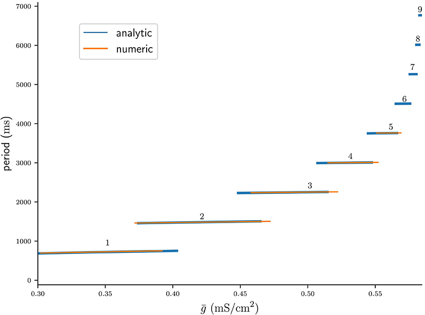
Figure 10. Bifurcation diagram of the period of stable n : n solutions computed analytically from fixed points of Π_n, plotted on the respective intervals of $\overline{g}\in \left[{\overline{g}}_{{L}}(n),{\overline{g}}_{{R}}(n)\right]$ (blue), and computed from numerical integrations of the ODEs (orange).

4. Discussion

Synaptic depression of inhibition is believed to play an important role in the generation of rhythmic activity involved in many motor rhythms such as in leech swimming [25] and leech heart beat [26], and in the lobster pyloric system [1, 2]. In inhibitory half-center CPGs, such as believed to be found in the struggling network of Xenopus tapdoles, synaptic depression can act as a burst termination mechanism, enabling the alternation of bursting between the two sides of the CPG [11]. Modeling can shed light on the underlying mathematical principles that enable the generation of such anti-phase bursts, and help identify the components that control this rhythm allowing it to switch between different patterns.

To study the mechanisms of burst generation in half-center CPGs we have analyzed a neuronal model network that consists of a pair of inhibitory neurons that undergo a frequency dependent synaptic depression. When the strength of synaptic inhibition between the neurons is varied, such a simple network can display a range of different n : n burst patterns. Using the timescale disparity between neuronal and synaptic dynamics, we have reduced the network model of eight ODEs to a scalar first return map Π_n of the slow depression variable d. This map Π_n is a composition of two maps, F_n and Q_n, that model the evolution of the depression during the active and silent phases of n : n solutions respectively. Both F_n and Q_n maps are constructed by using the dynamics of a single uncoupled neuron. Fixed points of Π_n are created in pairs through a fold bifurcation of maps, where the stable fixed point correspond to stable n : n burst solutions of the full two-cell system of ODEs. The results from our one-dimensional map match excellently with numerical simulation of the full network. Our results are also in line with Brown's [7] rhythmogenesis hypothesis, namely that synaptic depression of inhibition is a mechanism by which anti-phase bursting may arise.

We have studied n : n solutions assuming that the synaptic coupling $\overline{g}$ between the two cells is symmetrical. However, Bose and Booth [6] have shown that asymmetrical coupling ($\overline{g}$₁, $\overline{g}$₂) can result in network solutions of type m : n, where one cell fires m spikes, while the other n spikes. It is conceivable that our map construction can be extended to also capture such m : n solutions. Remember, in the case of symmetrical coupling with n : n solutions, the timecourse of the depression variables d₁ and d₂ were in anti-phase, and it was therefore sufficient to track only one of the two variables. To capture the full network dynamics in case of asymmetrical coupling one would also have to account for burst patterns of type m : n, where the solutions of the depression variables d₁ and d₂ are not simply time-shifted versions of each other. To do that, one could track the state of both variables by constructing a two-dimensional Poincaré map Π(d₁, d₂). While geometrical interpretation of two-dimensional maps remains challenging, there exist a number of recent studies which have employed novel geometrical analysis methods to understand the dynamics of two-dimensional maps of small neuronal networks [27–29]. Generally speaking, our map construction approach is applicable to any small network, even with more than two neurons. As long as the network dynamics occur on separable timescales the main challenges to the map construction lie in identifying the slowest variables, and finding an appropriate, simplified description of their respective timecourses. In theory, the reduction approach can be also applied to neuronal systems with more than two timescales [e.g., see 30].

In tadpoles, struggling is believed to be initiated by an increase in the firing frequency of reciprocally inhibitory commisural interneurons, which has been hypothesized to lead to stronger synaptic depression of inhibition and result in the iconic anti-phase bursting [11]. It would therefore be interesting to study how varying the cell intrinsic firing period T could affect the network rhythm. While we have laid out the framework to perform such an investigation, due to the choice of neural model we have avoided varying T. Recall that T is a derived parameter in the Morris and Lecar [12] model, and can therefore not be varied in isolation of other model parameters. This makes verifying any analytical results from our map analysis via numerical integration of the ODEs difficult. A more abstract model such as the quadratic integrate-and-fire model [31] allows varying T independently of other model parameters, and could be more fitting for such an investigation.

Our simulations of the network showed that n : n solutions lose robustness as their period is increased. That is, solutions with a larger cycle period occur on increasingly smaller intervals of the coupling strength. We were able to replicate this finding by numerically finding the respective left and right borders of stable n : n branches of fixed points of Π_n, and showing that the distance between these borders shrinks with n. We have also noted the resemblance of our bifurcation diagram to one where such n : n branches are created via the bifurcation scenario of type period-increment with co-existent attractors, first described for scalar linear maps with a discontinuity [24, 32]. It is worthwhile noting that the bifurcations of piecewise linear maps studied by Avrutin et al. [32] result from a “reinjection” mechanism [33]. Here the orbit of a map performs multiple iterations on one side of the discontinuity, before jumping to the other side and being reinjected back into the initial side of the discontinuity. The stark difference of such a map to our map is that reinjection allows a single scalar map to produce periodic solutions of varying periods. In contrast, we rely on n different maps Π_n to describe the burst dynamics without explicitly capturing the period increment dynamics. It is therefore conceivable that despite the complexity and non-linearity of the dynamics of our two-cell network, a single piecewise-linear map might be already sufficient to capture the mechanisms that shape the parameter space of the full system. In their discussion, Bose and Booth [6] briefly outline ideas about how such a linear map could be constructed.

In addition to stable n : n solutions, the numerical continuation by Bose and Booth [6] also revealed branches of unstable n : n solutions. While we have identified fold bifurcations of our burst map, we have not found corresponding bifurcations of the flow ODE system, and have generally ignored the significance of unstable map fixed points. However, the quadratic nature of the period bifurcation curve is reminiscent of a saddle-node on an invariant circle (SNIC) bifurcation, where the oscillation period lengthens and finally becomes infinite as a limit cycle coalesces with a saddle point. SNIC bifurcations have been studied in great detail [e.g., 34], and a next step would be to provide a rigorous explanation of not only the map dynamics, but also of the flow dynamics of the ODE system.

We have shown that when the strength of the maximum synaptic conductance is varied, synaptic depression of inhibition can enable our two-cell network to produce burst solutions of different periods. This result is in line with the idea that one role of synaptic depression in the nervous system may be to allow a finite size neuronal network to participate in different tasks by producing a large number of rhythms [6, 11, 35]. To change from one rhythm to another would only require a reconfiguration of the network through changes in synaptic coupling strength. Thus short-term synaptic depression of inhibition may provide means for a network to adapt to environmental challenges without changing its topology, that is without the introduction or removal of neurons.

Data Availability Statement

The original contributions presented in the study are included in the article/Supplementary Material, further inquiries can be directed to the corresponding author. The source code to replicate all figures is available at https://github.com/markolenik/poincare-map-paper.

Author Contributions

MO and CH contributed to conception and design of the study. MO performed numerical computation and analysis. Both authors contributed to manuscript writing and revision.

Funding

This work was supported by the Wellcome Trust Doctoral Training Programme in Neural Dynamics, grant no. 102374/Z/13/Z.

Conflict of Interest

The authors declare that the research was conducted in the absence of any commercial or financial relationships that could be construed as a potential conflict of interest.

Publisher's Note

All claims expressed in this article are solely those of the authors and do not necessarily represent those of their affiliated organizations, or those of the publisher, the editors and the reviewers. Any product that may be evaluated in this article, or claim that may be made by its manufacturer, is not guaranteed or endorsed by the publisher.

Acknowledgments

MO thanks the Wellcome Trust for financial support of his Ph.D. study. We thank Alan Champneys for sharing his insights on non-continuous maps during the course of this research. We are also grateful to Alan Roberts and Stephen R. Soffe for their comments on earlier versions of the manuscript.

Supplementary Material

The Supplementary Material for this article can be found online at: https://www.frontiersin.org/articles/10.3389/fams.2022.822782/full#supplementary-material

References

1. Manor Y, Nadim F, Abbott L, Marder E. Temporal dynamics of graded synaptic transmission in the lobster stomatogastric ganglion. J Neurosci. (1997) 17:5610–21. doi: 10.1523/JNEUROSCI.17-14-05610.1997

PubMed Abstract | CrossRef Full Text | Google Scholar

2. Rabbah P, Nadim F. Distinct synaptic dynamics of heterogeneous pacemaker neurons in an oscillatory network. J Neurophysiol. (2007) 97:2239–53. doi: 10.1152/jn.01161.2006

PubMed Abstract | CrossRef Full Text | Google Scholar

3. Donovan M, Wenner P, Chub N, Tabak J, Rinzel J. Mechanisms of spontaneous activity in the developing spinal cord and their relevance to locomotion. Ann N Y Acad Sci. (1998) 860:130–41. doi: 10.1111/j.1749-6632.1998.tb09044.x

PubMed Abstract | CrossRef Full Text | Google Scholar

4. Nadim F, Manor Y. The role of short-term synaptic dynamics in motor control. Curr Opin Neurobiol. (2000) 10:683–90. doi: 10.1016/S0959-4388(00)00159-8

PubMed Abstract | CrossRef Full Text | Google Scholar

5. Nadim F, Manor Y, Kopell N, Marder E. Synaptic depression creates a switch that controls the frequency of an oscillatory circuit. Proc Natl Acad Sci USA. (1999) 96:8206–11. doi: 10.1073/pnas.96.14.8206

PubMed Abstract | CrossRef Full Text | Google Scholar

6. Bose A, Booth V. Co-existent activity patterns in inhibitory neuronal networks with short-term synaptic depression. J Theor Biol. (2011) 272:42–54. doi: 10.1016/j.jtbi.2010.12.001

PubMed Abstract | CrossRef Full Text | Google Scholar

7. Brown TG. The intrinsic factors in the act of progression in the mammal. Proc R Soc Lond Series B. (1911) 84:308–19. doi: 10.1098/rspb.1911.0077

CrossRef Full Text | Google Scholar

8. Reiss RF. A theory and simulation of rhythmic behavior due to reciprocal inhibition in small nerve nets. In: Proceedings of the May 1-3 1962 Spring Joint Computer Conference. San Francisco, CA: ACM (1962). p. 171–94.

Google Scholar

9. Perkel DH, Mulloney B. Motor pattern production in reciprocally inhibitory neurons exhibiting postinhibitory rebound. Science. (1974) 185:181–3. doi: 10.1126/science.185.4146.181

PubMed Abstract | CrossRef Full Text | Google Scholar

10. Friesen WO. Reciprocal inhibition: A mechanism underlying oscillatory animal movements. Neurosci Biobehav Rev. (1994) 18:547–53. doi: 10.1016/0149-7634(94)90010-8

PubMed Abstract | CrossRef Full Text | Google Scholar

11. Li WC, Sautois B, Roberts A, Soffe SR. Reconfiguration of a vertebrate motor network: Specific neuron recruitment and context-dependent synaptic plasticity. J Neurosci. (2007) 27:12267–76. doi: 10.1523/JNEUROSCI.3694-07.2007

PubMed Abstract | CrossRef Full Text | Google Scholar

12. Morris C, Lecar H. Voltage oscillations in the barnacle giant muscle fiber. Biophys J. (1981) 35:193–213. doi: 10.1016/S0006-3495(81)84782-0

PubMed Abstract | CrossRef Full Text | Google Scholar

13. Matveev V, Bose A, Nadim F. Capturing the bursting dynamics of a two-cell inhibitory network using a one-dimensional map. J Comput Neurosci. (2007) 23:169–87. doi: 10.1007/s10827-007-0026-x

PubMed Abstract | CrossRef Full Text | Google Scholar

14. Bose A, Manor Y, Nadim F. Bistable oscillations arising from synaptic depression. SIAM J Appl Math. (2001) 62:706–27. doi: 10.1137/S0036139900378050

CrossRef Full Text | Google Scholar

15. Tsodyks MV, Markram H. The neural code between neocortical pyramidal neurons depends on neurotransmitter release probability. Proc Natl Acad Sci USA. (1997) 94:719–23. doi: 10.1073/pnas.94.2.719

PubMed Abstract | CrossRef Full Text | Google Scholar

16. Ermentrout B. Simulating, Analyzing, and Animating Dynamical Systems. In: Simulating, Analyzing, and Animating Dynamical Systems: A Guide to XPPAUT for Researchers and Students. (2002) doi: 10.1137/1.9780898718195

CrossRef Full Text | Google Scholar

17. Virtanen P, Gommers R, Oliphant TE, Haberland M, Reddy T, Cournapeau D, et al. SciPy 1.0: fundamental algorithms for scientific computing in python. Nat Methods. (2020) 17:261–72. doi: 10.1038/s41592-020-0772-5

PubMed Abstract | CrossRef Full Text | Google Scholar

18. Olenik M. PyXPP. (2021). Available online at: https://github.com/markolenik/PyXPP (accessed May 05, 2022).

19. Wang XJ, Rinzel J. Alternating and synchronous rhythms in reciprocally inhibitory model neurons. Neural Comput. (1992) 4:84–97. doi: 10.1162/neco.1992.4.1.84

CrossRef Full Text | Google Scholar

20. Skinner FK, Kopell N, Marder E. Mechanisms for oscillation and frequency control in reciprocally inhibitory model neural networks. J Comput Neurosci. (1994) 1:69–87. doi: 10.1007/BF00962719

PubMed Abstract | CrossRef Full Text | Google Scholar

21. Gonzalez AS. Pynverse. (2021). Available online at: https://github.com/alvarosg/pynverse (accessed May 05, 2022).

22. Gardini L, Avrutin V, Schanz M, Granados A, Sushko I. Organizing centers in parameter space of discontinuous 1D maps. The case of increasing/decreasing branches. ESAIM: Proc. (2012) 36:106–20. doi: 10.1051/proc/201236009

CrossRef Full Text | Google Scholar

23. Tramontana F, Gardini L, Avrutin V, Schanz M. Period adding in piecewise linear maps with two discontinuities. Int J Bifurcat Chaos. (2012) 22:1250068. doi: 10.1142/S021812741250068X

CrossRef Full Text | Google Scholar

24. Avrutin V, Granados A, Schanz M. Sufficient conditions for a period incrementing big bang bifurcation in one-dimensional maps. Nonlinearity. (2011) 24:2575–2598. doi: 10.1088/0951-7715/24/9/012

CrossRef Full Text | Google Scholar

25. Mangan P, Cometa A, Friesen W. Modulation of swimming behavior in the medicinal leech. IV. Serotonin-induced alteration of synaptic interactions between neurons of the swim circuit. J Compar Physiol A Sens Neural Behav Physiol. (1994) 175:723–36. doi: 10.1007/BF00191844

PubMed Abstract | CrossRef Full Text | Google Scholar

26. Calabrese RL, Nadim F, Olsen ØH. Heartbeat control in the medicinal leech: A model for for understanding the origin, coordination, and modulation of rhythmic motor patterns. J Neurobiol. (1995) 27:390–402. doi: 10.1002/neu.480270311

PubMed Abstract | CrossRef Full Text | Google Scholar

27. Akcay Z, Bose A, Nadim F. Effects of synaptic plasticity on phase and period locking in a network of two oscillatory neurons. J Math Neurosci. (2014) 4:8. doi: 10.1186/2190-8567-4-8

PubMed Abstract | CrossRef Full Text | Google Scholar

28. Akcay Z, Huang X, Nadim F, Bose A. Phase-locking and bistability in neuronal networks with synaptic depression. Physica D. (2018) 364:8–21. doi: 10.1016/j.physd.2017.09.007

PubMed Abstract | CrossRef Full Text | Google Scholar

29. Liao G, Diekman C, Bose A. Entrainment dynamics of forced hierarchical circadian systems revealed by 2-dimensional maps. SIAM J Appl Dyn Syst. 19:2135–261. (2020) doi: 10.1137/19M1307676

CrossRef Full Text | Google Scholar

30. Kuehn C. Multiple Time Scale Dynamics. vol. 191 of Applied Mathematical Sciences. Springer International Publishing;. (2015) doi: 10.1007/978-3-319-12316-5

CrossRef Full Text | Google Scholar

31. Izhikevich EM. Which model to use for cortical spiking neurons? IEEE Trans Neural Netw. (2004) 15:1063–70. doi: 10.1109/TNN.2004.832719

PubMed Abstract | CrossRef Full Text | Google Scholar

32. Avrutin V, Schanz M, Schenke B. Breaking the continuity of a piecewise linear map. ESAIM: Proc. (2012) 36:73–105. doi: 10.1051/proc/201236008

CrossRef Full Text | Google Scholar

33. Perez JM. Mechanism for global features of chaos in a driven nonlinear oscillator. Phys Rev A. (1985) 32:2513–6. doi: 10.1103/PhysRevA.32.2513

PubMed Abstract | CrossRef Full Text | Google Scholar

34. Ermentrout G, Kopell N. Parabolic bursting in an excitable system coupled with a slow oscillation. SIAM J Appl Math. (1986) 46:233–53. doi: 10.1137/0146017

CrossRef Full Text | Google Scholar

35. Jalil S, Grigull J, Skinner FK. Novel bursting patterns emerging from model inhibitory networks with synaptic depression. J Comput Neurosci. (2004) 17:31–45. doi: 10.1023/B:JCNS.0000023870.23322.0a

PubMed Abstract | CrossRef Full Text | Google Scholar