Emission Factors for a Taxi Fleet Operating on Liquefied Petroleum Gas (LPG) as a Function of Speed and Road Slope

Introduction

Liquefied petroleum gas (LPG), also often referred to as “autogas,” along with compressed natural gas (CNG), are the most common alternative fuels for motor vehicles (U. S. Department of Energy, 2017). More than 25 million LPG vehicles operate worldwide (WLPGA, 2016), while 7.4 million vehicles operate in Europe as of 2015 [European Alternative Fuels Observatory (EAFO), 2015]. Global consumption of automotive LPG increased from 2009 to 2015 by 24%, though its use is limited over a rather small number of countries, with just five countries together accounting for half of global LPG consumption in 2015 (WLPGA, 2016).

Several studies on the environmental impacts of LPG use in vehicles have been performed over the last 2 decades. In general, nitrogen oxides (NO_x) emissions of LPG vehicles appear lower than diesel and petrol ones (Jeuland and Montagne, 2004; WLPGA, 2016), although retrofitted LPG may in fact exhibit much higher levels (Vonk et al., 2010). The benefit over diesel is to be expected owed to the lower combustion temperature in spark-ignition (LPG, petrol) than diesel combustion. The difference over petrol is though more difficult to explain. Slightly lean combustion in spark-ignition engines in general increases NOx emission due to higher oxygen availability and elevated temperature over stoichiometric combustion and by inhibiting reduction reactions later in the catalytic converter. Slight variations in the air/fuel ratio metering when changing fuel, e.g., because of the impact of different gas speciation to the oxygen sensor in the exhaust line, would affect NO_x emissions according to the new air/fuel ratio. For the same reason, the impact of LPG over petrol in carbon monoxide (CO) emissions also appears variable. Pundkar et al. (2012) reported LPG producing less CO than petrol (and diesel) vehicles, while Jeuland and Montagne (2004) and WLPGA (2016) reported the opposite. Therefore, assessing the relative impact of LPG for both NOx and CO necessitates measurements on actual vehicles.

The impact of LPG over conventional fuels appears more uniform with regard to volatile organic compounds (VOCs) and particulate matter (PM), with LPG use outperforming both petrol and diesel performance (Jeuland and Montagne, 2004; Pundkar et al., 2012; Lim and Kim, 2013; Heinze and Zemborski, 2016). This can be explained by the gaseous nature, the high miscibility, and the low molecular mass of LPG. The gaseous nature avoids overconcentration of fuel hydrocarbons in cold spots (e.g., fuel injector sac volume and piston/ wall crevices) that would end up uncombusted as VOC in the exhaust gas. High miscibility decreases the propensity for PM precursors formation, that are formed in fuel rich pockets within the cylinder. Finally, the low molecular mass means high volatility for fuel-derived exhaust hydrocarbons and their partitioning mostly to the gaseous rather than to the PM phase.

Greenhouse gas (GHG) emissions, focusing on carbon dioxide (CO₂), seem to be 9–20% lower in LPG vehicles than in petrol ones across the literature sources (Jeuland and Montagne, 2004; Antes et al., 2009; U. S. Department of Transportation (DOT) and Center for Climate Change and Environmental Forecasting, 2010; Heidt et al., 2013; Huss et al., 2013; COWI, 2015), benefiting from the higher H/C ratio of LPG compared to petrol fuel. Diesel fueled vehicles though seem to be at least as good and up to 15% lower CO₂ emitters than LPG ones (Jeuland and Montagne, 2004; U. S. Department of Transportation (DOT) and Center for Climate Change and Environmental Forecasting, 2010; Heidt et al., 2013; Huss et al., 2013; COWI, 2015), owed to their superior fuel efficiency.

Most of this earlier evidence on LPG vehicle performance is based on laboratory testing. Currently, the use of portable emission measurement systems (PEMS) offers additional possibilities for emissions characterization. PEMS may be used to collect representative data from real-world vehicle operation, under a variety of driving conditions, and are most useful for the development and validation of emission factors (EFs) (Franco et al., 2013). However, the implementation of PEMS testing for independent LPG vehicle emission performance characterization is very limited. Heinze and Zemborski (2016) measured two Euro 5 and one Euro 6 bi-fuel petrol/LPG cars, including two with direct injection, and demonstrated the positive impact of LPG on solid particle number emissions and its vehicle specific impact in NO_x and CO emissions. Lau et al. (2011) reported emissions from four Euro 2 to Euro 4 LPG taxis in Hong Kong (HK). That study showed that the on-road emission levels of actual LPG vehicles significantly exceeded emission limits, and this was attributed to poor maintenance combined with extensive vehicle usage.

The few available studies referred only to a small sample of LPG vehicles. More evidence is needed to draw robust conclusions on the emissions performance of LPG vehicles under real world conditions. The current study examines the emission performance of 18 LPG taxis, including pre-Euro 4, Euro 4, and Euro 5 ones, by analyzing PEMS measurements collected in the period from 2009 to 2016. Measurements under a variety of driving and operational conditions allow to differentiate emission levels with emission standard, traveling speed and road slope. Moreover, we attempt to deliver guidance on how second-by-second PEMS measurements can be integrated in space or in time to deliver relevant emission factors to be used for inventorying purposes at different resolution.

Experimental

The vehicle sample consists of 18 LPG taxis, operating in HK, coming from a single manufacturer (Crown, part of Toyota's brand family), ranging from Euro 2 to Euro 5 technology. One of the Euro 4 taxis was also included in the study of Lau et al. (2011) and is summarized in the current study, together with emissions of another 8 Euro 4 taxis. All vehicles are equipped with a 2,000 cm³ 4-cylinder engine, an automatic gearbox and a three-way catalyst (TWC). The test vehicle specifications are grouped according to their Euro standard in the Supplementary Table 1, provided in the Supplemental Material. The Euro 2 and Euro 3 taxis are grouped into a single Euro standard category, i.e., pre-Euro 4. With regard to the driven distance, some pre-Euro 4 and Euro 4 vehicles had exceeded their maximum odometer reading (1 million km), hence vehicle age instead of total mileage is provided as an indicator of usage history. Vehicles were tested either before, after or both before and after TWC and lambda sensor replacement, as also indicated in the Supplementary Table 1. The two pre-Euro 4 vehicles tested both before and after TWC and lambda sensor replacement were tested with replaced emission control systems 4 years after the tests with the original ones.

The measurements were performed using so called “chasing” or “trailing” experiments, i.e., by following taxis under their regular service, so that realistic driving conditions were reflected in the driving profile. The PEMS instrumented taxi was driven by an experienced taxi driver, while it followed a target taxi driven by an uninformed taxi driver, so that no bias on the driving or operation profile was involved. The target taxi would be occasionally changed to avoid suspicions of the driver being followed. In this way, the sample comprised of actual driving profiles of taxis, including several downtown trips under a variety of traffic congestion conditions but also more rural trips and some motorway driving. The selected dataset only includes hot operation and no cold-start events. The weight of the instrumented taxis, including PEMS and the driver, was 1,750 kg on average (ranging from 1,600 to 1,930 kg).

Figure 1 shows a typical PEMS installation. The equipment used for the measurements comprised a SEMTECH-DS PEMS for measuring CO, CO₂, NO, NO₂, and THC. Position was recorded by both a Trimble dead-reckoning system and global positioning system (GPS), exhaust flowrate by either a SEMTECH EFM-2 or EFM-HS exhaust flow meter, vehicle speed by a Peiseler speedometer (operation range: 0–250 km/h), ambient conditions (temperature and relative humidity) by a SEMTECH weather probe and ambient pressure by a barometer.

FIGURE 1

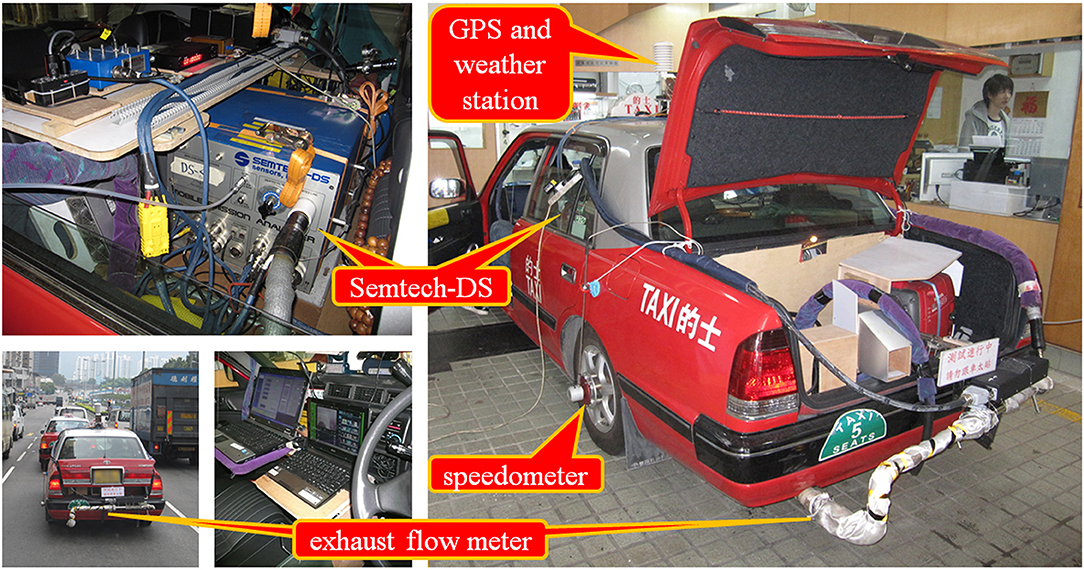
Figure 1. Typical configuration of measurement equipment on a vehicle being measured.

Additionally to on-road measurements, chassis dynamometer warm-start tests have been performed on a Euro 5 LPG taxi, to provide hydrocarbon speciation as well as concentrations of non-regulated pollutants, including ammonia (NH₃) and nitrous oxide (N₂O), using a Fourier-transform infrared spectroscopy (FTIR) gas analyser (Best Instruments BOB-1000FT). An FTIR is a rather heavy, cumbersome, and high power consuming equipment to be carried on road by passenger vehicles, so the chassis dynamometer testing has been the only option. The particular taxi was 5 years old, with mileage of 909,971 km, equipped with its original emission control system. Three different driving cycles were set up on the chassis dyno to represent typical driving conditions in Hong Kong, with their profiles shown in Figure 2. The “urban,” “mix,” and “cruise” cycles had average speeds of 11, 25, and 39 km/h, respectively.

FIGURE 2

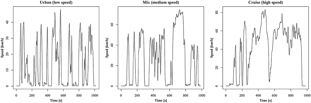
Figure 2. Chassis dynamometer tests driving cycle patterns; urban (left), mix (middle), cruise (right).

Typical automotive LPG fuel used in HK consists of a combination of butane-butylene (70–80%) with the remaining part mostly being propane-propylene, while the total sulfur content in the fuel is limited to 200 ppm (Electrical and Mechanical Services Department of Hong Kong (EMSDHK), 2017).

Results and Discussion

Operation Conditions Characteristics

Figure 3 shows typical recordings of main signals over a trip of mixed operation conditions, graphically shown on the map of Figure 4. The top panel in Figure 3 shows the taxi speed and the altitude profile of the test route, while exhaust (tailpipe) gas temperature and the lambda value (calculated according to ISO16183:2002) are shown in the middle panel, and NO_x, CO, and THC rates are shown in the bottom one. This trip is executed at the city outskirts and involves a mix of driving conditions. The recordings show a typical variability experienced over normal driving conditions, imposed by the traffic and hilly conditions of Hong Kong. The exhaust temperature at the tailpipe varies in the range 120–250°C while the air/fuel ratio range (12.8–20.3 kg air/kg fuel) denotes a rather loose air/fuel ratio control loop. As a result, pollutant emissions seem to significantly vary over the trip, exhibiting a spiky character.

FIGURE 3

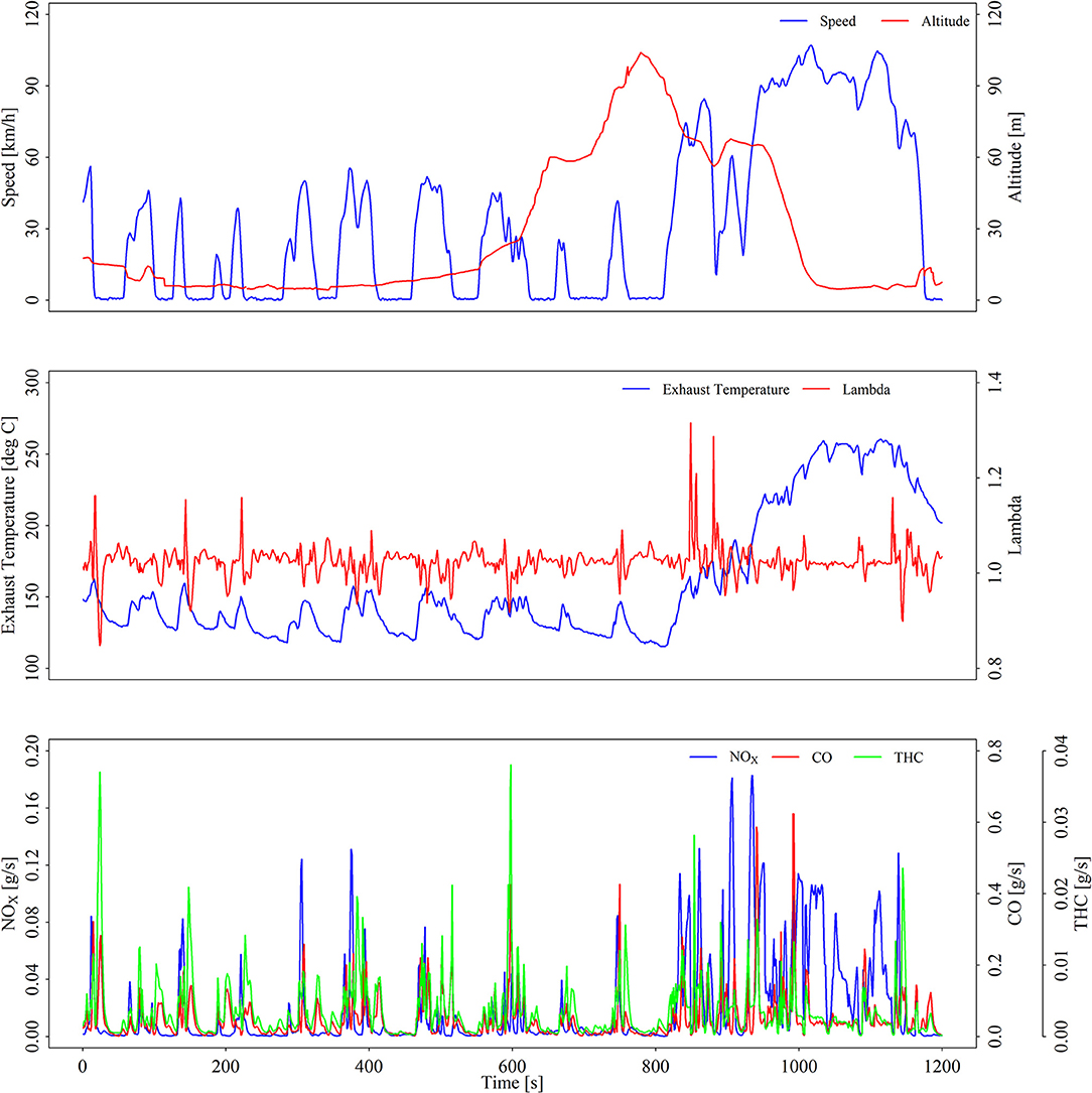
Figure 3. Example of an on-road trip (pre-Euro 4O vehicle) with profiles of recorded signals. Top: speed and altitude, Middle: Exhaust gas temperature and lambda value, Bottom: NO_x, CO, and THC emission mass rates.

FIGURE 4

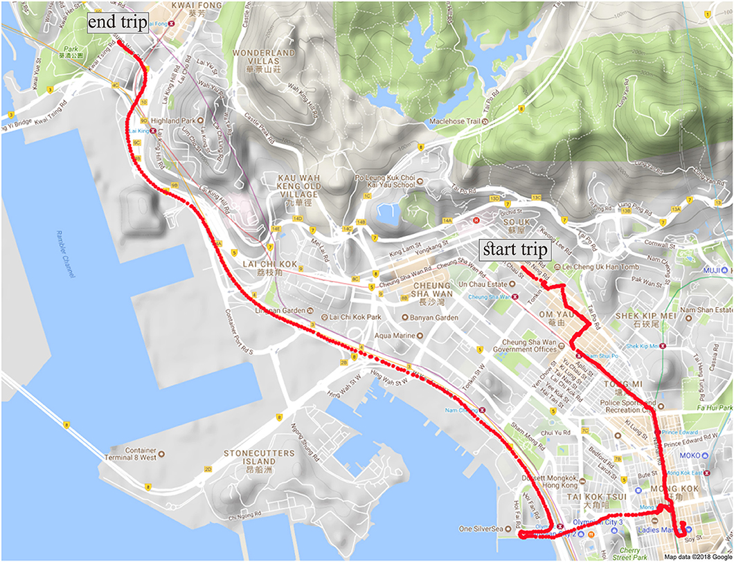
Figure 4. GPS signal spot recordings (red dots) of the trip presented in Figure 3.

Such emission recordings have been conducted for the environmental, terrain and operation conditions summarized in the Supplementary Table 2, in the Supplemental Material. The duration of each trip ranged from 20 to 93 min, with an average duration of 56 min. The total testing duration of the 18 taxis was about 370 h (more than 20 h of testing per vehicle on average), after filtering out incomplete recordings. The altitude of the trips has been estimated by projecting GPS coordinates on the road network, and interpolating over spot height values which are known with approximately 50 m of road distance resolution for all major streets in Hong Kong. In general, driving is conducted at low altitudes but with significant short-distance road slopes and relatively high ambient temperature. Despite the measurement campaign has in total spread over a period of 7 years, mean operation characteristics are rather similar between the different vehicle categories, reflecting the consistency in the conditions these taxis operate on.

The cumulative frequency distribution of the instantaneous speed of all trips is presented in Figure 5. More than 70% of the points are below 50 km/h, while idling operation—corresponding to vehicle speed < 2.5 km/h and an absolute acceleration < 0.1 m/s² (Lau et al., 2011)—is observed for 20% of the time. This is not necessarily representative of the idling frequency of taxis in HK, because the instrumented taxi did not remain behind the target one, if the latter was idling for long. Speeds over 80 km/h correspond to 4% of total points, since the speed limit in the majority of highways in HK is 80 km/h.

FIGURE 5

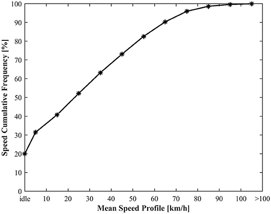
Figure 5. Cumulative frequency distribution of instantaneous speed of the measured taxis.

Mean Emissions and Fuel Consumption Performance

Table 1 presents the mean and standard deviation of NO_x, CO, THC, and FC levels, as well as the ratios over the respective limits, for each technology group. The two statistics are calculated on the basis of the mean emission level of each vehicle within each category. Fuel consumption rates were estimated using the standardized carbon balance equation (UNECE Regulation 101, 2013). All pre-Euro 4 and four out of five Euro 4R vehicles exhibit NO_x emission levels higher than 1 g/km. For comparison, Euro 5 diesel passenger cars, which have been considered of being the highest NO_x light duty vehicle emitters of all times (Ntziachristos et al., 2016), are below this level. Despite absolute levels drop with improving technology, Euro 4 vehicles remain above the corresponding NO_x limit by 12 times on average (min-max: 3–25 times higher). Only Euro 5 LPG taxis are at or even below the corresponding limit, ranging from 59% lower to 82% higher than the limit. Euro 5 LPG taxis are generally younger than Euro 4 ones, i.e., the average test age of the Euro 5 and of the Euro 4 LPG taxis is 3.7 and 7.2 years, respectively.

TABLE 1

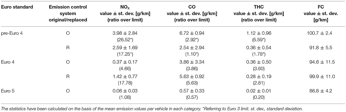
Table 1. Average emission and fuel consumption levels ± standard deviation, and respective ratio over Euro standard limit.

Impact of Emission Control Replacement on Emission Levels

The high standard deviation/mean values in Table 1 suggest large variation of individual vehicle levels or, in other words, a rather heterogeneous vehicle sample in terms of emission level within each technology group. Those vehicles exhibiting NO_x levels more than twice as much as the rest of the vehicles within each group were characterized as “high emitters.” Two of the pre-Euro 4 vehicles were tested both before and after their emission control system (catalyst and lambda sensor) was replaced; one of them characterized as a high-emitter according to the definition given above. In both cases, replacement decreased all pollutant levels, with a higher impact on CO and THC of the normal vehicle (about 90%) than the high emitting one (20–46%). NO_x reductions were mild (15–24%) in both cases. In case of Euro 4 vehicles, one of the tested cars, measured 10 months after its emission control replacement, emitted NO_x at about 40% of the level of the lowest emitting vehicle with original emission control. However, the remaining four Euro 4 vehicles, measured 15 months to 2.5 years after their emission control system replacement, emitted post-replacement about three times higher than the worst emitter with an original emission control system. This limited evidence suggests that the one-off replacement of catalyst and lambda sensor for the taxis does not automatically guarantee that the drop of emissions to normal levels can be sustained for an extended period.

Tests on the pre-Euro 4 and Euro 4 vehicles with replaced emission control were performed 6–19 and 10–31 months, respectively, after replacement had taken place. Only two of the vehicles were tested in less than a year after replacement. A typical taxi conducts on average roughly 150,000 km per year while the emissions control system durability is 80,000 km according to Euro 3 and 100,000 km according to Euro 4 requirements. Post-replacement testing was therefore conducted after replaced catalysts had been significantly aged, beyond their useful life in most cases. This suggests that any environmental benefit of catalyst replacement might already have been exhausted within less than a year after replacement, especially as a poorly maintained engine may contribute to a fast degradation of the TWC and the lambda sensor. The evidence collected here shows the uncertainty in drawing conclusions on the efficacy of emission control replacement. Comparison of pre- and post-replacement levels suggests that emission performance depends on the overall vehicle condition and maintenance history and not only on emission control system condition. This is to be expected from vehicles with average mileage that often exceeded 1 million km. This is similar to evidence collected elsewhere (Díaz et al., 2001) and suggests that retrofitting programmes on captive fleets of spark ignition vehicles should be carefully considered first on pilot samples and, depending on results, consider extending them to a fleet level.

Emission Factors for Meso-Scale Modeling

The Effect of Resolution in Emission Factor Levels

As the emission control replacement status was not a determinant of actual emission level, the remainder of the paper distinguishes vehicles to normal/high emitters and produces separate sets of emission factors, regardless of emission control replacement status. On the other hand, mean traveling speed is considered as a good estimator for emission levels in meso-scale emission modeling, and it is used as an input traffic variable in several emission models (COPERT, MOBILE, EMFAC, etc.) (Franco et al., 2013; Grote et al., 2016). Mean speed has also been used to estimate emissions on a road link-basis for a city network (Lejri et al., 2016). In the past, emission levels over average speed were established by relating mean emission rates with mean speed of driving cycles conducted on the chassis dynamometer (Ntziachristos and Samaras, 2000). Currently, PEMS recordings offer various distance and time-based integration options to develop such a relationship. Time-based integration offers a statistics advantage in using the same sample size to average emission measurements, regardless of mean traveling speed. In distance-based integration, sample size decreases as speed increases, but on the other hand, this may provide an indication for the maximum spatial resolution that the specific EF is applicable to. In our study, different sets of integration intervals were attempted with both methods. Time-based integration was conducted for 60 s and 480 s time intervals while distance-based integration was conducted in steps of 100, 500, and 1,000 m. Figure 6 shows the size of sample recordings in alternative integrating methods, as a function of speed. The sample size in each case is expressed in seconds or in number of recordings, considering one recording per second. The emissions integrated output is better represented with a large sample size, i.e., with high resolution, while low resolution of high integration factor would minimize emissions data fluctuations toward the emission factor development.

FIGURE 6

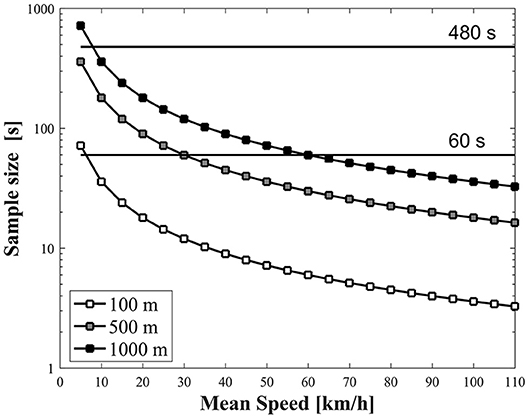
Figure 6. Sample size for different integration methods as a function of mean traveling speed within each sample.

In calculating relevant emission rates, consecutive and non-overlapping time or distance intervals were used. In the past, Smit and Ntziachristos (2012) developed similar intervals based on the moving window principle, which was useful when limited operation profiles were available, such as specific driving cycles in the lab. This method was not considered in the present case, where PEMS data offered adequate and representative variability of actual real-world driving conditions. Using non-overlapping intervals eliminates any potential bias due to the increased autocorrelation, that the moving window approach might introduce.

Figure 7 presents the impact of alternative integration approaches on the speed dependence of Euro 4 NO_x emissions and FC, as an indicative example. Integration over 100 m segments leads to distinctively different NO_x levels in moderate speeds than all other integrations. In this speed range, the 100 m integration corresponds to < 10 s in sample size and this increases the relevant contribution of spiking NO_x events. On the contrary, integration over 480 s delivers very few samples at high speeds, despite more than 20 h of total recording time is conducted per vehicle, and produces an inconsistent emission performance over 60 km/h. Differences between the various methods are less pronounced for FC, however still present. For example, the 100 m resolution leads to 25% higher FC in the sub-10 km/h class than the 500 m resolution.

FIGURE 7

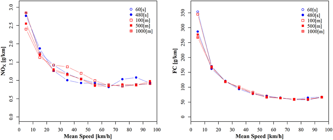
Figure 7. NO_x (left) and FC (right) emissions over mean speed for the alternative integrating options (Euro 4 case study).

A three-way ANOVA test (level of significance, α = 5%) revealed that speed, integration approach and vehicle emission level heterogeneity (within each technology group) are all statistically significant (sig. = 0.000) in explaining emission levels. Subsequent sensitivity analysis showed that speed explained most of the emission levels variation but vehicle emission level heterogeneity can in cases explain more of the total variance, such as in case of Euro 5O vehicles.

The integration approach seems to have an overall lower contribution in emissions variance (Supplementary Table 3). Still, a decisive factor in selecting the integration approach is to minimize the uncertainty in using mean speed to estimate emission levels. Supplementary Table 4, provided in the Supplemental Material, summarizes the mean coefficient of variance (CV) for each integration method and vehicle technology group for NO_x and FC. This has been calculated by binning emissions in 10 km/h speed intervals, calculating the CV in each speed bin and then averaging these CVs across the speed bins. For both time and distance integrations, a clear trend of increasing variance with resolution is observed in Supplementary Table 4. This might be expected, as a finer resolution allows the same mean speed to be reached with many different driving styles. In general, NO_x emissions exhibit a higher variance than FC, irrespective of vehicle group and resolution, as different vehicles within the same group have similar FC levels, and the FC per vehicle across speeds bins is much less sensitive than NO_x.

Selecting an appropriate integration method is therefore a trade-off between uncertainty as resolution increases and availability of test data as resolution decreases, as concluded from Supplementary Table 4 and Figure 6, respectively. The HK traffic network employs road links in the range of 500 m length at maximum. This, together with the fact that the 500 m resolution provides a good compromise in the uncertainty/data availability trade-off, suggest that this may be a suitable resolution for speed-dependant emission factor development on an urban network level.

Vehicle Speed Impact on Emission Levels

The levels of NO_x, CO, THC, and FC over mean speed for each of the vehicle categories considered are presented in Figure 8, for the 500 m distance resolution. These correspond to flat roads, i.e., considering only those road sections where the absolute gradient was < 0.5%. Emissions and FC rather show a monotonic drop with speed, for the speed range considered. The uncertainty in the speed-based functions is assessed using the 95% confidence interval of the mean. Table 2 provides the upper and lower limits of these intervals as the ratio of the half-width of the interval over the respective sample mean. As an example, in the case of pre-Euro 4H vehicles, the real mean NO_x EF (within a speed bin) is expected within the range of ±5% of the respective sample mean, with a confidence of 95%. The interval estimates per vehicle category for FC are narrower when compared to the respective estimates for air pollutants. The NO_x EF estimates are characterized by an average uncertainty within the range of 5–17%, depending on the vehicle group. The CO and THC estimates exhibit a higher level of uncertainty and fall within the range of 7–23 and 5–38%, respectively. The impact of the vehicles emission level heterogeneity on the final estimating uncertainty could be also observed in this case.

FIGURE 8

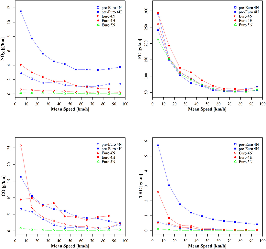
Figure 8. Emissions levels over speed for flat roads for NO_x (upper left), FC (upper right), CO (lower left), and THC (lower right) for the various investigated technologies (distance-integration: 500 m).

TABLE 2

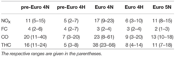
Table 2. Average 95% confidence interval limits of the distance-based emission and FC factors per vehicle category (500 m integrating option) expressed as the percentage (%) ratio of the half-width of the interval over the respective sample mean.

A comparison of Figure 8 emission levels to literature ones is performed, considering that the former are the integrated emission levels over 500 m distance integration, while the latter are not produced from any integration. The comparison of the current study emission levels to the findings of Lau et al. (2011) (using PEMS) shows increased NO_x emission levels at all speed classes, lower CO levels at low speeds and similar levels at higher speeds, and lower THC levels at all speed classes. The comparison of the current study emission levels to the levels presented by Ning and Chan (2007) (using remote sensing), shows higher NO_x and THC emission levels at all speed classes, higher CO levels at low speed classes and lower CO levels at higher speed classes. A more detailed discussion on the comparison with previous studies is performed in section Comparison with previous studies.

Road Slope Impact on Emission Levels

Figure 9 illustrates the slope effect on the levels of NO_x and FC for the pre-Euro 4N vehicles case study. Similar analysis has been performed for all other vehicle categories. The graphs give a comparison of the emission levels over speed for rather steep uphill road slope (>5%) for flat road (absolute slope < 0.5%) and for rather steep downhill road slope (≤5%). The error-bars illustrate the 95% confidence interval of the mean levels. No speed higher than 80 km/h is observed for non-flat roads. Emission levels generally increase with road slope. NO_x emissions in steep uphill are on average 2.9 and 13.3 times higher than in flat and downhill roads, respectively, while the corresponding FC ratios are 1.6 and 2.7, respectively. The error-bars reveal lower uncertainty in flat and downhill driving than in uphill road slope for NO_x, while uncertainty for FC is overall much lower.

FIGURE 9

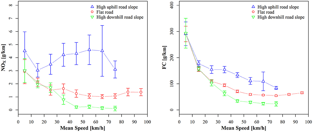
Figure 9. NO_x (left) and FC (right) levels over speed for high uphill road slope (slope > 5%), for flat road (∣slope∣ < 0.5%) and for high downhill road slope (slope < −5%), for the pre-Euro 4N case study (distance-integration: 500 m). Error-bars indicate the 95% confidence interval of the mean levels.

The road slope effect on the levels of NO_x and FC for all vehicle categories are summarized in Figure 10. Uphill and downhill levels are presented as ratios over flat road driving. Uphill driving results to a monotonically increase in emissions with few exceptions, which confirm the high uncertainty of NO_x presented in Figure 9. The opposite is observed for downhill driving. Uphill driving results to significant NO_x increases for pre-Euro 5 vehicles while effects are minimal for Euro 5 ones. This shows that the emission control system of later vehicle technologies is much more effective, over a wider area of driving conditions, than in older vehicles. On the other hand, the impact of road slope on FC is much more consistent among the different vehicle categories.

FIGURE 10

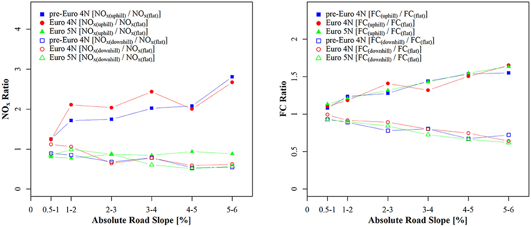
Figure 10. NO_x (left) and FC (right) ratios of uphill (slope >0.5%) and downhill (slope < −0.5%) road slope over flat road (∣slope∣ < 0.5%) as a function of absolute road slope classes for the various investigated technologies (distance-integration: 500 m).

Non-regulated Pollutants

The measurements conducted at the chassis dynamometer provided an indication of the speciation of organic species and non-regulated pollutants, from one Euro 5 taxi. Although this is a single vehicle, emission profiles for late LPG vehicle technologies are missing from the literature despite these are very important for air quality modeling. Figure 11 presents speciation of organics for the three driving cycles. These have been estimated by scaling the FTIR total hydrocarbon concentration to FID THC. Oxygenated and nitrated species concentration have not been scaled, as these are not measured by the FID. The unknown mass illustrated in the Mix cycle, indicates that the total HC mass level calculated from FTIR was lower than the FID THC level, and unspecified species make up the total FID THC level. Otherwise, all three examined cycles exhibit similar HC proportions. C4 (Butane-Butadiene) and CH₄ (Methane) are the predominant species of HC. Interestingly, C3 (Propane-Propylene) content is low, despite that the content of such species in the LPG fuel is 20–30%. C3 species seem therefore to preferentially oxidize over heavier ones during combustion or, later, in the catalyst.

FIGURE 11

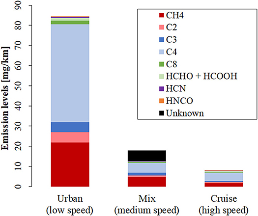
Figure 11. Emission level for the FTIR gas analyser recorded HC species: Methane, C2 (Acetylene, Ethylene, Ethane), C3 (Propylene, Propane), C4 (Butane, Butadiene), C8 (Octane), Formaldehyde and Methanoic Acid, Hydrogen Cyanide, Isocyanic Acid, unknown species.

NH₃ and N₂O are formed in TWC and are directly related to the operating lambda and exhaust temperature. Table 3 presents mean NH₃ and N₂O levels for each driving cycle, which are generally found high compared to the emission levels of previous studies on spark ignition vehicles (Bielaczyc et al., 2013; Suarez-Bertoa et al., 2014, 2015). Both species are expected to form over rich conditions and a degraded catalyst that cannot fully reduce NO_x to nitrogen. Indeed, rich combustion events are observed in the tested vehicle over accelerations and these events coincide with spikes in ammonia and nitrous oxide levels. In TWC systems, N₂O is predominately formed at low temperature levels through incomplete reduction of NO_x by various reductants (Gong and Rutland, 2013; Karavalakis et al., 2016), as also confirmed in the current study at the corresponding low vehicle speeds. The results are indicative but suggest that more attention needs to be given to these species in the exhaust of aged spark ignition vehicles.

TABLE 3

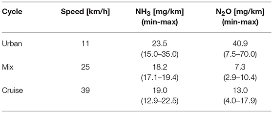
Table 3. Chassis dynamometer tests mean emission levels (min-max indicate the emission level range among test repetitions) of non-regulated pollutants of a Euro 5 LPG taxi.

Comparison With Previous Studies

The comparison of emission levels to previous studies reporting on LPG taxi emissions (Ning and Chan, 2007; Lau et al., 2011) reveals some interesting trends, presented in Table 4. The values express the mean emission levels together with the range of the highest and lowest emitter within each vehicle category. The vehicle allocation in the study of Lau et al. (2011) was rearranged to reflect the latest Euro-standard allocation used by the HK Environmental Protection Department. Therefore, vehicle #2 of that study is actually a Euro 3, and vehicle #3 is a Euro 4 one.

TABLE 4

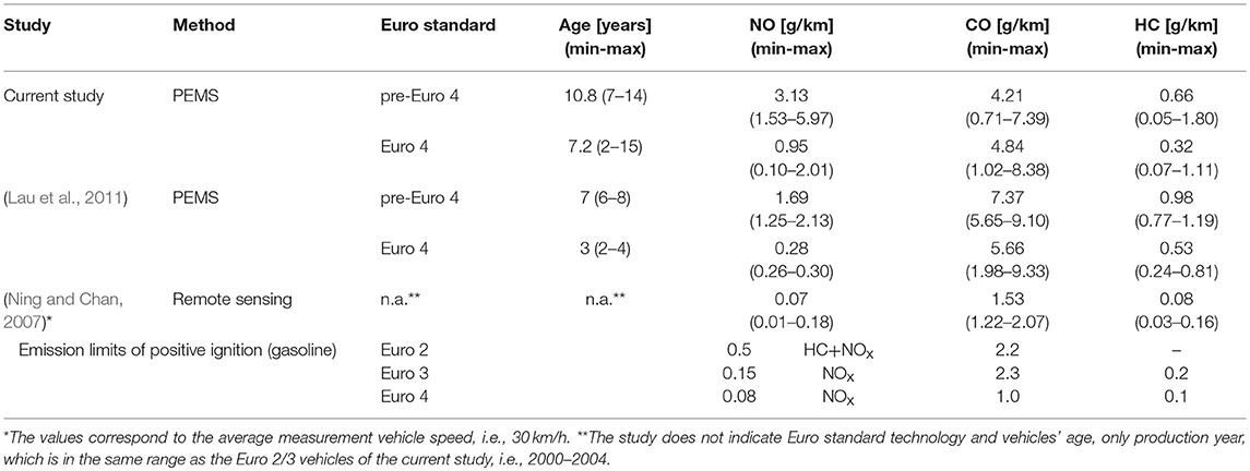
Table 4. Emission levels comparison to previous studies.

The mean NO emission levels of the pre-Euro 4 and Euro 4 vehicles herein are 1.9 and 3.4 times, respectively, higher than what measured by Lau et al. (2011). The emission factors calculated by Ning and Chan (2007), using remote sensing data, are lower than in the current study, with NO exhibiting the largest difference (~45 times lower). The relative difference between our study and the previous ones generally drops with speed for all examined regulated pollutants.

The current results and emission levels reflect comprehensive driving conditions compared to earlier studies, due to the large sample size of the measured taxis and the coverage of a range of driving conditions. Comparison of the levels with the work of Lau et al. (2011) most probably indicates the effect of the mean age increase by 4 years on emission levels between the two studies, using PEMS. For Hong Kong taxis traveling for about 150,000 km per year, this corresponds to more than half a million kilometers. Comparison with the work of Ning and Chan (2007) is more difficult as the remote sensing recordings require instantaneous fuel efficiency assumptions to come up with absolute emission levels and do not take driving dynamics into account (Franco et al., 2013). In this case, part of the substantial emission difference with the current levels may be due to a bias introduced by the fuel efficiency values which were only assumptions in the conversion of the emission data of the remote sensing method, especially as several of the tested vehicles have been shown not to operate on stochiometric combustion.

Summary and Conclusions

This study presented the analysis of the PEMS data collected from 18 LPG taxis from 6 months to 2.5 years after their catalyst and lambda sensor replacement. The examined pollutants include NO_x, CO, and THC, while fuel consumption has been estimated from pollutants emissions. The study attempted to evaluate the impact of catalyst and lambda sensor replacement on pre-Euro 4 (Euro 2 and Euro 3) and Euro 4 emission levels. Due to the high mileage accumulation of taxis, that may exceed the regulatory requirement for catalyst durability within less than a calendar year, the impact of replacement on emissions was overall moderate and variable. Therefore, mean emission levels of LPG taxis from Euro 2 to Euro 4 exceeded emission limits, regardless of catalyst replacement status.

A sample of Euro 5 taxis was also measured with PEMS. In this case, the measured emission levels were mostly lower than the respective regulated limits. However, high NH₃ and N₂O emission levels were reported when measuring a single Euro 5 vehicle in the chassis dynamometer using FTIR with high peaks observed over rich fuel enrichment periods.

In examining integration methods to develop emission factors, the 500 m road segment appeared as a good compromise between sufficient sample size and modeling resolution. Using this resolution, the study demonstrated that both speed and road gradient class have a significant impact on emissions. This dependence is significantly lower for Euro 5 vehicles compared to earlier ones.

The methods followed, and the conclusions of this study are added value to the scientific community, investigating real-world emissions with PEMS of LPG taxis in a metropolitan network and following a meso-scale modeling toward the development of emission factors. Air pollutant emission levels provided are also helpful to policy makers around the world in acknowledging the status of real driving emissions of the specific vehicle category, to synthesize the air pollution puzzle, aiming at the implementation of future air quality targets and RDE legislations.

Author Contributions

The literature study has been performed by GP, CK and supervised by LN. The experimental part has been performed by T-SL, K-LN, H-LW and supervised by CW. The calculation methods followed have been proposed by LN. The statistical analysis has been performed mostly by GP and CK, while LN, T-SL, and CW has also contributed by internally reviewing and advising. The discussion part of the paper has been performed by all co-authors. The manuscript preparation has been performed by GP.

Conflict of Interest Statement

GP and CK were employed by company EMISIA S.A. The contents of this paper are solely the responsibility of the authors and do not necessarily represent official views of the Hong Kong SAR Government.

The remaining authors declare that the research was conducted in the absence of any commercial or financial relationships that could be construed as a potential conflict of interest.

Supplementary Material

The Supplementary Material for this article can be found online at: https://www.frontiersin.org/articles/10.3389/fmech.2018.00019/full#supplementary-material

References

Antes, M., Brindle, R., Kiuru, K., Lloyd, M., Munderville, M., and Pack, L. (2009). Propane Reduces Greenhouse Gas Emissions: A Comparative Analysis. Energetics Incorporated, U.S. Propane Education & Research Council (PERC).

Bielaczyc, P., Szczotka, A., and Woodburn, J. (2013). An overview of cold start emissions from direct injection spark-ignition and compression ignition engines of light duty vehicles at low ambient temperatures. Combust. Engines 154, 48–53. Available online at: http://www.combustion-engines.eu/en/numbers/11/475 (Accessed on 10 May, 2017).

Google Scholar

COWI (2015). State of the Art on Alternative Fuels Transport Systems in the European Union. European Commission DG MOVE - Expert Group on Future Transport Fuels.

Díaz, L., Schifter, I., Rodriguez, R., Avalos, S., López, G., and López-Salinas, E. (2001). Long-term efficiency of catalytic converters operating in Mexico City. J Air Waste Manag. Assoc. 51, 725–732. doi: 10.1080/10473289.2001.10464308

PubMed Abstract | CrossRef Full Text | Google Scholar

Electrical Mechanical Services Department of Hong Kong (EMSDHK) (2017). AutoLPG Specification. Available online at: http://www.emsd.gov.hk/filemanager/en/content_392/AutoLPG_Specification.pdf (Accessed May 10, 2017).

PubMed Abstract

European Alternative Fuels Observatory (EAFO) (2015). LPG Vehicles: Fleet (M1 Category). Available online at: http://www.eafo.eu/vehicle-statistics/lpg (Accessed April 10, 2017).

Franco, V., Kousoulidou, M., Muntean, M., Ntziachristos, L., Hausberger, S., and Dilara, P. (2013). Road vehicle emission factors development: a review. Atmos. Environ. 70, 84–97. doi: 10.1016/j.atmosenv.2013.01.006

CrossRef Full Text | Google Scholar

Gong, J., and Rutland, C. (2013). Three Way Catalyst Modeling With Ammonia and Nitrous Oxide Kinetics for a Lean Burn Spark Ignition Direct Injection (SIDI) Gasoline Engine. Detroit, MI: SAE Technical Paper.

Google Scholar

Grote, M., Williams, I., Preston, J., and Kemp, S. (2016). Including congestion effects in urban road traffic CO₂ emissions modelling: do local government authorities have the right options? Transport. Res. Part D Transport Environ. 43, 95–106. doi: 10.1016/j.trd.2015.12.010

CrossRef Full Text | Google Scholar

Heidt, C., Lambrecht, U., Hardinghaus, M., Knitschky, G., Schmidt, P., Weindorf, W., et al. (2013). On the Road to Sustainable Energy Supply in Road Transport – Potentials of CNG and LPG as Transportation Fuels. DLR-IFEU-LBST-DBFZ report AZ Z14/SeV/288.3/1179/UI40.

Heinze, T., and Zemborski, O. (2016). Abgastests unter realen Fahrbedingungen: Autogas-Pkw im Vergleich mit Benzin- und Diesel-Fahrzeugen - PEMS-Untersuchungen, LPG- und Konventionell betriebenen Pkw, Real-Driving-Emissions-Betrieb und im WLTC-Zyklus. Saarbrücken: HTW automotive powertrain, im Auftrag des Deutschen Verbandes Flüssiggas e. V.

Huss, A., Maas, H., and Hass, H. (2013). Tank-to-Wheels Report Version 4.0 - JEC Well-to-Wheels Analysis: Well-to-Wheels Analysis of Future Automotive Fuels and Powertrains in the European Context. Ispra.

Jeuland, N., and Montagne, X. (2004). EETP: “European Emission Test Programme” Final Report. Institut Francais du Petrole.

Karavalakis, G., Jiang, Y., Yang, J., Hajbabaei, M., Johnson, K., and Durbin, T. (2016). Gaseous and Particulate Emissions from a Waste Hauler Equipped with a Stoichiometric Natural Gas Engine on Different Fuel Compositions. Detroit, MI: SAE Technical Paper.

Google Scholar

Lau, J., Hung, W. T., and Cheung, C. S. (2011). On-board gaseous emissions of LPG taxis and estimation of taxi fleet emissions. Sci. Total Environ. 409, 5292–5300. doi: 10.1016/j.scitotenv.2011.08.054

PubMed Abstract | CrossRef Full Text | Google Scholar

Lejri, D., Can, A., and Leclercq, L. (2016). “Coupling traffic and emission models: dynamic driving speed for emissions assessment”, in 21st International Transport and Air Pollution Conference 2016 (Lyon).

Lim, Y., and Kim, H. (2013). The Evaluation Study on the Contribution Rate of Hazardous Pollutants From Passenger Cars Using Gasoline and LPG Fuel. Bangkok: SAE Technical Paper 2013-01-0068.

Google Scholar

Ning, Z., and Chan, T. L. (2007). On-road remote sensing of liquefied petroleum gas (LPG) vehicle emissions measurement and emission factors estimation. Atmos. Environ. 41, 9099–9110. doi: 10.1016/j.atmosenv.2007.08.006

CrossRef Full Text | Google Scholar

Ntziachristos, L., Papadimitriou, G., Ligterink, N., and Hausberger, S. (2016). Implications of diesel emissions control failures to emission factors and road transport NO_x evolution. Atmos. Environ. 141, 542–551. doi: 10.1016/j.atmosenv.2016.07.036

CrossRef Full Text | Google Scholar

Ntziachristos, L., and Samaras, Z. (2000). Speed-dependent representative emission factors for catalyst passenger cars and influencing parameters. Atmos. Environ. 34, 4611–4619. doi: 10.1016/S1352-2310(00)00180-1

CrossRef Full Text | Google Scholar

Pundkar, A. H., Lawankar, S. M., and Deshmukh, S. (2012). Performance and emissions of LPG fueled internal combustion engine: a review. Int. J. Scie. Eng. Res. 3, 1–7. Available online at: https://www.ijser.org/onlineResearchPaperViewer.aspx?Performance-and-Emissions-of-LPG-Fueled-Internal-Combustion-Engine.pdf (Accessed on 10 May, 2017).

Google Scholar

Smit, R., and Ntziachristos, L. (2012). “COPERT Australia: Developing Improved Average Speed Vehicle Emission Algorithms for the Australian Fleet”, in 19th International Transport and Air Pollution Conference (Thessaloniki).

Google Scholar

Suarez-Bertoa, R., Zardini, A. A., and Astorga, C. (2014). Ammonia exhaust emissions from spark ignition vehicles over the New European Driving Cycle. Atmos. Environ. 97, 43–53. doi: 10.1016/j.atmosenv.2014.07.050

CrossRef Full Text | Google Scholar

Suarez-Bertoa, R., Zardini, A. A., Lilova, V., Meyer, D., Nakatani, S., Hibel, F., et al. (2015). Intercomparison of real-time tailpipe ammonia measurements from vehicles tested over the new world-harmonized light-duty vehicle test cycle (WLTC). Environ. Sci. Pollut. Res. Int. 22, 7450–7460. doi: 10.1007/s11356-015-4267-3

PubMed Abstract | CrossRef Full Text | Google Scholar

UNECE Regulation 101 (2013). E/ECE/324/Rev.2/Add.100/Rev.3. Agreement Concerning the Adoption of Uniform Technical Prescriptions for Wheeled Vehicles, Equipment and Parts Which Can be Fitted and/or be Used on Wheeled Vehicles and the Conditions for Reciprocal Recognition of Approvals Granted on the Basis of these Prescriptions, 48–49.

U. S. Department of Energy (2017). Propane Fuel Basics. Available online at: http://www.afdc.energy.gov/fuels/propane_basics.html (Accessed April 10, 2017).

U. S. Department of Transportation (DOT) Center for Climate Change and Environmental Forecasting (2010). Transportation's Role in Reducing U.S. Greenhouse Gas Emissions, Report to Congress. Washington, DC: Cambridge Systematics.

Vonk, W. A., Verbeek, R. P., and Dekker, H. J. (2010). Emissieprestaties van Jonge Nederlandse Personenwagens Met LPG en CNG Installaties. Delft, TNO Report MON-RPT-2010-01330a.

WLPGA (2016). Autogas Incentive Policies: A Country-by-Country Analysis of Why and How Governments Encourage Autogas and What Works - 2016.