How Thermal Fluctuations Affect Hard-Wall Repulsion and Thereby Hertzian Contact Mechanics

1. Introduction

One of several drawbacks when applying continuum theory to small-scale contact problems, as they occur, for example, in contact mechanics or in colloid science, is that continuum theories often ignore the effect of thermal fluctuations. This can lead to noticeable errors of continuum-theory based predictions for the dependence of displacement or indentation on load when two objects are pressed against each other (Luan and Robbins, 2005, 2006). Temperature can affect mechanical contacts and their interpretation in numerous other ways. For example, the presence of thermal noise generally impedes an unambiguous definition of contact area (Mo et al., 2009; Cheng et al., 2010; Mo and Szlufarska, 2010; Eder et al., 2011; Jacobs and Martini, 2017). In addition, large standard deviations of experimentally measured depinning forces of atomic-force microscope tips have been observed, which were accompanied by unexpectedly large reductions of the depinning force with increasing temperature (Pinon et al., 2016). It is possible that thermal surface fluctuations, which were not included in the modeling of temperature effects on tip depinning, are responsible for a significant reduction of effective surface energy and thereby for a reduction of the depinning force. In fact, it has been shown that thermal fluctuations limit the adhesive strength of compliant solids (Tang et al., 2006). Finally, in the context of colloid science, it may well be that thermal corrections have a non-negligible effect on the surprisingly complex phase diagram of Hertzian spheres (Pàmies et al., 2009). It is therefore certainly desirable to model the effect of thermal fluctuations in a variety of contact and colloid problems.

While thermal fluctuations can be incorporated into simulations with so-called thermostats (Allen and Tildesley, 1987; Frenkel and Smit, 2002), proper sampling can require a significant computational overhead. In addition, some contact solvers do not appear amenable to thermostatting. This concerns in particular those contact-mechanics approaches that optimize the stress field, as done with the classical solver by Polonsky and Keer (Polonsky and Keer, 1999; Müser et al., 2017), rather than the displacement fields in the Green's function molecular dynamics (GFMD) method (Campañá and Müser, 2006; Zhou et al., 2019).

The just-mentioned issues motivated us to investigate how thermal noise affects the mean force F (per unit area) between surfaces as a function of their interfacial separation, or, gap g. The pursued idea is to integrate out the internal degrees of freedom, whereby an areal free-energy density can be defined. The procedure is similar in spirit to the construction of interatomic potentials, for which the (quantum-mechanical ground-state) fluctuations of electrons are integrated out rather than the (thermal) fluctuations of internal elastic degrees of freedom.

In our first attempt on constructing effective surface interactions, we restrict our attention to the oldest, and arguably most commonly used model for the interactions between surfaces, namely a non-overlap constraint. Depending on context and dimension, it can also be called hard-wall, hard-disk, or hard-sphere repulsion, which, by definition is infinitesimally short ranged. Since atoms fluctuate about their equilibrium sites in solids, thermal fluctuations automatically make repulsion effectively adopt a finite range.

The central goal of this study is to quantify the just-described effects and to ascertain if constitutive laws obtained for flat walls can be applied to other systems, in particular to a Hertzian contact. A secondary goal is to identify an analytical expression for the thermal corrections to the load-displacement relation in a Hertzian contact.

2. Model and Numerical Method

2.1. Definition of the Model and Nomenclature

The model consists of a homogeneous, semi-infinite, elastic solid with an originally flat bottom surface, which is pressed down against a continuous, perfectly rigid substrate being fixed in space. The latter, which will also be called indenter, is either perfectly flat, i.e., h(r) = 0, or parabola, in which case $h(\text{r})=-r^2/(2R_{\text{c}})$, where R_c is the radius of curvature. In order to reduce finite-size effects and to simplify both analytical and numerical treatments, periodic boundary conditions are assumed by default within the quadratic, interfacial plane.

The elastic surface is subjected not only to an external load per particle, l, squeezing it down against the indenter but also to thermal fluctuations, as they would occur in thermal equilibrium at a finite temperature T. We restrict our attention to frictionless contacts and small counterface slopes. This allows us to consider only displacements of the elastic surface normal to the interface. As such, the elastic energy of the surface can be written as a functional of the field u(r) according to

$\begin{array}{ll}{U}_{\text{ela}}[u(\text{r})]=\frac{E*A}{4}{\displaystyle \sum _{\text{q}}q}{\left|\tilde{u}(\text{q})\right|}^2.& (1)\end{array}$

Here, u(r) states the z-coordinate of the elastic solid's bottom surface as a function of the in-plane coordinate r = (x, y). E* is the contact modulus, A the (projected) interfacial area, q an in-plane wave vector, and q its magnitude.

$\begin{array}{ll}\tilde{u}(\text{q})=\frac{1}{A}{\displaystyle \int d^2}r{e}^{-i\text{q}·\text{r}}u(\text{r})& (2)\end{array}$

denotes the Fourier transform of u(r). The short-hand notation u₀ = ũ(q = 0) will be used for the center-of-mass coordinate.

For flat indenters, only u₀ will be used to denote the mean distance, or gap, between indenter and the solid surface. Here, we define the displacement d as a function of temperature and load according to

$\begin{array}{ll}d(T,L)\equiv h_{\text{ind}}(r=0)-\langle u(T,L,r\to \infty )\rangle ,& (3)\end{array}$

where 〈u(T, L, r → ∞)〉 is the thermal expectation value that the field u(r) would have (infinitely) far away from the top if the simulation cell were infinitely large. d is sometimes also called interference, as it states an effective penetration of the indenter into the elastic solid.

It is discussed in the literature (Müser, 2014) how to extrapolate accurately u(L, r) to r → ∞ for all those cases, in which an indenter acts relatively localized in the center of a finite simulation cell. However, in the current work, we are interested mostly in the temperature-induced reductions of d, i.e., in the term d_T defined in the expression

$\begin{array}{ll}d=d_0-d_T,& (4)\end{array}$

where d₀ denotes the displacement for an ideal, athermal Hertzian indenter at a given load. In the current work, we compute d_T through the following approximation

$\begin{array}{ll}{d}_T\approx \langle u(T,L,{\text{r}}_X)\rangle -u(0,L,{\text{r}}_X),& (5)\end{array}$

where r_X is the point that is the most distant from the center of the Hertzian indenter. We found that the first three to four digits are accurate in this estimate if the athermal Hertzian contact radius is less than one quarter of the simulation cell's linear dimension. This is because the (true) surface displacement fields converge quite quickly to their asymptotic 1/r form outside the (original) contact radius in the case of short-ranged potentials and because the finite-size corrections to the true surface displacements are not very sensitive to temperature.

The interaction with a counterface is modeled within the Derjaguin approximation (Derjaguin, 1934) so that the surface energy density depends only on the local interfacial separation, or, gap, g(r) = u(r) − h(r), between the surfaces, i.e., the interaction potential is obtained via an integration over the surface energy density γ(g) via

$\begin{array}{ll}{U}_{\text{int}}={\displaystyle {\int }_A{d}^2}r\gamma \{g(\text{r})\},& (6)\end{array}$

In the full microscopic treatment, hard-wall repulsion is assumed, i.e.,

$\begin{array}{ll}\gamma (g)=\{\begin{array}{ll}\infty \hfill & \text{if }g<0\hfill \\ 0\hfill & \text{else }.\hfill \end{array}& (7)\end{array}$

Finally, the probability of a certain configuration to occur is taken to be proportional to the Boltzmann factor, i.e.,

$\begin{array}{ll}\mathrm{Pr}[u(\text{r})]\propto e^{-\beta (U_{\text{ela}}+U_{\text{int}})},& (8)\end{array}$

where β = 1/k_BT is the inverse thermal energy.

One central “observable” in this work is the distance dependence of the mean force per atom, f(u₀), for flat surfaces and finite temperatures. One might want to interpret this function as a cohesive-zone model, or, in the given context better as a repulsive-zone model. Because of the so-called equivalence of ensembles, which is valid for sufficiently large, systems, it does not matter if the separation is fixed and the force measured, or, vice versa.

Note that we will go back and forth between continuous and discrete descriptions of displacement fields. For the discrete description, the elastic solid is partitioned into atoms, which are arranged on a square lattice with the lattice constant Δa. This was done for reasons of simplicity, even if other discretizations are possible, e.g., into a triangular lattice (Campañá and Müser, 2006). Transitions between discrete and continuous representations in real space can be achieved with the substitutions

$\begin{array}{ll}{\displaystyle \sum _n\dots }\leftrightarrow \frac{1}{\Delta a^2}{\displaystyle {\int }_A{d}^2}r\mathrm{...},& (9)\end{array}$

while transitions between summations and integrals in the wavevector domain can be achieved with

$\begin{array}{ll}{\displaystyle \sum _{\text{q}}\dots }\leftrightarrow \frac{A}{{(2\pi )}^2}{\displaystyle \int d^2}q\mathrm{...}.& (10)\end{array}$

To simplify the analytical evaluation of integrals, the square Brillouin zone (BZ) of the surface will be approximated with a circular domain. In this case, the upper cutoff for q is chosen to be $q_{\text{max}}=\sqrt{4\pi }/\Delta a$ as to conserve the number of degrees of freedom with respect to the original BZ.

2.2. Thermal GFMD

GFMD is a method allowing a linearly elastic boundary-value problem to be solved efficiently (Campañá and Müser, 2006; Venugopalan et al., 2017; Zhou et al., 2019). The (discretized) surface displacement field reflects the dynamical degrees of freedom. Elastic interactions are described in terms of appropriate elastic Green's functions, which—in the case of in-plane spatial homogeneity and infinitely large (or periodically repeated) systems—are (block) diagonal in the Fourier representation. The simplest case, which is considered here, is a frictionless contact and a semi-infinite elastic substrate. The equations to be solved in GFMD—using the regular tricks of the trade—are

$\begin{array}{ll}{m}_q\ddot{\tilde{u}}(\text{q})+{\eta }_q\dot{\tilde{u}}(\text{q})+\frac{qE*}{2}\tilde{u}(\text{q})=\tilde{F}(\text{q},t),& (11)\end{array}$

where $\tilde{F}(\text{q},t)$ is the Fourier transform of all external forces acting on the surface atoms. The terms m_q and η_q represent inertia and damping coefficients of different surface modes, which may depend on the wave vector. For isotropic systems, these terms only depend on q but not on the direction of q.

The effect of thermal fluctuations can be cast as random forces, which have to satisfy the fluctuation-dissipation theorem (FDT) (Kubo, 1957). In the given formalism, random forces must have a zero mean, while their second moments must satisfy,

$\begin{array}{ll}\langle \Gamma (\text{q},t)\Gamma (q^{\prime },t^{\prime })\rangle =2{\eta }_{\text{q}}{k}_{B}T{\delta }_{\text{q},q^{\prime }}\delta (t-t^{\prime }),& (12)\end{array}$

assuming discrete atoms, finite domains but continuous times. Here, δ(…) is the Dirac delta function, which can be replaced with ${\delta }_{t,t^{\prime }}/\Delta t$ in a molecular dynamics (MD) simulation, in which the time t is discretized into steps of size Δt.

At this point, GFMD is only used to generate the correct distribution of configurations, which—in a classical system—does not depend on the choice of inertia. As such, the m_q can be chosen at will as far as static observables are targeted. However, in order to reproduce realistic dynamics, appropriate choices for m_q (see also the discussion on quantum effects in section 3.3) and η_q have to be made. In fact, realistic dynamics require the treatment of damping and random noise to have “memory,” as discussed in Kajita et al. (2010). When being interested in fast equilibration, the m_q are better chosen such that the usually slowly equilibrating long-wavelength modes are made light so that characteristic times for different modes coincide as closely as possible (Zhou et al., 2019). In this context, it is also worth mentioning that significant progress has been made recently on GFMD to properly reflect not only true (rather than efficient) dynamics of crystalline solids (Kajita, 2016) but also for truly visco-elastic materials with broad relaxation functions (van Dokkum and Nicola, 2019).

2.3. Hard-Wall Interactions in Thermal GFMD

Non-overlap constraints can be implemented in athermal GFMD by placing any atom, predicted to have penetrated the rigid solid, back onto its surface. This procedure no longer works at finite temperatures. It violates the FDT because the damping that is effectively imposed by this algorithm, is not compensated by a conjugate random force.

The standard way of treating hard-wall or hard-disk interactions is to make it make the time step so large that the next collision between two hard sphere occurs at the end of it. Before proceeding with the time stepping, an ideal, elastic collision is then assumed. This course of action does not appear to be viable for contact mechanics, because it would lead to prohibitively small time steps for large-scale contacts, where several (hundred) thousands of grid points are usually classified as being in contact. Specifically, when doubling the system size N, the typically allowed time step will have to be halved on average so that the asymptotic computational effort would scale with N² rather than with N or N ln N.

2.3.1. Effective Hard-Wall Potentials

An alternative to the standard ways of implementing non-overlap constraints is to allow its violation in a controlled fashion. For example, the true hard-wall interaction can be replaced with a finite-range energy density penalty of the form

$\begin{array}{ll}\gamma (g)=\frac{{\kappa }_{\text{o}}E*\Delta a}{n}{\left(\frac{-g}{\Delta a}\right)}^n\Theta (-g)& (13)\end{array}$

where Θ is the Heavyside step function and κ_o and n are dimensionless parameters. In lose analogy to a Richardson extrapolation, an observable of interest O can be computed for a fixed exponent n but different values of κ_o. Finally, the results can be extrapolated to hard-wall interactions by investigating the asymptotics of O(1/κ) in the limit of 1/κ → 0. Large values of κ_o will limit the time step Δt. However, these limits do not depend on system size. Thus, the numerical effort will scale with O(1/N) rather than with O(1/N²) as is the case when dynamics are based on the more accurate, flexible time-step collision dynamics.

Good numbers for the exponent n and the dimensionless hard-wall stiffness κ_o need to be chosen. In order for the effective hard-wall potential to have a minimal effect on Δt, the (non-negative) exponent n should be as small as possible. However, we would like the force to be a continuous function, for reasons explained at length in any better text book on molecular dynamics (Allen and Tildesley, 1987; Frenkel and Smit, 2002). While these arguments can be somewhat academic when the discontinuities are small, we are going to send κ_o to large numbers resulting in significant force discontinuities. Thus, n must be chosen greater equal two. This appears to make n = 2 the optimal choice.

The next question to be answered is: Given a time step Δt and an exponent of n = 2, what is a good value for κ_o? Here, it is useful to keep in mind that we do not need very accurate dynamics in the “forbidden” overlap zone. The main purpose of the stiff harmonic potential is to eliminate overlap as quickly as possible, i.e., to effectively realize a collision of the particles with the position of the (original) hard wall. However, the stiffness should remain (well) below a critical value above which energy conservation is violated in the absence of a thermostat even when a symplectic integrator, such as the Verlet algorithm, is used. For Verlet, the critical time step for a harmonic oscillator is Δt_c = T/π, where T is the oscillator period, i.e., for Δt < Δt_c, the trajectory may be inaccurate, but the energy is conserved (except for round-off errors). This can be achieved by setting the overlap stiffness to

$\begin{array}{ll}{k}_{\text{o}}={\nu }_{\text{o}}{\pi }^2\frac{m}{d{t}^2}-k_{\text{s}},& (14)\end{array}$

where $k_{\text{s}}=\Delta u^2/(k_{B}T)$, while m is the inertia of the considered degree of freedom. ν_o is a numerical factor, which must be chosen less than unity. At and above the critical value of ν_o = 1, energy conservation would be no longer obeyed in the absence of a thermostat. At the same time, dynamics but also static distribution functions are very inaccurate, even if a thermostat prevents the system from blowing up.

The optimum value for k_o certainly depends on the specific investigated problem. However, the analysis of simple models can provide useful preliminary estimates. This will be done in section 2.3.3.

2.3.2. Approximate Collision Rules

A second possibility to avoid the poor efficiency of exact collision dynamics is to use approximate collision rules and to control the error of the imprecision with the time step. A simple possibility would be to keep Δt fixed in a simulation and to make the deflection of the atom after the regular time stepping. For example, when using velocity Verlet, the following pseudo code could be invoked after a regular time step, in which the constraint was ignored:

if (z violates constraint) then

Z = 2Z_constr-Z

V_Z = -V_Z            (velocity Verlet)

Z_old = 2Z_constr-Z_old  (standard Verlet)

end if

Note that this approach requires extra care to be taken when dynamics are formulated in a wavevector representation, which is usually the case in efficient boundary-element methods. If implemented the following overhead would have to be realized: old positions (or velocities) in real space will then have to be kept in memory. Moreover, two additional Fourier transforms will have to be invoked in each time step, which would double the number of the (asymptotically) most expensive function calls. Since approximate collision dynamics turn out to show similar scaling with Δt in simple models as effective hard-wall repulsion, see section 2.3.3, we did not pursue approximate collision rules further at this point of time in the full contact-mechanics simulations.

2.3.3. Numerical Case Studies

To explore the relative merit of the two proposed hard-wall methods, we investigate the following single-particle problem: an originally free, harmonic oscillator with a (thermal) variance of Δu². This harmonic oscillator is then constrained to have no negative deflections from its mechanical equilibrium site. The analytical solution to this problem stating the force F needed to realize a given constraint is contained in the mean-field approximation to the full elastic problem, which is presented in section 3.2.2. The given constraint of the spring sitting exactly on the hard wall corresponds to a value, where 〈u₀〉 crosses over from its short-range to its long-range asymptotic behavior. Therefore, we see this case as being representative for both scaling regimes.

In essence, the problem we investigate corresponds to the choice where k_BT, k, and m are used to define the unit system, which makes Δu² being unity (in units of k_BT/k) as well. The default time step that we use for the free oscillator is 2π/30, i.e., 30 time steps per period. The damping coefficient is chosen to be γ = 1, whereby the free harmonic oscillator is slightly underdamped. While this choice is not necessarily ideal, it still tends to be effective for a fast equilibration, irrespective of whether the temperature is zero or finite. Results for the convergence of how the estimate for the mean displacement u₀ approaches the exact value with decreasing time step Δt are shown in Figure 1.

FIGURE 1

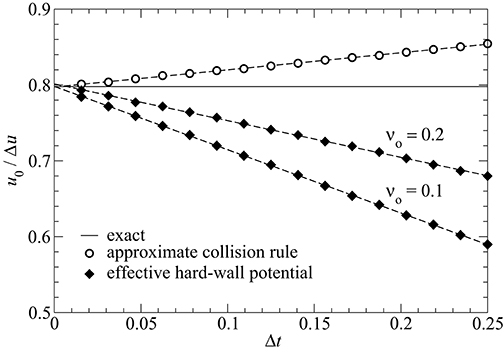
Figure 1. Mean displacement u₀ as a function of time step Δt when using (a) approximate collision rules (open circles) and (b) harmonic effective hard-wall potentials (closed diamonds) for two different values of ν_o, see Equation (14). Dashed lines show linear fits, the solid line the exact, analytical solution. The equilibrium site of the spring is placed at u_s = 0, moreover $\Delta u^2=k_{B}T=1$.

At a given value of Δt, the approximate collision rules clearly outperform the approximate hard-wall interactions. However, u₀ has leading-order corrections of order Δt in both approaches. With the choice ν_o = 0.1, the asymptotic result for the parabolic, effective hard-wall potential has an accuracy of better than 1%, which should be accurate enough for most purposes. In both approaches, simulations must be run at two different values of Δt, say e.g., at Δt = 0.25 and Δt = 0.15 in order to perform a meaningful Δt → 0 extrapolation. In a full contact-mechanics simulation, the number of required Fourier transforms doubles when using the approximate collision rules, which in turn leads to increased stochastic errors given a fixed computing time contingent. For this reason, but also because approximate collision rules require significantly more coding—in particular when averaging wall-surface forces from collisions when using wavevector dependent inertia—we decided to use the harmonic, effective hard-wall potential for the full contact-mechanics simulations.

3. Theory

The main purpose of this section is to identify an analytical expression for the thermal expectation value of an interfacial force per atom f(u₀) as a function of their mean separation u₀ in the case of a hard wall. This will be done by defining the partition function Z(N, β, u₀) of a fluctuating surface in front of a wall, which is linked to the free energy through the relation ${F}(k_{B}T,u_0)=-k_{B}T\text{ ln }Z(\beta ,u_0)$. The mean force between hard wall and elastic surface can then be calculated from

$\begin{array}{ll}f=-\frac{1}{N}\frac{\partial {F}(N,k_{B}T,u_0)}{\partial u_0}.& (15)\end{array}$

Minor errors in the treatment presented below appear in numerical coefficients that result, for example, by having approximated the Brillouin zone of a square with a sphere, or, by having replaced a discrete set of wave vectors (finite system) with a continuous set (infinitely large system). However, these and related approximations are controlled, because errors resulting from them can be estimated and they could even be corrected systematically.

3.1. The Statistical Mechanics of a Free Surface

Since the free surface is the reference state, we start with its discussion. An important quantity, in particular in a mean-field approach, is the variance of atomic displacements due to thermal noise. For a fixed center-of-mass coordinate, it is defined as the following thermal expectation value:

$\begin{array}{ll}\Delta u^2\equiv \langle {\left\{u(\text{r})-\tilde{u}(0)\right\}}^2\rangle .& (16)\end{array}$

It can be evaluated in its wavevector representation in a straightforward manner. Specifically,

$\begin{array}{ll}\Delta u^2={\displaystyle \sum _{q^{\prime }}\langle |\tilde{u}(q^{\prime }){|}^2\rangle }& (17)\end{array}$

$\begin{array}{ll}\approx \frac{A}{{(2\pi )}^2}{\displaystyle \int d^2}q\frac{2k_{B}T}{qE*A}& (18)\end{array}$

$\begin{array}{ll}\approx \frac{2}{\sqrt{\pi }}\frac{k_{B}T}{E*\Delta a},& (19)\end{array}$

where we made use of equipartition for harmonic modes, see also Equation (29).

Of course, up to the prefactor of $2/\sqrt{\pi }\approx 1.1284$, which is very close to unity, Equation (19) follows directly from dimensional analysis. However, in a quantitative theory, we wish to know and perhaps to understand its precise value. A numerical summation over a square BZ assuming a square real-space domain with N atoms reveals that Δu² can be described by

$\begin{array}{ll}\Delta u^2=\left(1.1222-\frac{1.24}{\sqrt{N}}\right)\frac{k_{B}T}{E*\Delta a},& (20)\end{array}$

with more than three digits accuracy if $\sqrt{N}>512$. This result is fairly close to the analytical result based on a BZ, which is approximated as sphere.

Assuming discretization down to the atomic scale of Δa ≈ 2.5 Å yields a root-mean square (rms) height of

$\begin{array}{ll}\Delta u\approx 1.5\sqrt{\text{GPa}/E*}\text{ Å}& (21)\end{array}$

at room temperature. Thus, for soft-matter systems, the effect of thermal fluctuations is not necessarily non-negligible at room temperature. The dominant restoring forces to height fluctuation at short scales will then be due to surface tension rather than due to elasticity (Xu et al., 2014). However, it might be possible to suppress those effects when immersing the surfaces into an appropriate liquid, e.g., crosslinked polyethylene glycol (PEG) into uncrosslinked PEG.

An outcome of Equation (19) is that the fluctuations are dominated by the small scales. In the simplest approximation, which can be made in direct association with the Einstein model of solids, each surface atom is coupled harmonically to its lattice site with a spring of stiffness $k_{\text{E}}=k_{B}T/\left\{(N-1)\Delta u^2\right\}$. In reality, i.e., in less than infinite dimensions, there is always a correlation of thermal height fluctuations.

To deduce an estimate for the distance over which height fluctuations are correlated, we calculate the thermal displacement autocorrelation function (ACF) C_uu(r). It can be defined and evaluated to obey:

$\begin{array}{ll}{C}_{uu}(\Delta r)=\langle u(\text{r})u(\text{r}+\Delta \text{r})\rangle & (22)\end{array}$

$\begin{array}{ll}\approx \frac{1}{2{\pi }^2}\frac{k_{B}T}{qE*}{\displaystyle {\int }_0^{\sqrt{4\pi }/\Delta a}d}q{\displaystyle {\int }_0^{2\pi }d}\phi e^{iqr\cos \phi }& (23)\end{array}$

$\begin{array}{ll}=\frac{1}{\pi }\frac{k_{B}T}{rqE*}{\displaystyle {\int }_0^{\sqrt{4\pi }r/\Delta a}d}(qr)J_0(qr)& (24)\end{array}$

$\begin{array}{ll}=\frac{2k_{B}T}{qE*}\frac{\sqrt{4\pi }r}{\Delta a}{{}_{1}F}_2\left(\frac{1}{2};1,\frac{3}{2};\frac{-\pi r^2}{\Delta a^2}\right)& (25)\end{array}$

$\begin{array}{ll}\approx \{\begin{array}{ll}\frac{2k_{B}T}{\sqrt{\pi }E*\Delta a}+{O}(r^2)\hfill & \text{ for }r\to 0\hfill \\ k_{B}T/(\pi qE*r)\hfill & \text{ for }r\to \infty ,\hfill \end{array}& (26)\end{array}$

where J₀(x) is the Bessel function of the first kind and ₁F₂(…) is a generalized hypergeometric function. Unfortunately, the result obtained analytically this way shows Helmholtz ringing at intermediate values of r (i.e., within a substantial range of Δu), which is why the exact analytical solution for C_uu(r) is of little practical use, except in the two limiting cases r = 0 and r → ∞. Helmholtz ringing is generally a consequence of sharp cutoffs in the wave vector domain. Interestingly, it persists even for a square BZ when the exact expectation values for |ũ(q)|² are used and the correlation function C_uu(r) is extended to the continuous domain between the lattice positions. The validity of these claims is demonstrated in Figure 2.

FIGURE 2

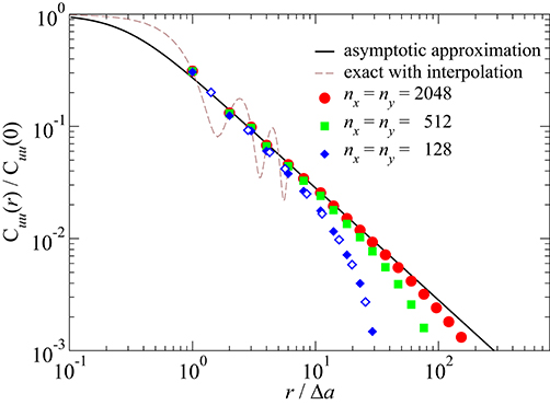
Figure 2. The radial displacement ACF C_uu(r)—normalized to its value at r = 0—as a function of distance r: asymptotic approximation given in Equation (27) (black line), exact correlation function along the [10] direction with interpolation between non-lattice sites (dashed brown line), numerically exact results for systems of size 2,048 × 2,048 (red circles), 512 × 512 (green squares), and 128 × 128 (blue diamonds). They were also obtained for the [10] direction, except for the open symbols, which refer to the [11] direction.

A quite reasonable approximation or rather generalization of C_uu(r) to a continuous function can be made by constructing the simplest expression with the correct asymptotic behaviors summarized in Equation (26):

$\begin{array}{ll}{C}_{uu}(r)\approx \frac{2}{\sqrt{\pi }}\frac{k_{B}T}{E*}\frac{1}{{(\Delta a^2+4\pi r^2)}^{1/2}}.& (27)\end{array}$

As can be seen in Figure 2, this asymptotic approximation is quite reasonable already at a nearest-neighbor spacing of r = Δa and has errors of less than 5% (in the limit of large N) for larger values of r. While numerical results for finite systems in Figure 2 include predominantly data for r parallel to [1, 0], similar results are obtained for other directions as well, as demonstrated examplarily for the [1, 1] direction of the N = 128 × 128 lattice.

The asymptotic ACF has decayed to approximately 30% of its maximum value at the nearest-neighbor distance. This means that the displacements of adjacent lattice sites are essentially uncorrelated.

The last property of interest used in the subsequent treatment is the partition function of a free surface (fs):

$\begin{array}{ll}{Z}_{\text{fs}}(\beta )={\displaystyle \prod _{\text{q}}\frac{{\lambda }_q}{\sqrt{2\pi \Delta u^2(q)}}}& (28)\end{array}$

with

$\begin{array}{ll}\Delta u^2(q)=\frac{2k_{B}T}{qE*A}.& (29)\end{array}$

${\lambda }_q=h/\sqrt{2m_q{k}_{B}T}$ represents the thermal de Broglie wavelength of a surface mode. It reflects the ideal-gas contribution of the momenta conjugate to the ũ(q) to the partition function. As long as E* is small compared to the ambient pressure and as long as temperature is kept constant, the sole purpose of including λ_q into the calculation is to render the partition function dimensionless. This is why a precise determination of m_q is not needed at this point, even if it might be an interesting topic in itself and of relevance for a quantum-mechanical treatment, which is discussed in section 3.3.

In the mean-field (Einstein solid) approximation, the partition function simplifies to

$\begin{array}{ll}{Z}_{\text{mf}}(\beta )={\left(\frac{{\lambda }_{\text{mf}}}{\sqrt{2\pi \Delta u^2}}\right)}^N,& (30)\end{array}$

with Δu having been introduced in Equation (19) and λ_mf being a mean-field de Broglie wavelength.

3.2. Interaction of a Thermal, Elastic Surface With a Flat Wall

In this section, we investigate the statistical mechanics of an elastic surface in front of a flat, hard wall. To this end we derive expressions for the partition function of the system, from which the mean force between surface and wall (at fixed mean separation) can be derived in a straightforward fashion. Different mean-field strategies will be pursued toward this end. They turn out to be quite accurate in different asymptotic limits of the full problem.

3.2.1. First Mean-Field Approximation

The arguably simplest analytical approach to the contact problem is an adaptation of the so-called Einstein solid, which was already alluded to in section 3.1, to surface atoms. We first do it such that a degree of freedom is a hybrid of an atom in real space and a delocalized, ideal sine wave. Specifically, we first assume that elastic energy of an individual atom reads

$\begin{array}{ll}{v}_{\text{ela}}^{\text{mf}}(u)=\frac{k_{B}T}{2\Delta u^2}{u}^2.& (31)\end{array}$

In order to maintain a zero expectation value of u, it is furthermore assumed that the interaction energy with a counterface placed at a distance u₀ from the atom's mean position is given by

$\begin{array}{ll}{v}_{\text{sub}}^{\text{mf}}(u)=\frac{\Delta a^2}{2\pi }{\displaystyle {\int }_0^{2\pi }d}\phi \gamma (u_0+u\cos \phi ).& (32)\end{array}$

This means, an oscillation of an atom entails an undulation. With this assumption, u₀ automatically corresponds to the atom's mean position.

The excess free energy per particle $\Delta {F}/N$ for a fixed center-of-mass position satisfies

$\begin{array}{ll}{e}^{-\beta {F}/N}=\frac{1}{\sqrt{2\pi \Delta u^2}}{\displaystyle {\int }_{-\infty }^{\infty }\text{}}\text{}du{e}^{-\beta \{v_{\text{ela}}^{\text{mf}}(u)+v_{\text{sub}}^{\text{mf}}(u)\}},& (33)\end{array}$

where the term “excess” refers to the change of the free energy relative to that of a free surface. For hard-wall interactions, the integral in Equation (33) can be evaluated to be

$\begin{array}{ll}\begin{array}{l}{e}^{-\beta {F}/N}=\frac{1}{\sqrt{2\pi \Delta u^2}}{\displaystyle {\int }_{-u_0}^{u_0}\text{}}\text{}du{e}^{-\beta v_{\text{ela}}(u)}\hfill \\ =\text{erf}\left(\frac{u_0}{\sqrt{2}\Delta u}\right).\hfill \end{array}& (34)\end{array}$

Hence,

$\begin{array}{ll}\frac{{F}}{N{k}_{B}T}=-\text{ln }\left\{\text{erf}\left(\frac{u_0}{\sqrt{2}\Delta u}\right)\right\}& (35)\end{array}$

$\begin{array}{ll}\approx \{\begin{array}{ll}-\text{ ln }\left(\sqrt{\frac{2}{\pi }}\frac{u_0}{\Delta u}\right)\hfill & \text{for }{u}_0<\Delta u/2\hfill \\ \frac{\Delta u}{\sqrt{\pi }{u}_0}{e}^{-u_0^2/(2\Delta u^2)}\hfill & \text{for }{u}_0>2\Delta u.\hfill \end{array}& (36)\end{array}$

For reasons of completeness, the force predicted from this first mean-field approximation is stated as:

$\begin{array}{ll}{f}_{\text{mf1}}(u_0)=\sqrt{\frac{2}{\pi }}\frac{k_{B}T}{\Delta u}\frac{\text{exp}\{-u_0^2/(2\Delta u^2)\}}{\text{erf}\{{\text{u}}_0\text{/}(\sqrt{\text{2}}\Delta \text{u})\}}.& (37)\end{array}$

In the limit of u₀ → 0, repulsion diverges proportionally with 1/u₀, while it decays slightly quicker than exponentially in $u_0^2$ for separations u₀ ≫ Δu. Both limiting behaviors are confirmed in the results section, albeit, with a prefactor of a little less than one half for large separations.

3.2.2. Second Mean-Field Approximation

Another mean-field approach would be to abandon the evaluation of the interaction in terms of an undulation and to introduce a Lagrange parameter, i.e, an external force f divided by the thermal energy, ensuring u to adopt the desired value of u₀. Thus, the probability of a displacement u to occur satisfies

$\begin{array}{ll}\mathrm{Pr}(u)\propto e^{-{(u-u_0)}^2/(2\Delta u^2)-\beta f(u-u_0)}\Theta (u),& (38)\end{array}$

where f needs to be chosen such that 〈u〉 = u₀ so that the lattice position of the particle u_eq is situated at $u_{\text{eq}}=u_0+\beta f\Delta u^2$. At u_eq, there is no elastic restoring force in the spring. The requirement 〈u〉 = u₀ automatically leads to the following self-consistent equation for f:

$\begin{array}{ll}\beta f\Delta u=\sqrt{\frac{2}{\pi }}\frac{\text{exp }\left\{-\frac{{(\beta f\Delta u^2-u_0)}^2}{2\Delta u^2}\right\}}{1-\text{erf}\left(\frac{\beta f\Delta u^2-u_0}{\sqrt{2}\Delta u}\right)}.& (39)\end{array}$

This line of attack leads to similar results for the f(u₀) at small u₀ as the first mean-field approach. However, for large u₀ the predicted force turns out half that of the first mean-field approximation. In fact, the second mean-field theory turns out to be a quite reasonable approximation to the numerical data for any value of Δu, see the results and discussion presented in section 4.

3.2.3. Probabilistic Approach

The exact expression for the excess free energy of an elastic body in front of a hard wall can be defined by a path integral,

$\begin{array}{ll}{e}^{-\beta {F}(u_0^{\prime })}=\frac{1}{Z_A}{\displaystyle \int {D}}[u(\text{r})]\delta \left(u_0^{\prime }-u_0\right)e^{-\beta v_{\text{tot}}[u(\text{r})]},& (40)\end{array}$

where ${D}\left[u(\text{r})\right]$ denotes an integral over all possible displacement realizations and

$\begin{array}{ll}{Z}_A={\displaystyle \int {D}}[u(\text{r})]\delta \left(u_0-u_0^{\prime }\right)e^{-\beta v_{\text{ela}}[u(\text{r})]}.& (41)\end{array}$

In the case of hard-wall repulsion, the r.h.s. of Equation (40) is easy to interpret: It represents the relative number of configurations that are produced with the thermal equilibrium distribution of a free surface (fs), whose maximum displacement is less than u₀, i.e.,

$\begin{array}{ll}{e}^{-\beta {F}(u_0)}={\langle \mathrm{Pr}(u_{\text{max}}<u_0)\rangle }_{\text{fs}},& (42)\end{array}$

This insight defers the problem of having to solve the path integral in Equation (40) to an exercise in probability theory: determine the likelihood of $N^{\prime }=N\Delta a^2/\Delta A_{\text{c}}$ independent Gaussian random number with mean zero and variance Δu² to be less than u₀. Here ΔA_c is the correlation area for the displacements. Given that C_uu(Δr) has decayed to a few 10% at nearest-neighbor distances, it can only be marginally larger than Δa².

For large values of N′, the distribution of maximum values u_max = max{u(r)} converges to the Gumbel distribution, also known as the generalized extreme value (gev) distribution type-I (David and Nagaraja, 2003). It is given by

$\begin{array}{ll}\mathrm{Pr}(u_{\text{max}})=\frac{1}{{\beta }_{\text{gev}}}{e}^{-\left(e^{-z}\right)}& (43)\end{array}$

with

$\begin{array}{ll}z=\frac{u_{\text{max}}-{\mu }_{\text{gev}}}{{\beta }_{\text{gev}}},& (44)\end{array}$

where μ_gev is the mode of the Gumbel distribution, i.e., the most likely value for u_max to occur, and β_gev a parameter determining the shape of the distribution. For a normal Gaussian distribution Φ_G(u/Δu), they are given by

$\begin{array}{ll}\frac{{\mu }_{\text{gev}}}{\Delta u}=\sqrt{2}{\text{ erf}}^{-1}\left(1-\frac{2}{N^{\prime }}\right)& (45)\end{array}$

$\begin{array}{ll}\frac{{\beta }_{\text{gev}}}{\Delta u}=\frac{1}{N^{\prime }\cdot {\Phi }_{\text{G}}({\mu }_{\text{gev}}/\Delta u)}& (46)\end{array}$

in the limit of large N′. Here erf⁻¹(…) stands for the inverse function of the error function (David and Nagaraja, 2003).

In fact, Figure 3 shows that the distribution of u_max as produced with GFMD and by taking the maximum value of N′ = 0.92N independent random numbers are essentially identical and that both can be approximated quite well with the Gumbel distribution. If setting N′ = N, the (open) symbols in Figure 3 would shift by roughly half their symbol size to the right. As expected, discrepancies between the Gumbel distribution and the numerical data decrease with increasing N′.

FIGURE 3

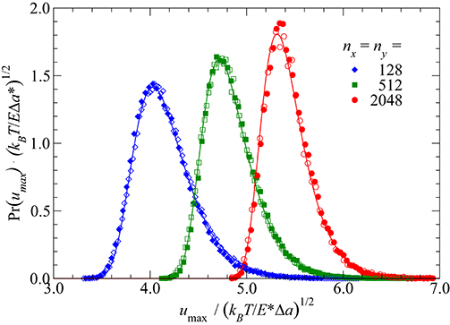
Figure 3. Distribution of maximum displacements for different system sizes as obtained from GFMD (closed symbols). Considered system sizes are N = 128 × 128 (diamonds), 512 × 512 (squares), 2048 × 2048 (circles). Comparison is made to the distribution of the maximum of N′ = 0.92N independent random numbers of mean zero and variance Δu (open symbols) as well as to the corresponding Gumbel distribution.

Rather than relying on the Gumbel distribution, one might as well write down the exact probability of one positive Gaussian random variable (grv) to be less than u₀ and take the result into the N′/2-th power. (On average, there are N′/2 positive grv's, whose value may not exceed u₀. The negative grv's are irrelevant with respect to the violation of the violation of the non-overlap constraint.) In this approximation,

$\begin{array}{ll}\mathrm{Pr}(u_{\text{max}}<u_0)={\left\{\text{erf}\left(\frac{u_0}{\sqrt{2}\sigma }\right)\right\}}^{N^{\prime }/2}.& (47)\end{array}$

and therefore

$\begin{array}{ll}\Delta {F}=-\frac{N^{\prime }{k}_{B}T}{2}\text{ln }\left\{\text{erf}\left(\frac{u_0}{\sqrt{2}\Delta u}\right)\right\}.& (48)\end{array}$

This result turns out to apply to large separations, that is, to u₀/Δu ≫ 1. The functional form of ${F}(u)$ is identical to the one obtained in the first mean-field variant, except for the prefactor, which is reduced by a little more than a factor of two.

3.3. Handling Quantum Effects

Throughout this paper, it is assumed that thermal vibrations are classical. In reality, atoms are quantum mechanical, which enhances their fluctuations about their equilibrium sites. Differences between classical and quantum systems can matter when the Debye temperature is clearly larger than the ambient temperature. In this section, we briefly sketch how the quantum-mechanical fluctuations could be modeled rigorously but also suggest an alternative approach. The latter is easily implemented and should be reasonably accurate except for very large squeezing forces.

A rigorous treatment could be based on path-integral techniques (Berne and Thirumalai, 1986; Müser, 2002), in which quantum-mechanical (QM) point particles are represented in terms of classical ring polymers. The course of action would be an acquisition of the proper Green's function with similar fluctuation formulae as in the original GFMD paper (Campañá and Müser, 2006), while simulating (half) solids and acquiring elastic tensor or stiffness elements as done, for example, in Schöffel and Müser (2001). For a harmonic system, the stiffness of the various modes would be identical in the classical and the quantum system so that the most important variable to be determined would be the q-dependent inertia m_q of the surface modes. It would have to be selected such that it yields the correct zero-point vibration in a path-integral augmented GFMD simulation. The latter would benefit from replacing the free-particle propagator in so-called imaginary time with one that is symmetry-adopted for hard walls as done in Müser and Berne (1997).

In classical systems, Δu is dominated by the shortest wavelength modes. This will be even more so for quantum systems, because modes show greater quantum effects at short than at long wavelengths. In other words, the model of an Einstein solid should provide a reasonable approximation for the true, quantum-mechanical variance $\Delta u_{\text{QM}}^2$ of a free elastomer. In this approximation, the effective stiffness of a spring coupling the z-coordinate of a surface atom to its lattice site is E*Δa, divided by a factor very close to 1.12, which we consider negligible in the present discussion. If m is the mass of a surface atom, the associated eigenfrequency would be ${\omega }_0=\sqrt{E^{*}\Delta a/m}$. Thus, the temperature-dependent internal energy of an Einstein mode is obtained as U = ℏω₀ coth{ℏω₀/(2k_BT)}/2, where ℏ is the reduced Planck constant, see any textbook on statistical mechanics. Since U = 2〈V_pot〉 for the quantum or classical harmonic oscillator, it can be deduced that

$\begin{array}{ll}\Delta u_{\text{QM}}^2\approx \frac{\Delta u^2}{2k_{B}T\tanh \{\hslash {\omega }_0/(2k_{B}T)\}}.& (49)\end{array}$

If quantum effects need to be included, the value of $\Delta u_{\text{QM}}^2$ would have to replace that of Δu² in any application of the method. The treatment would not be exact, because the wavefunction and thus the quantum-mechanical probability density go to zero at the hard-wall constraint. This would lead to enhanced repulsion, in particular at large compression, for which we expect repulsion to diverge more quickly than with 1/u₀ because of the uncertainty prinple. Yet, using $\Delta u_{\text{QM}}^2$ instead of the classical Δu² would be roughly analogous to a first-order perturbation theory and thereby represent quantum effects accurately for separations u₀ ≳ Δu_QM.

3.4. Thermal Hertzian Contacts

3.4.1. Preliminary Considerations

At small temperatures, the relative leading-order corrections to the zero-temperature displacement u₀(T = 0) can be expected to depend on powers of the variables defining the problem, i.e.,

$\begin{array}{ll}\frac{d_T}{d_0}\propto {\left(\frac{R_{\text{c}}}{\Delta a}\right)}^{\alpha }{\left(\frac{E*R_{\text{c}}^2}{L}\right)}^{\beta }{\left(\frac{k_{B}T}{E*R_{\text{c}}^3}\right)}^{\gamma },& (50)\end{array}$

where the contact modulus E* and the contact radius R_c were effectively used to define the units of pressure and length, respectively. With the help of a further dimensional analysis, which can be conducted in a similar fashion as that in Müser (2014), the sum rule

$\begin{array}{ll}\alpha +3\beta -5\gamma =0& (51)\end{array}$

follows immediately for the exponents introduced on the r.h.s. of Equation (50). This relation is valid for a quadratic tip shape, linear elasticity, assuming the interfacial stress is a function of u(r)/Δu with $\Delta u\propto \sqrt{T}$.

The r.h.s. of Equation (50) and the sum rule for exponents in Equation (51) can also be valid at high-temperatures. However, different exponents will apply. At intermediate temperatures, an expansion over terms such as those discussed so far are the only possibility to conform to the dimensional analysis.

3.4.2. Low-Temperature Approximation

At very small temperatures, the stress profile can be expected to differ only marginally from that of the athermal contact. In a perturbative approach to the problem, one could therefore assume that the most important correction to the original Hertzian gap g_H(r) is a constant shift by d_T. The latter can be determined by minimizing the thermal excess energy per atom

$\begin{array}{ll}{e}_T=-d_{T}L+\frac{1}{\Delta a^2}{\displaystyle \int \text{}}\text{}{d}^{2}r{{F}}_{\text{pa}}\left\{g_{\text{H}}(r)+d_T\right\}& (52)\end{array}$

$\begin{array}{ll}\approx -d_{T}L+\frac{2\pi }{\Delta a^2}{\displaystyle {\int }_0^{{\text{a}}_{\text{c}}}\text{}}\text{}drr{{F}}_{\text{pa}}(d_T),& (53)\end{array}$

where ${{F}}_{\text{pa}}\equiv {F}/N$ denotes the hard-wall, free-energy normalized to the atom. The approximation in Equation (53) is motivated by the expectation that the dominant contribution to e_T resides within the original contact area. Minimization of e_T w.r.t. d_T leads to

$\begin{array}{ll}L=\frac{\pi a_{\text{c}}^2}{\Delta a^2}f(d_T)& (54)\end{array}$

$\begin{array}{ll}\approx \frac{\pi a_{\text{c}}^2}{\Delta a^2}\sqrt{\frac{2}{\pi }}\frac{k_{B}T}{\Delta u}\frac{\text{exp }\left(-u_0^2/2\Delta u^2\right)}{\text{erf}({\text{u}}_0\text{/}\sqrt{\text{2}}\Delta \text{u})}& (55)\end{array}$

where the last approximation is only valid at small temperatures. Taylor expanding this last expression leads to

$\begin{array}{ll}\frac{d_T}{d_0}\approx \frac{T}{T*}& (56)\end{array}$

with

$\begin{array}{ll}T*=\frac{L\Delta a^2}{\pi k_B{R}_{\text{c}}}.& (57)\end{array}$

3.4.3. High-Temperature Approximation

At very large temperatures, d_T is in excess of d₀ so that deformations of the elastic solids are very small. In a first-order perturbative approach, it then makes sense to assume the displacement field to be a constant, i.e., to be d_T. In that approximation, individual forces can be simply summed up with a mean gap of $d_{\text{T}}+r_n^2/(2R_{\text{c}})$. Recasting the sum as an integral yields

$\begin{array}{ll}L\approx \frac{N^{\prime }}{2N}\frac{1}{\Delta a^2}{\displaystyle \int \text{}}\text{}{d}^{2}r{f}_{\text{mf1}}\left(d_T+\frac{r^2}{2R_{\text{c}}}\right)& (58)\end{array}$

$\begin{array}{ll}\approx L_0\frac{\Delta u}{d_T}{e}^{-d_T^2/(2\Delta u^2)}& (59)\end{array}$

with

$\begin{array}{ll}{L}_0=\sqrt{\frac{2}{\pi }}\frac{N^{\prime }}{N}\frac{k_{B}T{R}_{\text{c}}}{\Delta a^2}.& (60)\end{array}$

Equation (59) can be solved for d_T with the help of the Lambert W function W(x) ≈ ln x − ln ln x for x ≫ 1:

$\begin{array}{ll}\frac{d_T}{\Delta u}\approx \sqrt{W\left(\frac{L_0^2}{L^2}\right)}.& (61)\end{array}$

4. Results

4.1. Potential of Mean Force for a Flat Hard Wall

In this section, we investigate to what extent the three approaches introduced in section 3.1 reproduce accurate, numerical results for the thermal repulsive-zone model. To this end, we chose units such that E* = 1 and Δa = 1 and consider different values of u₀/Δu, which is the only dimensionless variable for the given problem besides the system size, which is varied as well.

Figure 4 compares GFMD data to the various approximative approaches introduced in section 3. The first mean-field approach appears to be asymptotically exact for small u₀, while the approach based on the law of large numbers seems to be asymptotically exact for large u₀. In between these two regimes, there is a smooth transition between them. This transition is reflected quite well by the second mean-field approach. Unfortunately, we did not identify a closed-form analytical expression for it, which would nevertheless be nice to have when implementing a potential of mean force into a simulation. However, as is demonstrated in Figure 4, simple switching functions introduced next allow one to approximate numerical data reasonably well.

FIGURE 4

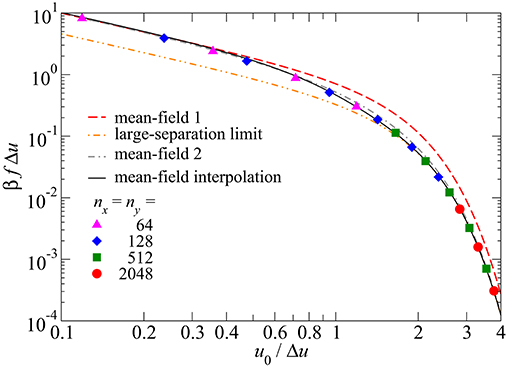
Figure 4. Mean force f, in units of 1/βΔu, as a function of normalized mean separation u₀/Δu, where Δu represents the height standard deviation of a surface atom in the absence of a counterface.

Since both force-distance asymptotic dependencies have the same functional form and since the transition between them is quite continuous, it is relatively easy to come up with switching functions allowing the numerically determined free energy to be approximated reasonably well. Defining ${{F}}_{\text{mf}1}$ through the free-energy expression in Equation (35), this is done via

$\begin{array}{ll}{F}(u_0)\approx w_1(u_0){{F}}_{\text{mf1}}(u_0)+w_2(u_0)\Delta {F}& (62)\end{array}$

with the weighting functions

$\begin{array}{ll}{w}_1(u_0)=\frac{1}{2}\left\{\frac{N^{\prime }}{N}+\left(2-\frac{N^{\prime }}{N}\right)e^{-u_0^2/\Delta u^2}\right\}& (63)\end{array}$

$\begin{array}{ll}{w}_2(u_0)=e^{-u_0^2/\Delta u^2}\left\{1-\tanh (u_0/\Delta u)\right\}& (64)\end{array}$

The numerical value for $\Delta {F}$ turned out to be $\Delta {F}=-N^{\prime }{k}_{B}T/2$. The forces f(u) in a coarse-grained description are obtained as negative derivative by differentiating the r.h.s. of Equation (62). The resulting expression corresponds to the numerical GFMD data for systems with n_x = n_y ≥ 128 with maximum errors less than 10%, at least when taking the exact value for Δu².

In terms of an efficient implementation of the method, we recommend to use tabulated expressions for f(u) for intermediate values of u and the asymptotic expressions for u ≪ Δu and u ≫ Δu.

4.2. Hertzian Indenter

We now consider a Hertzian indenter as transferability test for our effective potential. In addition, the effects that thermal fluctuations have on the load displacement relation are explored along with an analysis of how to meaningfully define a contact area in the presence of thermal fluctuations.

The solution of the continuous displacement field has no dimensionless number if the contact radius a_c is taken to be the unit of length. However, a_c/Δa starts to matter as soon as it is no longer large compared to unity. Since discreteness effects are a different topic discussed elsewhere (Müser, 2019), a_c/Δa is chosen sufficiently large so that the discrete problem reflects the continuous Hertz contact reasonably well.

To test the applicability of the thermal repulsive-zone model in the realm of Hertzian contact mechanics, the following parameters were chosen as useful defaults after some trial and error: R_c = 256 Δa and a normal load of L = 131 E*Δa² leading to a_c ≈ 30 Δa within regular Hertzian contact mechanics. In the athermal Hertzian contact, the mean contact pressure turns for these parameters is p ≈ 0.049 E*. Results for the stress profile at a temperature of $k_{B}T=0.2E^{*}\Delta a^3$ are shown in Figure 5.

FIGURE 5

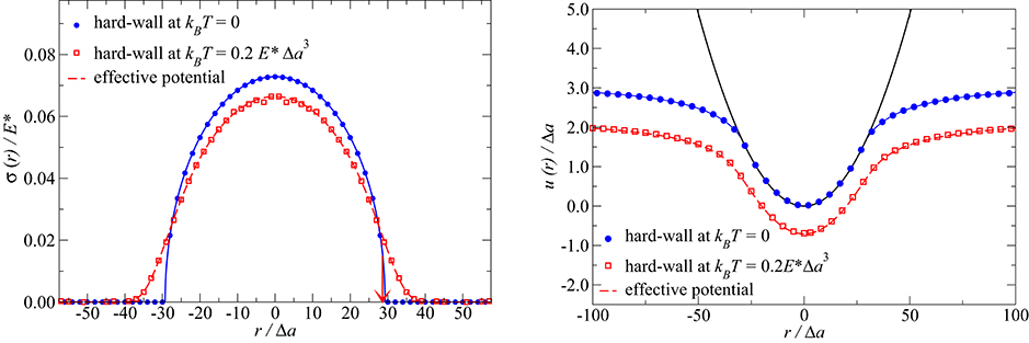
Figure 5. (Left) Interfacial stress σ as a function of distance r from the symmetry axis in a Hertzian contact geometry. The (blue) circles reflect zero temperature data from the hard-wall overlap potential. The full (blue) line represents the analytical solution to the Hertz problem. The (red) open squares show finite-temperature data from full simulations, while the (red) dotted line shows zero-temperature simulations, in which, however, the effective potential was constructed to reflect thermal vibrations at the given temperature. The arrow marks the point of largest slope for the thermal indenter. (Right) Displacement field u(r) as a function of distance r from the symmetry axis.

An interesting but perhaps also obvious outcome of the data presented in Figure 5 is that there is no abrupt transition from finite to zero contact stress, once thermal fluctuations are finite. This observations is of relevance when discussing the concept of “true contact area.” Since collisions in a hard-wall potential are instantaneous, the probability of observing two (finite) surfaces to be in contact has a statistical measure of zero, so that the instantaneous contact area could be argued to be (almost) always zero. Contact exists only in the isolated moments of time at which collisions take place. However, during these isolated moments of time, the forces between surfaces is infinitely large such that time averaging yields a distribution which resembles the well-known Hertzian stress profile; the smaller the temperature the closer the stress profiles between original and finite-temperature stress profiles.

The question of how to meaningfully define (repulsive) contact area when repulsion has a finite range and adhesion is neglected arises naturally. In a recent paper (Müser, 2019), it was proposed to define the contact line (or edge) to be located, where the gradient of the normal stress has a maximum slope. In the current example, this leads to a reduction of the contact radius of order 1%, which is significantly less than the reduction of approximately 30% of the normal displacement in the given case study.

In contrast to contact radii, force and displacement can be defined unambiguously. Thermal noise will reduce the interference d by d_T due to the effectively finite range of the repulsion, as discussed in the definition of the model in section 2.1. Since the description for an athermal Hertzian contact is scale free —in the sense that the functional form for stress and displacement are independent of any parameter defining a Hertzian contact– the function f(T) ≡ d_T/d₀ must have a universal shape if Δa ≪ a_c. This is because the thermal repulsive zone model for hard-wall repulsion is a scale-free function of the gap divided by Δu. Figure 6 reveals that results on the thermal displacement for different Hertzian contact realizations can indeed be collapsed quite closely onto a single master curve $\Xi (T/\tilde{T})$ defined through

$\begin{array}{ll}{d}_T={\tilde{d}}_0\Xi (T/\tilde{T}),& (65)\end{array}$

where

$\begin{array}{ll}{\tilde{d}}_0={\left(\frac{R_{\text{c}}L}{E*\Delta a^3}\right)}^{-\frac{1}{3}}{d}_0& (66)\end{array}$

and

$\begin{array}{ll}\tilde{T}={\left(\frac{L}{E*R_{\text{c}}^2}\right)}^{\frac{2}{3}}\frac{E*\Delta a^3}{k_B}.& (67)\end{array}$

The master curve shown in Figure 6 reveals asymptotic regimes at low and at high temperatures, respectively. They can be approximated with power laws. However corrections logarithmic in temperature need to be made at low temperature to obtain quantitative agreement over broad temperature ranges. We find numerically that

$\begin{array}{ll}\Xi (t)\approx \{\begin{array}{ll}t(1-\ln t)\hfill & \text{ for }t\ll 1\hfill \\ 1.727\sqrt{t}\{1+\ln (t)/6\}\hfill & \text{ for }0.1<t<{10}^4\hfill \end{array}.& (68)\end{array}$

Inserting the low-temperature approximation of the master curve into Equation (65) and reshuffling terms yields

$\begin{array}{ll}\frac{d_T}{d_0}\approx \frac{T}{T*}\left(1-\ln \frac{T}{\tilde{T}}\right)& (69)\end{array}$

for $T\ll \tilde{T}$. This means that the low-temperature treatment presented in section 3.4.2 obtained the correct linear term, but failed to predict the logarithmic corrections, which become very large at small ratios $T/\tilde{T}$. Before discussing the origin of those corrections, we wish to emphasize that there are indeed two characteristic temperatures for the Hertzian contact, namely T* and $\tilde{T}$.

FIGURE 6

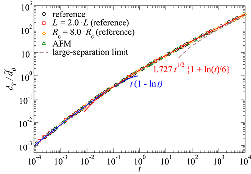
Figure 6. Reduced thermal displacement $d_{\text{T}}/{\tilde{d}}_0$ as a function of reduced temperature $t=T/\tilde{T}$ for different Hertzian contact realizations. The default model (black circles) is defined in the method section. In one case, load was increased by a factor of two (red squares), and in another case, the radius of curvature was increased by a factor of eight (orange diamonds) with respect to the default values. Finally, values found for blunt atomic-force microscope (AFM) tips were also considered: Δa = 2.5 Å, R_c = 200 nm, E* = 100 GPa, and L = 200 nN (green triangles). Solid blue and red line show the low- and intermediate-temperature approximation from Equation (68). The dashed brown line represents the high-temperature limit of Equation (61).

The suspicion that significantly better results at small $T/\tilde{T}$ are obtained when extending the integration domain in Equation (53) back to radii beyond the athermal contact radius turns out incorrect. The main reason for the deviations lies in the assumption of a constant thermal shift of the thermal displacement. Figure 7 reveals that the thermal shift far away from the indenter is noticeably larger than at r = 0 and that discrepancies grow (logarithmically) with decreasing temperature. Since the simple treatment allows one to rationalize why d_T is (roughly) linear in temperature, we decided to keep the discussion of the low-temperature limit.

FIGURE 7

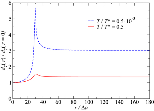
Figure 7. Spatially resolved thermal displacement d_T(r) normalized to the its value at r = 0 at two different reduced temperatures T/T* for the default model. Lower and upper temperature are indicated by dashed blue and solid red lines, respectively.

Before investigating the magnitude of thermal displacements in real units and not just in reduced units, we briefly comment on the intermediate-temperature behavior. Most importantly, we wish to emphasize that the approximation made in Equation (68) for t > 0.1 is only valid on the shown domain and that it does not extend to t → ∞.

However, from a practical point of view, it appears virtually impossible to design a real-laboratory experiment, in which the asymptotic high-temperature regime of t > 10³ could ever be reached. The only possible exception coming to our minds would involve the use of hagfish slime. It has extraordinarily small elastic moduli of order 0.02 Pa (Ewoldt et al., 2011), though the values of Δa to be used in a continuum model would be clearly in excess of the atomic scale, because hagfish slime stops being homogeneous well above the atomic scale. Since the contact mechanics of hagfish slime and related systems is somewhat of a niche application, we would argue that the analytical solution given in Equation (61) is merely a nice mathematical result and that the t > 0.1 approximation made in Equation (68) can be considered the high-temperature limit for all other purposes.

One may wonder how the master curve shown in Figure 6 translates into a d(T) dependence when real units rather than reduced units are used. To answer that question, the expansions obtained previously are represented again for a moderately hard-matter (E* = 1 GPa) and a soft-matter (E* = 50 MPa) system, see Figure 8 and further validated by additional GFMD simulations. In both cases, a radius of curvature of R_c = 50 nm was assumed and the load was chosen such that the ratio of maximum Hertz pressure to E* was in the order of 0.1%, i.e., a load where plastic deformation can be assumed to be minor.

FIGURE 8

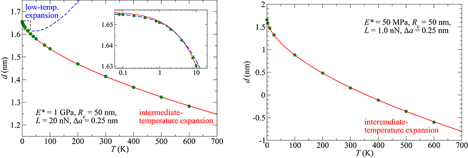
Figure 8. Displacement as a function of temperature at fixed load for a moderately hard-matter (left, E* = 1 GPa) and a soft-matter (right, E* = 50 MPa) system. Symbols indicate the results from GFMD simulations, while blue and red lines represent the low-temperature and intermediate-temperature approximations, respectively.

Figure 8 reveals that both studied systems qualify as being clearly in the intermediate-temperature regime at room temperature. Relative corrections of the normal displacement for the stiffer system are rather minor but non-negligible for the soft-matter system. This observation brings us to the next and final question, which is addressed in Figure 9, namely to what extent do thermal correction affect the load-displacement relation? After all, most indentation experiments are done at constant temperature and varying load rather than at constant load and varying temperature. Combining Equations (65–67) with the intermediate-temperature expansion of Equation (68) and the analytical solution for the displacement-load relation in a Hertzian contact, leads to the following relation:

$\begin{array}{ll}{d}_T=d_T^{\text{ref}}\left\{1-\frac{1}{9}\text{ln }\left(L/L^{\text{ref}}\right)\right\}& (70)\end{array}$

with $d_{\text{T}}^{\text{ref}}\approx 1.426\Delta u$ and

$\begin{array}{ll}{L}^{\text{ref}}={\left(\frac{k_{B}T}{E\Delta a^3}\right)}^{3/2}E*R_{\text{c}}^2.& (71)\end{array}$

In other words, the elastomer surface is effectively shifted by a little less than 1.5 times the thermal standard deviation of its smallest-scale surface fluctuations. The effects of load are minuscule as they enter only logarithmically in the ninth' root of the load.

FIGURE 9

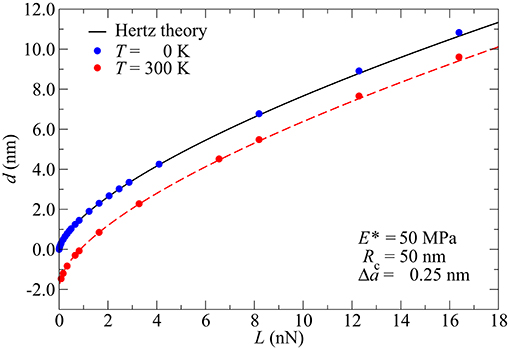
Figure 9. Displacement as a function of load at zero and room temperature for a moderately hard-matter for a soft-matter (E* = 50 MPa) system. Symbols indicate the results from GFMD simulations, while blue and red lines represent the low-temperature and intermediate-temperature approximations, respectively.

Figure 9 confirms that the thermal fluctuation in most real Hertzian contacts should lead to corrections that appear as almost constant shifts to the eye, even for soft-matter systems, for which the absolute shifts can be relatively large. In the case study presented in Figure 9, the thermal shift reads d_T ≈ 1.2 at a load of L ≈ 16 nN and barely more at a much reduced load d_T ≈ 1.7 at a load as small as L ≈ 0.16 nN In order for the d_T correction to acquire twice the value compared to that at 16 nN, the compressive force in our example would have to be as small as L ≈ 20 fN, which is scarcely measurable. For the reasons of completeness, we state that the range of validity of the intermediate-temperature approximation of 0.1 < t < 10⁴ demonstrated in Figure 6 translates to a range of loads of 0.15 < L/nN < 1.5 · 10⁴ for the specific examples studied here. Upper and lower limits are well beyond loads that could be meaningfully applied or measured experimentally for the system of question while measuring the normal displacement with high resolution.

5. Summary

In this work, we analyzed the effect that thermal fluctuations can have on contact mechanics in the case of hard-wall interactions. To this end, we first demonstrated that thermal surface fluctuations are dominated by short wavelengths undulations. They smear out the originally infinitesimally short-range repulsion to a finite range of $\Delta u\approx \sqrt{k_{B}T/(E^{*}\Delta a)}$. The functional form of the repulsive force was derived analytically and shown to diverge inversely proportionally with the interfacial separation u₀ at small u₀ but to decay slightly more quickly than exponentially in $-u_0^2/(2\Delta u^2)$ at separations clearly exceeding Δu.

To come to these results, the Green's function molecular dynamics (GFMD) technique was generalized to include thermal noise. Particular emphasis was placed on the question how to handle (the original) hard-wall interactions in the simulations. We found that replacing the hard-wall overlap constraint with a stiff harmonic potential produces satisfactory results if simulations are done at different values for the stiffness and extrapolation is made to infinite stiffness. The GFMD results are described very well with different mean-field approximations to the problem, which made it possible to identify a highly-accurate, closed-form analytical expression for the distance-force relation a flat, thermal elastomer interacting with a flat, rigid substrate.

It may be important to note that each microscopic interaction law requires the coarse-graining to be done for that particular interaction. For example, if thermal fluctuations were to be treated in a Dugdale model (Dugdale, 1960) (e.g., hard-wall constraint plus a constant adhesive stress acting up to a finite range), results for the hard-wall constraint cannot be simply incorporated, but a new parametrization of thermal effects has to be done.

Application of our methodology to Hertzian contacts revealed that thermal fluctuations can induce non-negligible shifts in the normal displacement. As a zero-order approximation, it can be assumed that the thermally induced shift of a Hertzian indenter is a little less than 1.5 times the thermal standard deviation of surface positions of a free, unconstrained surface. Corrections turn out to depend only logarithmically on the ninth' root of the normal load. Thus, thermal noise leads to a shift of the load-displacement curve that is roughly equal to the root-mean-square fluctuation of surface atoms but almost independent of the load. As a referee of this manuscript noticed: This picture is simple and easily understandable intuitively aposteriori, but by no means trivial and understandable in advance. The result of an essentially load-independent displacement shift may, in part, explain why Hertzian contact models often apply all the way down to the nanoscale: Essentially constant shifts remain unnoticed.

We expect similar results for randomly rough and other hard-wall indenters as for Hertzian contacts, because the thermal shift for the Hertz contact is relatively insensitive to the radius of curvature. However, the effect of thermal fluctuations will be more important in the case of short-range adhesion. Given the results from this study, quite noticeable adhesion reductions may be expected when its range is in the order of or less than the thermal displacement Δu. Future studies are ongoing elucidating the reduction of adhesion due to thermal vibrations.

Data Availability Statement

The datasets generated for this study are available on request to the corresponding author.

Author Contributions

MM, YZ, and AW developed the code and analyzed the results. YZ run the simulations. MM performed the analytical calculations. MM and YZ wrote the paper.

Funding

Salaries of AW and YZ were paid in parts by the DFG through grant MU 1694/5-2 and in parts by Saarland University while the research was conducted. A University grant will cover the APF.

Conflict of Interest

The authors declare that the research was conducted in the absence of any commercial or financial relationships that could be construed as a potential conflict of interest.

References

Allen, M., and Tildesley, D. (1987). Computer Simulation of Liquids. Oxford: Clarendon.

Google Scholar

Berne, B. J., and Thirumalai, D. (1986). On the simulation of quantum systems: path integral methods. Annu. Rev. Phys. Chem. 37, 401–424. doi: 10.1146/annurev.pc.37.100186.002153

CrossRef Full Text | Google Scholar

Campañá, C., and Müser, M. H. (2006). Practical Green's function approach to the simulation of elastic semi-infinite solids. Phys. Rev. B 74:075420. doi: 10.1103/PhysRevB.74.075420

CrossRef Full Text | Google Scholar

Cheng, S., Luan, B., and Robbins, M. O. (2010). Contact and friction of nanoasperities: effects of adsorbed monolayers. Phys. Rev. E 81:016102. doi: 10.1103/PhysRevE.81.016102

PubMed Abstract | CrossRef Full Text | Google Scholar

David, H. A., and Nagaraja, H. N. (2003). Order Statistics. 2003. New York, NY: Wiley.

Google Scholar

Derjaguin, B. (1934). Untersuchungen über die Reibung und Adhäsion, IV. Kolloid-Zeitschrift 69, 155–164. doi: 10.1007/BF01433225

CrossRef Full Text | Google Scholar

Dugdale, D. (1960). Yielding of steel sheets containing slits. J. Mech. Phys. Solids 8, 100–104. doi: 10.1016/0022-5096(60)90013-2

CrossRef Full Text | Google Scholar

Eder, S., Vernes, A., Vorlaufer, G., and Betz, G. (2011). Molecular dynamics simulations of mixed lubrication with smooth particle post-processing. J. Phys. 23:175004. doi: 10.1088/0953-8984/23/17/175004

PubMed Abstract | CrossRef Full Text | Google Scholar

Ewoldt, R. H., Winegard, T. M., and Fudge, D. S. (2011). Non-linear viscoelasticity of hagfish slime. Int. J. Non-Lin. Mech. 46, 627–636. doi: 10.1016/j.ijnonlinmec.2010.10.003

CrossRef Full Text | Google Scholar

Frenkel, D., and Smit, B. (2002). Understanding Molecular Simulation: From Algorithms to Applications, volume 1 of Computational Science Series, 2nd Edn. San Diego, CA: Academic Press.

Google Scholar

Jacobs, T. D. B., and Martini, A. (2017). Measuring and understanding contact area at the nanoscale: a review. Appl. Mech. Rev. 69:060802. doi: 10.1115/1.4038130

CrossRef Full Text | Google Scholar

Kajita, S. (2016). Green's function nonequilibrium molecular dynamics method for solid surfaces and interfaces. Phys. Rev. E 94:033301. doi: 10.1103/PhysRevE.94.033301

PubMed Abstract | CrossRef Full Text | Google Scholar

Kajita, S., Washizu, H., and Ohmori, T. (2010). Approach of semi-infinite dynamic lattice Green's function and energy dissipation due to phonons in solid friction between commensurate surfaces. Phys. Rev. B 82:115424. doi: 10.1103/PhysRevB.82.115424

CrossRef Full Text | Google Scholar

Kubo, R. (1957). Statistical-mechanical theory of irreversible processes. I. General theory and simple applications to magnetic and conduction problems. J. Phys. Soc. Jpn. 12, 570–586. doi: 10.1143/JPSJ.12.570

CrossRef Full Text | Google Scholar

Luan, B., and Robbins, M. O. (2005). The breakdown of continuum models for mechanical contacts. Nature 435, 929–932. doi: 10.1038/nature03700

PubMed Abstract | CrossRef Full Text | Google Scholar

Luan, B., and Robbins, M. O. (2006). Contact of single asperities with varying adhesion: comparing continuum mechanics to atomistic simulations. Phys. Rev. E 74:026111. doi: 10.1103/PhysRevE.74.026111

PubMed Abstract | CrossRef Full Text | Google Scholar

Mo, Y., and Szlufarska, I. (2010). Roughness picture of friction in dry nanoscale contacts. Phys. Rev. B 81:035405. doi: 10.1103/PhysRevB.81.035405

CrossRef Full Text | Google Scholar

Mo, Y., Turner, K. T., and Szlufarska, I. (2009). Friction laws at the nanoscale. Nature 457, 1116–1119. doi: 10.1038/nature07748

PubMed Abstract | CrossRef Full Text | Google Scholar

Müser, M. (2002). On new efficient algorithms for PIMC and PIMD. Comput. Phys. Commun. 147, 83–86. doi: 10.1016/S0010-4655(02)00221-7

CrossRef Full Text | Google Scholar

Müser, M. H. (2014). Single-asperity contact mechanics with positive and negative work of adhesion: influence of finite-range interactions and a continuum description for the squeeze-out of wetting fluids. Beilstein J. Nanotechnol. 5, 419–437. doi: 10.3762/bjnano.5.50

PubMed Abstract | CrossRef Full Text | Google Scholar

Müser, M. H. (2019). Elasticity does not necessarily break down in nanoscale contacts. Tribol. Lett. 67:57. doi: 10.1007/s11249-019-1170-y

CrossRef Full Text | Google Scholar

Müser, M. H., and Berne, B. J. (1997). Circumventing the pathological behavior of path-integral monte carlo for systems with coulomb potentials. J. Chem. Phys. 107, 571–575. doi: 10.1063/1.474442

CrossRef Full Text | Google Scholar

Müser, M. H., Dapp, W. B., Bugnicourt, R., Sainsot, P., Lesaffre, N., Lubrecht, T. A., et al. (2017). Meeting the contact-mechanics challenge. Tribol. Lett. 65:118.

Google Scholar

Pàmies, J. C., Cacciuto, A., and Frenkel, D. (2009). Phase diagram of Hertzian spheres. J. Chem. Phys. 131:044514. doi: 10.1063/1.3186742

CrossRef Full Text | Google Scholar

Pinon, A. V., Wierez-Kien, M., Craciun, A. D., Beyer, N., Gallani, J. L., and Rastei, M. V. (2016). Thermal effects on van der waals adhesive forces. Phys. Rev. B 93:035424. doi: 10.1103/PhysRevB.93.035424

CrossRef Full Text | Google Scholar

Polonsky, I., and Keer, L. (1999). A numerical method for solving rough contact problems based on the multi-level multi-summation and conjugate gradient techniques. Wear 231, 206–219. doi: 10.1016/S0043-1648(99)00113-1

CrossRef Full Text | Google Scholar

Schöffel, P., and Müser, M. H. (2001). Elastic constants of quantum solids by path integral simulations. Phys. Rev. B 63:224108. doi: 10.1103/PhysRevB.63.224108

CrossRef Full Text | Google Scholar

Tang, T., Jagota, A., Chaudhury, M. K., and Hui, C.-Y. (2006). Thermal fluctuations limit the adhesive strength of compliant solids. J. Adhes. 82, 671–696. doi: 10.1080/00218460600775781

CrossRef Full Text | Google Scholar

van Dokkum, J. S., and Nicola, L. (2019). Green's function molecular dynamics including viscoelasticity. Model. Simulat. Mater. Sci. Eng. 27:075006. doi: 10.1088/1361-651X/ab3031

CrossRef Full Text | Google Scholar

Venugopalan, S. P., Müser, M. H., and Nicola, L. (2017). Green's function molecular dynamics meets discrete dislocation plasticity. Model. Simulat. Mater. Sci. Eng. 25:065018. doi: 10.1088/1361-651X/aa7e0e

CrossRef Full Text | Google Scholar

Xu, X., Jagota, A., and Hui, C.-Y. (2014). Effects of surface tension on the adhesive contact of a rigid sphere to a compliant substrate. Soft Matt. 10, 4625–4632. doi: 10.1039/C4SM00216D

PubMed Abstract | CrossRef Full Text | Google Scholar

Zhou, Y., Moseler, M., and Müser, M. H. (2019). Solution of boundary-element problems using the fast-inertial-relaxation-engine method. Phys. Rev. B 99:144103. doi: 10.1103/PhysRevB.99.144103

CrossRef Full Text | Google Scholar