Iterative Tomography: A Key to Providing Time-Dependent 3-D Reconstructions of the Inner Heliosphere and the Unification of Space Weather Forecasting Techniques

Introduction

The bulk of the particles within the solar wind, a hot, strongly turbulent plasma produced by the Sun, are accelerated up to speeds of about 400 km s⁻¹ or more. On average, it takes about 4 days for individual features in the solar wind to travel 1 AU from the Sun to reach the Earth. Transient structures such as Coronal Mass Ejections (CMEs) are usually thousands of times larger than Earth at 1 AU and often travel several times faster than 400 km s⁻¹. A few reach Earth in less than one day. These transient heliospheric phenomena can strongly perturb the geomagnetic field in the near-Earth environment by means of magnetic reconnection and storm triggering when they arrive at 1 AU. They can also accelerate solar energetic particles (SEPs) as well as affect their transport in the heliosphere. In particular, CMEs can modify the surrounding medium by introducing changes in the direction and strength of the interplanetary magnetic field (IMF). The so-called ambient solar wind is not without structure; its features emanate primarily from specific locations on the Sun. Solar locations where magnetic fields open outward have solar winds that are accelerated about twice as fast as the ecliptic average. At times of solar minimum, winds that emanate from the solar poles that are open are also twice as fast and can extend down across the ecliptic. As the Sun rotates, these different features move out primarily radially to provide a spiral structure with faster plasma that merges with generally denser and slower moving portions causing Stream Interaction Regions (SIRs).

Remotely sensed interplanetary scintillation (IPS) data (Hewish et al., 1964) to study the inner heliosphere was pioneered in Cambridge, England (e.g., Houminer 1971; Hewish and Bravo, 1986; Behannon et al., 1991). IPS data from radio observatories near the University of California, San Diego (UCSD), and those from the Solar-Terrestrial Environment Laboratory (STELab), now the Institute for Space-Earth Environmental Research (ISEE), at Nagoya University, Japan, enabled robust studies of the heliospheric solar wind speeds in the early 1970s through to the 1980s. In the 1990s, studies of large-scale corotating heliospheric structures, using two different three-dimensional (3-D) iterative tomographic reconstruction techniques, were developed simultaneously in a collaboration between UCSD (Jackson et al., 1997; Jackson et al., 1998) and Nagoya University (Kojima et al., 1997; Kojima et al., 1998). These analyses provided heliospheric structure boundaries more precisely than previously.

Updates to the UCSD modeling resulted in a time-dependent tomographic model utilizing either IPS data or Thomson-scattered white light from the Helios spacecraft, or a combination of both, to provide visualization and characterization of SIRs (Jackson and Hick, 2002) and CMEs (Jackson et al., 2001; Jackson et al., 2003). These analyses were employed from 2003 onward for the Solar Mass Ejection Imager (SMEI: Eyles et al., 2003; Jackson et al., 2004), to provide 3-D heliospheric reconstructions of its data (Jackson et al., 2006; Jackson et al., 2008a; Jackson et al., 2008b; Jackson et al., 2011b). In its simplest form, this system uses a kinematic model that preserves mass and mass flux, enabling the information of structures lower in the heliosphere to be related to those more distant, thus providing a perspective view of heliospheric plasma in density and velocity as these structures move outward and evolve.

In the mid-2000s, these analyses added magnetic field information (Dunn et al., 2005) so that solar surface fields could be extrapolated outward using Parker (1958) equations from the IPS-derived velocity fields and the kinematic modeling. Here, the IPS analyses are combined with the Current Sheet Source Surface (CSSS) model (Zhao and Hoeksema, 1995), usually using data from ground-based National Solar Observatory (NSO) Synoptic Optical Long-term Investigations of the Sun (SOLIS), or Global Oscillation Network Group (GONG) magnetograms as input. This modeling determines slowly varying solar surface magnetic field components throughout the inner heliosphere (Jackson et al., 2012a; Jackson et al., 2012b; Jackson et al., 2016b) that are combined with the UCSD time-dependent tomography. In the mid-2010s, we found that the 3-component fields derived through this technique could be interpreted at Earth on a daily basis to provide Geocentric Solar Magnetospheric (GSM) Bz fields to enable a several-day future prediction of minor to moderate Geomagnetic Storms (Jackson et al., 2019).

In recent years, in both research and heliospheric forecasting, numerical solar wind models based on magnetohydrodynamic (MHD) equations have been foremost in attempts to reproduce heliospheric structures and propagate them outward from the solar surface. Early MHD models simply replicated energy inputs into the low corona (e.g., Steinolfson et al., 1975; Dryer et al., 1978; Wu et al., 1983), and these have given way to more sophisticated 3-D MHD modeling versions (e.g., Riley et al., 2008). Although MHD is only an approximation to actual plasma behavior, these models have successfully simulated many important space-plasma processes. They provide hope that someday a complete description of plasma propagation and interaction from the solar surface to 1 AU and beyond will be possible if only the physical inputs can be completely defined. In the interim, many approximate 3-D MHD modeling efforts, not discussed later in this article, are important to mention. Usually these models; COIN-TVD (Shen et al., 2014), SIP-CESE-MHD (Feng et al., 2015), SUSANOO-CME (Shiota and Kataoka, 2016), and EUHFORIA (Pomoell and Poedets, 2018), assume velocity inputs to the solar wind governed by magnetic field expansion observed near the solar surface (Wang and Sheeley, 1990). These analyses usually provide additional inputs of energy distributed at the inner MHD boundary to simulate CMEs. Experiments using IPS velocities also show that solar wind speeds can be used to provide background solar wind velocity inputs to 3-D MHD models (Hayashi et al., 2003; Hayashi et al., 2016). IPS scintillation-level measurements have also been shown to allow modification of 3-D MHD heliospheric modeling using velocity inputs from solar surface magnetic fields and energy inputs near the solar surface to make better fits to CME observations with SUSANOO-CME (Iwai et al., 2019).

The UCSD tomographic analyses with a kinematic modeling kernel and ISEE IPS data quickly iterate to update the basic heliospheric plasma parameters, density, velocity, and magnetic field. The ENLIL 3-D MHD model (Odstrcil and Pizzo, 1999a; Odstrcil and Pizzo, 1999b) has also been operated at many of these same universities and space-weather prediction centers worldwide including the following: at UCSD, George Mason University (GMU), Virginia, the NASA Goddard Community Coordinated Modeling Center (CCMC), Maryland, the UKRI STFC Rutherford Appleton Laboratory, United Kingdom, and the Korean Space Weather Center (KSWC), Jeju, South Korea. In 2014, a hybrid model was initiated in most of these locations whereby the tomographic IPS analysis is used to drive ENLIL; this allows shock processes and non-radial heliospheric transport of both SIRs, and CMEs in the heliospheric modeling. With colleagues, we have also used the same kinematic modeling to drive the MS-FLUKSS 3-D MHD Model (Kim et al., 2012, Kim et al., 2014), and the H3D-MHD NRL Model (Yu et al., 2015; Wu et al., 2016). UCSD, GMU, and KSWC operate the ENLIL IPS-driven system in near real time using ISEE, Japan, IPS data.

The ISEE IPS array system has served well for many years and was refurbished in 2010 to provide year-round scintillation observations (Tokumaru et al., 2011). However, it is confined to a single small area on Earth and operates as a transit instrument (which only observes radio sources as they pass overhead due to Earth’s rotation). Thus, ISEE data are basically available once a day spread throughout times near the Sun and as much as 24 h can go by without new information from that same area of the sky. Each line of sight (LOS) has a limit to its accuracy and requires that structures be traced in outward motion or at least be present once to provide a perspective view. The fastest features can occasionally slip past a single site on Earth without being viewed, especially if their transient features are mostly Earth directed. In the past, we have been lucky in that some of the first large and fast CMEs were observed well on their way toward Earth. This included the July 14, 2000, “Bastille Day” event (Jackson et al., 2003), and the October 28, 2003, “Halloween storm” event (Tokumaru et al., 2007; Jackson et al., 2011a). ISEE was not so lucky in observations of the extremely fast July 23, 2012, CME event off the west limb of the Sun that occurred just following ISEE observations in that portion of the sky. ISEE observations of this CME were nearly 20 h later, at which time only the fast remnants behind the main portion of the CME remained.

Frequently obtained data are generally not a difficulty with Thomson scattering visible light imaging, since these data are usually available much more often than the travel time of features through enough of the field of view (FOV) needed to provide a perspective view of different heliospheric structures transiting the inner heliosphere. Unlike IPS, Thomson scattering heliospheric observations have the additional advantage in that unlike the IPS, its response is completely optically thin. This is advantageous when determining a brightness relationship to numbers of electrons along the line of sight; using an estimate of the ratio of helium to hydrogen ions (e.g., see Jackson et al., 2006; Jackson et al., 2011b) provides a fairly secure proxy for heliospheric bulk plasma density. Even so, this brightness is a small percentage of other slowly evolving features in successive heliospheric images which include stray light, zodiacal light, and stellar signals; these need to be subtracted for this determination. Separating these effects to get good calibrated images for tomographic reconstruction is difficult and time consuming (e.g., Buffington et al., 2007); additionally, it may be often unnecessary, since imagery in itself provides an intuitive sense of physical processes with only the assumption that the view in the image is the same as that along the LOS. Thomson scattering velocities can be derived by the obvious motion of large bright structures identified from image to image (i.e., Webb and Jackson, 1981). In the iterative tomography, brightness alone can provide a LOS location of bright structures since the modeled outflow can only be present over a limited range of speeds and accelerations. Additionally, there have been other attempts to provide digital velocities from the smaller-scale heliospheric background solar wind features directly (e.g., Jackson et al., 2014; Yu et al., 2014; Yu et al., 2016), and while as yet untried using heliospheric imagery, this information is expected to be used to provide Thomson scattering velocities more directly as is used for the IPS from small-scale features at different LOS locations in these tomographic analyses.

This article describes more of the caveats and some of the results mentioned above. It extends the current tomographic analysis by using an iterative model with a 3-D MHD ENLIL kernel. This kernel provides a refinement to the iterative analysis by including additional physical processes beyond those of radial outflow and the mass and mass flux conservation of the kinematic analysis. Although only IPS data are currently available for 3-D use in real-time space weather forecasting, we show both the IPS and Thomson scattered visible light in order to contrast their possible future use. Section “IPS and Thomson Scattering” describes more fully the extent to which these items can be depicted and how each differs in response in their iterative tomographic interpretation. Section “3-D Reconstructions With an ENLIL Kernel” describes how the iterative ENLIL tomography is used and the extent to which the MHD analyses can be refined to provide better results than using the solar surface magnetic field data alone. Section “Advanced Techniques and Summary” summarizes these results and speculates on different ways forward with more refinements in programming and more abundant data.

IPS and Thomson Scattering

The UCSD 3-D reconstruction analysis is an iterative system employing a nontraditional tomographic inversion technique on a sparse data set. Observations are LOS data extending through a volume that continually moves outward from the Sun. Were it not for a model that provides a physical representation of the outward flow, it would not be possible to fit these observations and invert them tomographically without assuming a shape for the viewed structure. Without using an iterative system to provide continuity, only a very limited directional capability of outward-moving structures can be depicted from a single point in space. Even observations from a few points in space, as are available from the two STEREO spacecraft (Kaiser et al., 2008) from the onboard Heliospheric Imager (HI) SECCHI instruments (Howard et al., 2008; Eyles et al., 2009), can provide only simple directional location reconstructions using classical inversion techniques (Barnes, 2020). Stereographic observations can also provide precise locations for some solar erupting features (e.g., Liewer et al., 2009), but only if discretely identifiable points in space can be distinguished from the different viewing directions at nearly the same time.

There are many ways the UCSD 3-D reconstruction analyses can be depicted, and Figure 1 shows several examples of this in comparison with a coronagraph image. On August 12, 2014, a CME that erupted from the Sun was observed by the NASA space-based Large Angle Space Coronagraph (LASCO) experiment (Brueckner, et al., 1995) onboard the NASA/ESA SOlar and Heliospheric Observatory (SOHO) spacecraft (Domingo et al., 1995). Termed a “partial halo” CME in the LASCO SOHO CME (CDAW) Catalog (Gopalswamy et al., 2009) and “backside” (Figure 1A), this event could be seen erupting from behind the Sun by the STEREO A spacecraft, which at that time was situated 162° to the east of the Sun–Earth line. This same CME is shown with the UCSD time-dependent 3-D reconstruction analysis using ISEE IPS data 2½ days later when the CME has reached beyond 45° elongation (Figure 1B). Here, g-level (defined as the scintillation level divided by its mean value) is displayed as derived from the density model at the time indicated. In this fisheye image, the Sun is in the center, the ecliptic poles are marked, and the 45° elongation circle is shown near the outside edge. The modeled values are the best 18-iteration fit of the IPS kinematic model to the observed g-level LOS values (e.g., see Jackson et al., 2010b). The same approximate shape of the backside CME observed in coronagraph brightness is shown to the east of the Sun. Only remnants of this event were visible somewhat later when two additional halo CMEs, not as well observed and not listed in the CDAW catalog, were also viewed by the LASCO coronagraphs shortly thereafter (Leila Mays, private communication, March 27, 2019, NASA Goddard). In Figure 1C, the same volume that reconstructed the IPS g-level analysis of Figure 1B is shown in density with an r⁻² falloff imposed so that structures near the Sun have approximately the same density as those farther from it. In this cut viewed from the north through the volume in the ecliptic, the Sun is in the center, the Earth’s orbit is shown with Earth to the right, and the two STEREO spacecraft are depicted as small circles to the left near Earth’s orbit. This figure also depicts the remnant of the backside halo CME to the east of the Sun–Earth line as a dense spiral. However, this analysis also shows a combination of the two later frontside CMEs headed toward and about to reach the Earth. These are not seen as well in the g-level analysis of Figure 1B from which they were obtained, but they can be easily discerned in the ecliptic cut. Although the two CMEs are poorly resolved by the tomographic reconstructions as individuals in the ecliptic cut, they fully engulf Earth about five days following their initiation and produce the largest mass increase observed at Earth in Wind in situ measurements (Ogilvie and Desch, 1997) for the entire month-long Carrington rotation 2153 time period.

FIGURE 1

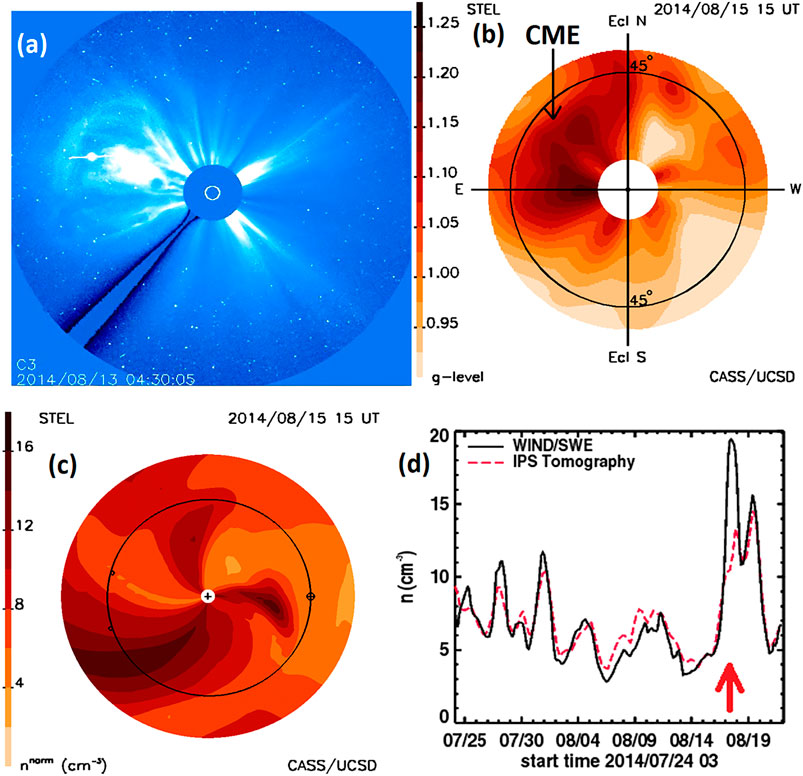
FIGURE 1. (a) A CME is observed erupting from the Sun in LASCO images beginning on August 12, 2014, at ∼21:30 UT. (b) This same CME is depicted as reconstructed in the UCSD tomography g-level 2½ days later when the CME has reached beyond 45° elongation. (c) A reconstructed ecliptic cut of density for the same time period as (b) shows the backside CME to the east of the Sun–Earth line as a large spiral-like structure. Additionally, a dense CME-like structure has nearly reached the Earth’s position to the right of the image. (d) Density time series for a one-month interval during this period from the NASA Wind spacecraft (black line) and the 3-D reconstructed density (red dashed line) showing the time of the CME onset at Earth (red arrow) about 4 days following their solar eruption.

Summaries of how the iterative time-dependent tomography reconstructs the inner heliosphere are found in Jackson and Hick (2005); Hick and Jackson (2004); Jackson et al. (2001); Jackson et al. (2003); Jackson et al. (2006); Jackson et al. (2007); Jackson et al. (2008a); Jackson et al. (2009); and Jackson et al. (2011a). A comprehensive mathematical treatment of the time-dependent IPS and Thomson-scattering tomography is given in Jackson et al. (2008b). The analysis assumes starting values for velocity and density at an inner boundary “source surface”. From these initial values, a best fit is reached through iteration. When the LOS integrations through the 3-D solar wind volumes at large solar distances differ from the overall observations, the source-surface values that have been traced back by the outward velocity propagation are inverted tomographically using a least-squares fitting procedure to provide values that reduce the deviations along the LOS. This produces the next set of source-surface values over time that are propagated outward and used to provide new 3-D volumes, and new corrections to the source surface. Iterations are monitored and show that the procedure quickly converges after a few steps. Confirmation of how well the IPS tomography operates with respect to other analysis available at the CCMC is given for seven-month intervals in both 2006 and 2007 by Jian et al. (2015); Jian et al. (2016). Magnetic field extrapolations using the IPS kinematic modeling are presented in a comprehensive effort using over 10 years of data (2006–2016) in Jackson et al. (2016b) and to forecast magnetic field GSM Bz over 11 years of data (2006–2017) in Jackson et al. (2019). Even more recently, the IPS-driven ENLIL programming is explored and contrasted with other models for use in forecasting ICMEs over 6-month periods of data in 2014 and 2016 (Gonzi et al., 2020).

For the IPS tomography, both density and velocity solar wind models are iterated to fit observed values. In this analysis, the small-scale electron density variations (δNe) that provide g-level are converted from density by Eq. 1.

$\delta Ne\approx A{R}^{\alpha }{N}^{\beta }(1)$

where A is a constant, R is the radial distance from the Sun, N is the proton bulk density, and the power β is set in our analysis to fit in situ proton bulk density at Earth (where electrons are held in neutral equilibrium, primarily with protons and helium atoms in the solar wind). Values of α and β were developed in our analysis of the large variation of bulk proton density observed in the Bastille Day CME event from year 2000 compared with the Advanced Composition Explorer (ACE) spacecraft (Stone et al., 1998) Solar Wind Electron Proton Alpha Monitor (SWEPAM) (McComas et al., 1998), level zero data. These have not been changed since that time but are checked periodically to determine how well they fit current data sets. Constant A is removed by the way g-level is defined. The value of AR^αN^β is integrated along the LOS and weighted using the IPS thin scattering theory developed by Young (1971). This LOS weighting is shown for different radio frequencies, and radio source sizes including that of the ISEE 327 MHz observations in Figure 2. The weighting, which does not include the different LOS changes in g-level, is essentially the same for any direction in the sky but differs according to the frequency of the radio signal and the size of the radio source. In practice, the radio frequency for the observation is well-known, but the source size that varies with this frequency is often poorly determined and can have an irregular shape that depends on the flow of the solar wind across it.

FIGURE 2

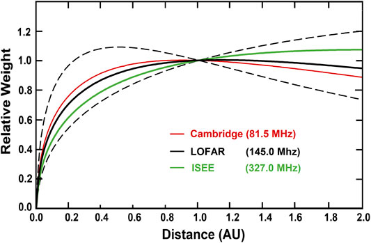
FIGURE 2. The IPS LOS weighting distribution for different observing frequencies and assumed source sizes relative to distance along the LOS from Earth in the direction to the source. The weights are “normalized” at 1 AU and do not include the different scattering amounts along the LOS including those from the changing amount of scatterers with distance from the Sun. Cambridge, LOFAR, and ISEE source sizes are given at 0.3, 0.2, and 0.1 arcsec, respectively. Dashed lines lower and upper are source sizes at the LOFAR frequency for 0.1 and 0.3 arcsec source sizes, respectively. Frequency and source size need to be accommodated for each radio source observed.

The IPS velocity observations are usually presented relative to the integrated value perpendicular to the LOS. The actual solar wind speed varies with distance along the LOS relative to the radial, and in integration along the LOS this deviation of the solar wind propagation relative to the radial direction is taken into account. In addition, the velocity weighting along the LOS is usually assumed to be the same as that for small-scale electron density scattering as given in Eq. 1. When both velocity and IPS g-level are available, they are simultaneously iterated to provide best fits to the g-level values that give density variations along the LOS to show density structure, but these also provide weighting along the LOS that give better velocity fits. Likewise, the velocity reconstructions provide more accurate traceback locations for the source surface density spatial and temporal initial positions to provide better fits for the g-level observations.

The 3-D reconstructions provide an analysis of the shape of the structures tracked without assuming a predefined shape for them. To indicate how these single-site perspective views using the IPS analysis provide an iterative solution to do this, we present the analysis of small packets of plasma particles in Figure 3B. Outward-flowing plasma within the inner heliosphere moves nearly radially outward from the Sun, and the range of different perspectives resulting from this motion iteratively provides the LOS differentiation. This figure illustrates the motion and structure brightness difference from ever-expanding 1° outward-flowing solar wind plasma (group #1 at 20° and group #2 at 90° are highlighted). Here, an IPS LOS to different distant sources sees plasma present in the two outflows, but these appear extremely different to the observer situated at 1 AU. Both 1° flows are assumed to have a value of 5 e⁻ cm⁻³ at 1 AU with an r⁻² density fall-off with distance from the Sun, as is present in constant-flowing outward solar wind plasma. Group #1 plasma in the near 1° flow are outward-moving at a constant speed of 400 km s⁻¹, as is typical of the background solar wind or a slow CME. The intersection of this solar wind flow is tracked in position angle at the outward moving speed of this 1° flow to ever greater distances from the Sun (depicted on the Figure 3B abscissa) by the IPS LOS view to different distant radio sources. As shown in Figure 3B, the fractional g-level contribution of the Group #1 plasma increases gradually as the material moves outward. The intersected Group #2 electrons of the more distant solar wind falls off significantly in fractional g-level response as the LOS moves outward. In addition, the plasma in this distant 1° flow would have had to undergo an unphysical acceleration to extreme speeds over this time interval as shown in Figure 3B (green dashed line) to match the motion of the Group 1 plasma. By modeling solar wind flow such that both mass and mass flux are conserved, the distant unrealistic solution to structure flow is quickly eliminated. This plus the greatly different fractional response of the ever-expanding plasma volume along the LOS provides a differentiation of the LOS plasma location using the iterative 3-D reconstruction analysis.

FIGURE 3

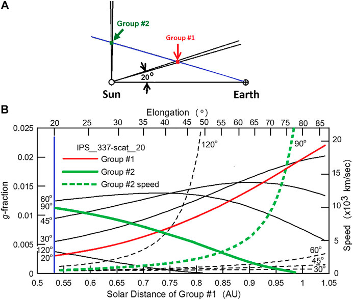
FIGURE 3. (A) Different groups of plasma, one at 20° and one at 90° angular distance from the Sun–Earth line. Both groups move outward at a constant speed of 400 km s⁻¹. (B) Fractional response of IPS g-level (left ordinate) for different groups of electrons moving outward at a speed of 400 km s⁻¹. The Group #1 plasma at 20° (red) and the Group #2 plasma at 90° (green) are highlighted. The Group #1 plasma is tracked and moves outward linearly (lower abscissa) at a constant speed (400 km s⁻¹) and is also shown progressing outward in elongation (upper abscissa). Group #1 electrons for the volume packet (solid red line) provide an ever-increasing fractional percentage of the g-level response. Group #2 electrons that are viewed along the same LOS as those of Group #1 (solid green line) produce an ever-decreasing fraction of the LOS g-level response. Dashed lines show the geometrical speed (right ordinate) that must be present for different groups relative to Group #1 that is tracked outward at constant speed.

The Thomson scattering 3-D reconstruction with views from a single point in space operates in a similar way. This 3-D reconstruction uses well-established electron Thomson-scattering theory (Billings, 1966) to provide its brightness response, and as shown in Figure 4, the LOS response to Thomson-scattered light from electrons is significantly different from that of the IPS shown in Figure 2. Here, each LOS peaks at the closest point to the Sun, and at elongations greater than 90° this is the location of the observer. Polarization brightness (pB) observations that were used in Helios spacecraft photometer 3-D reconstructions (Jackson et al., 2011a) and that are likely to be used in the Polarimeter to Unify the Corona and Heliosphere (PUNCH) observations are more strongly peaked than those shown for Thomson-scattered brightness (B). SMEI only used brightness in its 3-D reconstructions. A depiction of how single-site perspective views using the Thomson-scattering analysis provide an iterative solution to the LOS response by tracking structures outward from the Sun is illustrated in Figure 5. Again, as for the IPS, outward-flowing plasma within the inner heliosphere is shown moving outward radially from the Sun, and the range of different perspectives resulting from this motion provides the LOS differentiation. Figure 5A illustrates the motion and structure brightness and polarization brightness differences from two 1° outflows of solar wind plasma. Here, however, a one-degree widening FOV from Earth (expanding lines in Figure 5A) sees electrons present in the two identical 1° wide outflows centered on the Sun, but these appear extremely different to the observer situated at 1 AU. Both 1° flows have a 5-electron density r⁻² fall-off relative to 1 AU with distance from the Sun, and again Group #1 electrons in the near 1° flow are outward-moving at a constant speed of 400 km s⁻¹. As in Figure 3, the intersection of this solar wind flow is tracked in position angle at the outward moving speed of this 1° flow to ever greater distances from the Sun (depicted on Figure 5B abscissa) by the one-degree FOV. As shown in Figure 5B, the brightness of the Group #1 electrons (given in S10 units for the 1°-wide intersected flow) decreases as the material gets closer to the Earth. The 1° intersected Group #2 electron flow of the more distant solar wind falls off with a more extreme brightness decrease. In addition, as for the IPS the electrons in this distant flow would have had to undergo an unphysical acceleration to extreme speeds (as shown by the dashed increasing line) over this time interval to match the motion of the Group #1 electrons. Dotted decreasing lines with distance depict pB for both groups. The Group #1 pB decrease must also fit the observed structure motion, giving even more confirming information about its LOS location and eliminating any duality of the pB value relative to the point of closest approach of the LOS to the Sun. By modeling solar wind flow such that both mass and mass flux are conserved, the distant unrealistic solution to structure flow is quickly eliminated, and this plus the more extreme fall-off of the distant flow provides the basis of 3-D reconstructions using Thomson-scattering brightness.

FIGURE 4

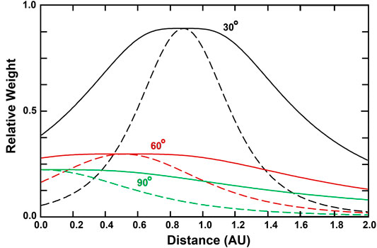
FIGURE 4. Relative Thomson-scattering LOS brightness weighting from the distance of the observer (in AU) at three different solar elongations. For each elongation labeled, two curves are shown; solid lines are B, dashed lines are pB. Amplitude peaks at small elongations have more weight than those at large elongations because electrons in a one-degree column are closer to the Sun at the same distance from the observer.

FIGURE 5

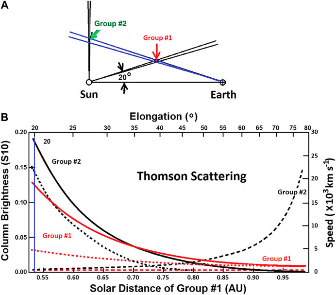
FIGURE 5. (A) The intersection of a 1° outflow of electrons near the Earth (Group #1) along the same one degree opening angle LOS (blue) as one more distant (Group #2) travels a shorter distance outward from the Sun over the same amount of time. (B) Group #1 electrons with a constant speed of 400 km s⁻¹ are shown (right ordinate), as well as the necessary increasing speed of the more distant electrons of Group #2) in order that they have the same angular extent of those in the near Group #1. Group #2 electrons must therefore be different material than what was viewed earlier. Additionally, over this same angular extent, the nearer electron outflow decreases far less in surface B or pB over the same distance (lower abscissa) or elongation (upper abscissa) than the more distant electron outflow.

We note that the above depictions for both the IPS and Thomson scattering are only approximations because outward flow is not uniform over the whole sky, and neither is the density. However, this nonuniformity provides a trackable structure and is used and fit iteratively in the 3-D reconstructions. However, we must remember, both constant and radial outflow are only approximations to actual solar wind conditions. In the UCSD kinematic model, constant flow is modified by mass and mass flux conservation, but only assuming radial outflow. It is well known that other factors can change solar wind flow and enhance plasma density at different locations in the solar wind. These additional factors include solar wind acceleration with distance from the Sun, shock processes, and magnetic fields that interact and modify the solar wind plasma direction and speed. These can be only accommodated in the UCSD 3-D reconstructions by including a better physical model than just radial mass and mass flux conservation. It is for this reason that we include a 3-D MHD kernel as a basis for determining the global solar wind propagation direction and speed as a refinement to our iterative technique.

3-D Reconstructions With an ENLIL Kernel

Numerical solar wind models based on MHD equations are currently the only self-consistent mathematical descriptions capable of bridging many AU outward from the solar surface to well beyond Earth’s orbit. Although MHD is only an approximation to actual plasma behavior, these models have successfully simulated many important space plasma processes and they are utilized by many groups around the world. Several different groups operating MHD analyses have employed the IPS time-dependent tomography boundaries to drive their modeling or have used this IPS modeling to verify their models. These groups include 1) the University of Alabama, Huntsville (UAH) (Kim et al., 2012; Kim et al., 2014; Pogorelov et al., 2012; Yu et al., 2012) who have devised the Multi-Scale FLUid-Kinetic Simulation Suite (MS-FLUKSS) 3-D MHD model; 2) the Naval Research Laboratory group using a model now termed H3D-MHD (Wu et al., 2007; Yu et al., 2015); 3) the University of Michigan group who have developed the BATS-R-US MHD model using the Solar Corona (SC) and Inner Heliosphere (IH) components of the Space Weather Modeling Framework (SWMF) (Meng, 2013; Manchester, 2017; Sachdeva et al., 2019); and; 4) finally, UCSD which has a long-term association with the ENLIL 3-D MHD model and has explored using the IPS boundaries to drive ENLIL since the mid-2000s (Odstrcil et al., 2005b; Odstrcil et al., 2007; Odstrcil et al., 2008; Jackson et al., 2010a; Jackson et al., 2015; Yu et al., 2015).

ENLIL is based on the ideal 3-D MHD description, with two additional continuity equations for tracking the injected CME material and the magnetic field polarity (see Odstrcil and Pizzo, 1999b). Solar wind 3-D MHD modeling often uses photospheric magnetic-field observations (e.g., see Arge and Pizzo, 2000; Arge et al., 2003) and approximates solar wind plasma parameters from these (velocity, density, and temperature) as boundary conditions at the base of the heliosphere and extrapolates these outward. Boundary conditions of transient events, especially velocity and density, are difficult to extract from near-Sun observations and are either “best-guess” approximations to the sources of energy that eject plasma from the Sun or fits to coronagraph data showing the outward speeds of fast-moving structures (CME cone model inputs; Odstrcil and Pizzo, 1999a; Odstrcil et al., 2004; Odstrcil et al., 2005a; Luhmann et al., 2010). Rapidly varying transient CME magnetic-field direct measurements are essentially nonexistent; usually only general background fields are mapped.

The ENLIL 3-D MHD program is exploited by space weather groups for forecasting heliospheric plasma features in advance of their Earth arrival partly because this program is transportable to their institutions. At the KSWC, Jeju, South Korea, this system was operated alongside the UCSD IPS kinematic tomography, which was then modified for use to drive ENLIL in near real time using ISEE IPS data. This system has operated since 2014 by the KSWC in near real time (Figure 6). For the IPS-driven 3-D MHD heliospheric modeling, UCSD has prepared their boundaries, including those for the magnetic field, at the height and in the coordinate system (RTN—Radial Tangential, Normal, or Inertial Heliographic—IHG) required by each model. For some of the modeling, these boundaries have been left on UCSD servers to be employed in each 3-D MHD modeling effort. In recent work using these boundaries (Figure 6, and as described in Yu et al., 2015 or Jackson et al., 2015), the UCSD kinematic model reproduces the in situ record well at the resolutions commensurate with the current IPS data from ISEE. The 3-D MHD models also reproduce the in situ record well using these boundaries.

FIGURE 6

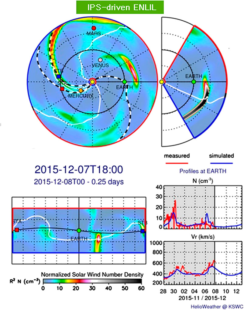
FIGURE 6. ENLIL 3-D MHD density modeling driven by a UCSD IPS tomography-supplied inner boundary at 21.5 Rs, as provided at the KSWC. The 3-D MHD model sample obtained from http://www.spaceweather.go.kr/models/ipsbdenlil is compared with hour-averaged ACE density and velocity data from 28 November to December 07, 2015 and is depicted in the volumetric data at 2015/12/07 18 UT. Once IPS data become available (at 18:00 UT), these analyses are projected 5 days into the future. The black and white dashed lines in the ecliptic cut show the projections of the 3-D field line trace from Earth, STEREO A, and STEREO B at the time of the observation.

An even more significant advance modifies these analyses so that the 3-D MHD modeling can be updated and fit to the IPS observations as structures move outward in the solar wind. This allows observations to update the location of heliospheric structures during their outward propagation such that mid-course corrections can be applied to changing plasma conditions. The ENLIL modeling now provides this advance as a kernel in the UCSD 3-D reconstruction tomography so that it replaces the current kinematic model (Figure 7). In these modeling efforts, we now operate both the kinematic modeling and ENLIL on the same 64-node computer system. ENLIL has been constructed using Fortran MPI and can operate on nodes with different multiples of two; the IPS tomography to date has used only single-string Fortran processing with an IDL system used to output data products. In these initial modeling efforts and for checks, we use a source surface from the kinematic modeling to begin the iterative 3-D reconstructions for the zeroth iteration of the sequence. This enables a kinematic model analysis of the same IPS data set along with IPS-driven modeling at the beginning of the sequence, thus allowing tests to be performed on all three system types at once that are used for checks and updates. The way that this is accomplished using the ENLIL modeling is shown in the Figure 7 flow diagram. Here, the UCSD kinematic model first provides a full time-dependent 3-D reconstruction of the inner heliosphere. This allows the UCSD IDL visualizations of the inner heliosphere as well as time-dependent ENLIL boundary values extracted from these volumes in velocity, density, and three-component magnetic fields at 21.5 Rs. The ENLIL model is then run using these boundaries to provide an IPS-driven ENLIL model, which provides volumetric data in 3-component velocities, 3-component fields, density, and temperature that is used for plots from the ENLIL run. This ENLIL run provides these same time-dependent volumetric data variables up to 3 AU for use in the IPS iterative tomography. A translator FORTRAN program interpolates these volumetric data from ENLIL as multiple time-dependent boundaries for use as needed in the IPS 3-D reconstruction program. These volumetric data are then returned to the UCSD iterative 3-D reconstruction program where the ENLIL 3-component velocity time-dependent matrix then provides solar surface traceback instructions (see “IPS and Thomson Scattering”) for its own use. Iterations of this proceed with the UCSD programming providing renewed output boundaries for ENLIL and ENLIL-produced renewed volumetric data for the tomography. So far, we have found that beginning with a completely converged kinematic model as a start, only about three iterations are required for the iterative ENLIL model to produce consistent results. It takes less than 3 h to complete three iterations on our new UCSD 64-core AMD processor using only 16 cores. At the end of this process, a full UCSD run of its volumetric data as well as that from ENLIL is output and displayed to check consistency between the kinematic model results, and the two versions of ENLIL run with the same IPS inputs and in situ solar wind data sets. These systems have been tested with archival data sets but are also operated in near real time with a 6-h cadence using ISEE IPS data and are displayed on the UCSD web pages under https://ips.ucsd.edu and compared with in situ data available from NOAA, generally from the ACE spacecraft. The real-time display allows checks of all three systems in order to test them under varying input conditions relative to in situ data sets. Figure 8 shows an archival data set comparison using ISEE IPS data and Wind spacecraft in situ measurements. In this example, the iterative ENLIL model clearly shows an advantage in providing a better-resolved dense feature that compares well with Wind in situ density values on September 10, 2011. Even other large density spikes in the in situ sequence on September 2 and September 17 provide a more consistent match between the iterated ENLIL values and Wind. Near real-time comparisons with ACE at current times provide more mixed results, and one of these examples is shown in Figure 9. The sequence of images was taken from the UCSD websites shown on the figure and shows a density time series in comparison with NOAA-provided ACE hour-averages, including a Pearson’s R correlation (R = 0.953) of the density data set up to the time the observational data were available shown as a dashed vertical line. The analysis beyond this has been extended for another 4 days following the run time and shows density decreasing somewhat following the peak after the time the data were obtained. The density did dip by a few particles cm⁻² following this to another peak nearly as high from July 31–August 1. Additional imagery includes a density ecliptic cut, a meridional density cut through Earth, a density synoptic map at 1 AU, a velocity ecliptic cut, and a velocity meridional cut through Earth. The bottom analysis shows the exact same sequence of images in the ENLIL format with the exception of the time series data, which was presented from the third iteration of the 3-D reconstruction model from which the boundary data was used for the final ENLIL imagery shown. This time series has a Pearson’s R correlation of R = 0.808 for its in situ comparison. This additional imagery as well as these is also archived and available for viewing on the two websites presented in Figure 9.

FIGURE 7

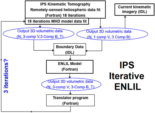
FIGURE 7. The Iterative IPS-ENLIL process depicted as a flow diagram. The UCSD kinematic tomography begins the process and converges from these inputs after three iterations. A “translator” program converts the ENLIL output coordinate system 3-D files over time to those used by the IPS tomography.

FIGURE 8

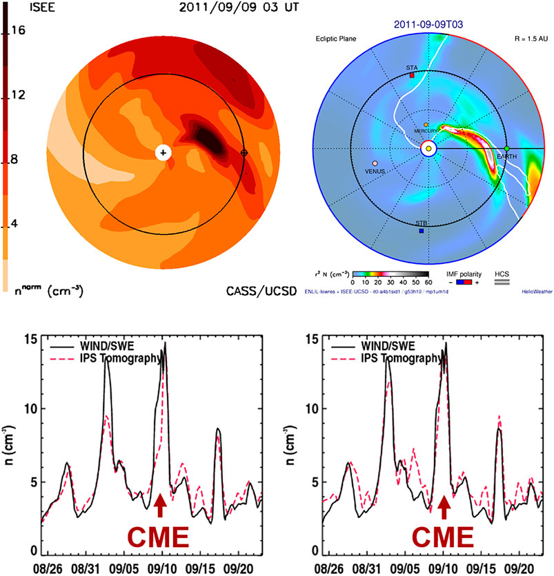
FIGURE 8. Comparison of the density derived from the iterated kinematic model (left) and the iterated model using ENLIL as a kernel (right) in the UCSD tomography. The ecliptic cuts (top) show the modeling for a CME in 2011 from a tomography-supplied inner boundary at 21.5 Rs. Two bottom plots show the comparison of the kinematic model and the ENLIL model for Carrington rotation 2114 with Wind in situ density data that includes this CME. Pearson’s R correlations for the overall density time series kinematic and ENLIL analyses are 0.92, and 0.95, respectively.

FIGURE 9

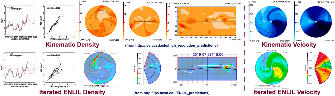
FIGURE 9. (top) Real-time analyses of density and velocity for the IPS kinematic modeling using the ISEE IPS values on July 28, 2019, at 15 UT. (bottom) A third iteration of the 3-D MHD iterative ENLIL model provides similar imagery depicted for this period.

These are encouraging results using both the kinematic modeling or the ENLIL systems, but nevertheless they only show general results in low resolution that provide analyses with a cadence of about half a day from archived data and somewhat less than this used in forecast mode as in Figure 6 or Figure 9. While these analyses provide interesting confirmation of CME structure and density, especially where the IPS data LOS are numerous (near Earth), they provide less information globally, i.e., at non-Earth deep-space locations. As time-dependent fits to heliospheric data, and with confirmation detailed daily by comparison with in situ measurements, these analyses are unique. They are also prone to the idiosyncrasies of data fits and their statistical properties, which provides excellent results only part of the time. With relatively few parameters to fit in the 3-D reconstruction procedures, improvements can generally be made in the prediction by using different data sets and adjusting the parameters to make better fits for specific examples. For the IPS, for instance, the relationship of scintillation level to bulk density shown in, Eq. 1, is one of the only parameters possible to adjust. For the iterated ENLIL programming, the ratio of specific heats, and the heating of various plasma structures is essentially unknown; these two parameters can be adjusted to make better fits most of the time and to this date have not been thoroughly explored. For the ENLIL iterative analysis, more iterations do not seem to improve the results substantially for the examples studied. For ENLIL, there is also a matter of resolution whereby the smoothing used in the 3-D reconstruction procedure cannot adequately distinguish the fine details of shocked plasma density.

For Earth onset plasma forecasting, these analyses still only provide low-resolution state-of-the-art temporal CME measurements with a sparse data set, and the obvious solution is to simply provide more and better-quality data. Additionally, as stated previously, current IPS analyses can miss some of the fastest transient structures simply because they are not observed by a single longitude observational facility. Thus, we now describe a way forward for these same analyses that can be used to provide better-resolved and more secure results from a variety of different techniques.

Advanced Techniques and Summary

As long as space research continues, it will always be important to provide better and more refined analyses globally of this medium through remote-sensing techniques. Such techniques enable an understanding of structures surrounding those that can be measured in situ, and although these measurements can be more precise and obtained at higher cadences, there are simply not enough of them or the resources to provide them throughout space to fill in all the locations of interest. Furthermore, the physics of how solar wind structures are accelerated and interact is still only in its infancy as the main premises of Parker Solar Probe (PSP) and Solar Orbiter amply demonstrate. We expect our analyses to fill in the gaps between in situ measurements where possible and to provide more continuous representation of the spotty global information currently available as well as a better understanding behind the physical processes that create solar wind outflow and their interactions.

Another benefit for forecasting is that the 3-D reconstruction analyses do not require coronagraph or heliospheric imager inputs to provide their predictions to map oncoming CMEs (see, e.g., Jackson et al., 2015). This is good from the standpoint of an autonomous forecast system especially using a 3-D MHD kernel, since all can be done without human intervention except for maintenance of the systems that provide the data and its modeling. There are several ways to remedy the lack of remote sensing data readily available, and for IPS this is by providing more IPS sites around the globe that can input to the remote sensing observations so that there are fewer data gaps and more available data. Over the years, the UCSD 3-D reconstruction analysis has been operated using single instrument data to provide 3-D structure analyses. These include 1) data from the Cambridge, England, array from the year 1979 (Jackson et al., 1998); 2) data from ISEE (Bisi et al., 2008; Bisi et al., 2009a; Bisi et al., 2010b; Jackson et al., 2003; Jackson et al., 2010b; Jackson et al., 2011a; Jackson et al., 2013); 3) data from the Ooty, India, array (Bisi et al., 2009b; Manoharan, 2010); 4) data from EISCAT in northern Europe (Bisi et al., 2010a; Fallows et al., 2007a; Fallows et al., 2007b); 5) data from the Mexican Array Telescope (Chang et al., 2016); and 6) data from the Pushchino, Russia, Big Scanning Array (BSA) (Jackson et al., 2016a).

In 2016, the Worldwide Interplanetary Scintillation Stations (WIPSS) Network (Bisi et al., 2016a; Bisi et al., 2016b; Bisi et al., 2016c; Jackson et al., 2016c) concept was initiated to indicate a standard way to provide results from observations of IPS and allow a unified combination of IPS instruments around the world. The UCSD tomography program had earlier been modified to accommodate many different IPS systems, sort their data, and combine their outputs. Although all groups providing IPS observations have overwhelmingly agreed to this concept (e.g., Bisi et al., 2016b; Bisi et al., 2017a; Bisi et al., 2017b; Bisi et al., 2017c; Bisi et al., 2017d; Bisi et al., 2017e; Bisi et al., 2017f; Bisi et al., 2017g; Bisi et al., 2018; Jackson et al., 2016c; Jackson et al., 2017), the idea has been difficult to implement. The greatest success to date has come from those working with data from the LOw Frequency ARray (LOFAR) (Van Haarlem et al., 2013) who have recently provided a wealth of multi-site IPS velocities for use from campaign-mode observations from this European system. In Figures 10 and 11, we show an analysis in 2019 from an ISEE–LOFAR combined data set during the PSP second close solar pass where only ISEE g-level data and LOFAR velocity data were available. Figure 10 provides IPS g-level images as introduced in Figure 1 presented alongside IPS velocity images. The combined ISEE-LOFAR data of modeled velocities show an integration of the velocity signal perpendicular to the LOS that is a best fit to LOFAR observational velocities. The observed g-level and velocity observational values (small round circles) are superimposed on the model within 3 h of the given UT time. The times of the models and observations presented are separated by 6 h and show the bulk of the data sources observed on that day within the 3-h limit of the UT time, at each site. The model times are different because the bulk of the ISEE observed g-levels are obtained approximately 9 h earlier than the velocities from LOFAR (the difference in longitude between the measurements obtained in Japan and Europe). The LOS locations are coded with values that provide the level of the observation and are circled by a dark line if the observation is above the modeled value, and by a light value if below that of the model. Although the model is formed by all lines of sight over a period of 8–10 days from global observations, the LOS are instantaneous and thus only show the source contribution to the volume within the 3-h time limit of the model. The ecliptic plots show the instantaneous global values of the density and velocity that are derived from the heliospheric models of these parameters. These are presented at the time of the IPS LOFAR skymap modeled velocity observations. In Figure 10, PSP is marked as a small black dot to the left of center and above the ecliptic within the white area that marks the region of strong scattering in the skymaps, and as a small white dot within the 3-D-reconstructed ecliptic cuts in the bottom plots. Figure 11 provides time-series plots at Earth centered on the PSP close solar pass that includes the IPS ACE densities and velocities from NOAA as a weighted input and as compared with in situ values in the 3-D reconstructions. Clearly, the Figure 10 velocity analysis is an advancement because at this time of the year no IPS velocities were available at ISEE to provide global observations. Additionally, with a more careful analysis of these data sets, we find that the IPS LOFAR velocity observations at this time allowed the ISEE data to fit the in situ density data better at Earth than the 3-D reconstructions analyzed where no LOFAR velocity observations were added (Jackson et al., 2020a; Jackson et al., 2020b).

FIGURE 10

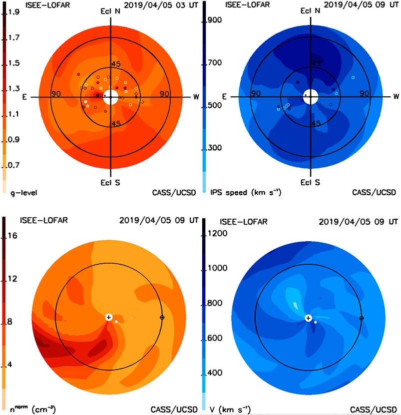
FIGURE 10. (top) IPS skymap observations out to 110° showing the kinematic model analysis using both systems together near the time of the PSP close solar pass. Observations from ISEE (left) and from LOFAR (right) are superimposed on the plot as small circles. The Sun is in the center of the image, and the PSP location is marked as a black dot in the images (bottom) Ecliptic cuts from the same model volumes show the Sun in the center with Earth to the right on its orbit. PSP is located in the images as a white dot superimposed on the ecliptic plot.

FIGURE 11

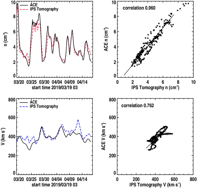
FIGURE 11. (top) Density and (bottom) velocity time series at Earth using ISEE and LOFAR data over Carrington rotation 2215.3 centered on the time period of the PSP second close pass of the Sun.

Other ways to provide the 3-D time-dependent reconstructions globally include measurement of Thomson scattering like those from the Solar Mass Ejection Imager (SMEI). SMEI was a unique instrument designed to provide heliospheric Thomson-scattering observations from Earth to be used in this same way. Launched in January 2003, initially funded by NASA and the Air Force with some NSF support (Jackson et al., 2004). SMEI was shut down after more than eight years of operation in September 2011 (Howard et al., 2013). Some data analysis from SMEI has continued with studies of solar jetting (Yu et al., 2016). The SMEI data still exist, and recently with advent of NASA funding for the Small Explorer Spacecraft PUNCH, there has been an interest in the resurrection of tests of these data sets for its 3-D reconstruction application with this new system.

Our current computer system has been used with existing SMEI data (Figure 12) to provide time series interpolated to 1-h resolutions at Earth, and comparable interpolated time and spatial resolution model analyses. It provides this resolution all the way from the model source surface at 15 Rs from the Sun. This program now can include 1-h ACE or Wind in situ measurements to help normalize the observations at 1 AU. We show the preliminary analysis of this data set for density the May 30, 2003, CME event sequence (Jackson et al., 2008a), shown in Figure 12, which required slightly over 33 h to provide this result on the AMD machine using 14.4% of the 512 Gigabyte memory, and thus this is clearly insufficient as a real-time system at the moment. Figure 13 shows this same event as a volumetric cut through the ecliptic and the north–south ecliptic meridian along the Sun–Earth line at three different times during the event passage. Although nearly all of the global heliosphere can be filled by this iterative tomography technique, here we show only that portion where at least 10 complete LOS provide the 3-D reconstruction in a given resolution element. In this way, the analysis shows that there is ample LOS information to provide a robust reconstruction over the time of the event passage. The SMEI tomography displayed on the UCSD website http://smei.ucsd.edu provides both an ecliptic cut and an Earth meridional cut of these LOS crossing numbers for the low-resolution SMEI data analyses for years 2003–2011 that are archived on this website. This analysis is encouraging, since it implies that with even better programming perhaps using parallel processing, a relatively small computer might allow an even better result with extant SMEI, or STEREO HI data. Of course, we intend that this tomographic system will be regularly employed using observations from PUNCH or UCSD’s own All Sky Heliospheric Imager (ASHI) instrument. The latter is designed specifically for CME and SIR forecasting, as presented to the Space Experiments Review Board for inclusion by the DoD for a Space Test Program flight. As a scientific instrument, this is also very interesting. As an example of this, we note the small peak in density behind the main peak observed in both ACE and Wind in situ measurements on May 30 at ∼9 UT that we suspect may be a reverse shock (see Liu et al., 2017 and references therein) that has just formed and whose extent we can characterize in 3-D as the CME moves outward past the Earth. In the case of the May 30, 2003, CME event sequence, this will mean that we need to use difference volumetric techniques to explore structure evolution relative to the main outward moving solar wind density features.

FIGURE 12

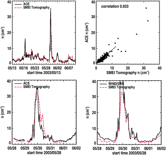
FIGURE 12. SMEI in situ density values plotted with a 1-h cadence. (top) Plotted over the full Carrington rotation 2003 data set that begins on May 13, 2003, relative to ACE Level zero data; (bottom) relative to the same data set plotted from May 28, 2003, to June 2, 2003, centered on the large density peak at the time of the May 30, 2003, CME and (left) relative to the 1-h averaged Wind in situ density measurements.

FIGURE 13

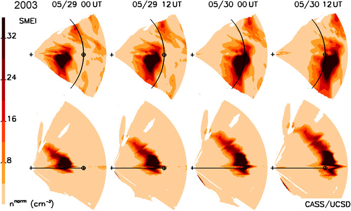
FIGURE 13. SMEI time-dependent ecliptic (top) and meridional (bottom) cuts of the May 30, 2003, CME as it propagates outward past the Earth from which the in situ densities of Figure 12 were obtained. These use the same density color scales as in Figure 1, with enhanced values highlighted above the 5 particle cm⁻³ base.

Conclusion

The preceding text shows how the 3-D reconstructions described can be implemented, combined, and refined to make full use of the planned remote-sensing data imagery that are both ground-based (radio) and available from space-borne instrumentation (Thomson scattered visible light). Utilized in a global 3-D heliospheric system that is refined and used to extend in situ data sets, IPS and/or Thomson-scattering data and its modeling will allow the provision of validated 3-D reconstructions of the inner heliosphere. This can be used to refine current modeling techniques, including time-dependent 3-D MHD as well as IPS analyses of all ground-based systems. Although we show both 3-D reconstruction techniques here for possible future use, only the IPS analyses are immediately at hand to provide this type of forecasting. It is only with great difficulty, expense, and uncertainty that space-borne instrumentation will be able to provide similar and supplemental 3-D analyses. Well-calibrated Thomson-scattering data are not as easy to provide, primarily because the signal is small relative to the other many noise sources present, and imagery can be interpreted simply by approximating (or guessing) the LOS extent present in the imagery. Of course, for 3-D reconstructions both systems can be combined and contrasted as shown to provide the best science and forecasting or both. In any case, the best science, and a most exact 3-D reconstruction definition of the heliosphere, will ultimately lead to the best processes employed to provide this.

Data Availability Statement

The datasets presented in this study can be found in online repositories. The names of the repository/repositories and accession number(s) can be found below: https://ips.ucsd.edu.

Author Contributions

BJ is the primary person responsible for the Iterative Tomography Technique. He and colleagues AB and LC at UCSD helped in the preparation of this article for publication and in the preparation of some of the figures presented. DO at GMU and NASA Goddard is the main person responsible for developing the ENLIL 3-D MHD program used in the article. MB and RF are the main persons responsible for providing and preparing the LOFAR velocity data for use in the 3-D tomography program. MT at ISEE, Japan and his group have prepared the ISEE IPS data for presentation, and have provided these data for use on their FTP website in Japan.

Funding

The work of BJ, AB, and LC acknowledge funding from NASA contracts 80NSSC17K0684, and NNX17AG13G, and AFOSR contract FA9550-19-1-0356 P00001 DEF to the University of California, San Diego. DO acknowledges NASA LWS sub-award 96916956 and MB LWS subcontract RS00963 contract no. 5666 to the University of California, San Diego. MB was also supported by the STFC in-house Research Grant to UKRI STFC RAL Space—Space Physics and Operations Division. The ILT resources have benefitted from the following recent major funding sources: CNRS-INSU, Observatoire de Paris, and Universite d’Orleans, France; BMBF, MIWF-NRW, MPG, Germany; Science Foundation Ireland (SFI), Department of Business, Enterprise and Innovation (DBEI), Ireland; NWO, The Netherlands; The Science and Technology Facilities Council, United Kingdom; and Ministry of Science and Higher Education, Poland.

Conflict of Interest

The authors declare that the research was conducted in the absence of any commercial or financial relationships that could be construed as a potential conflict of interest.

Acknowledgments

The authors wish to thank the many persons responsible for this chapter in Frontiers in Solar and Space Weather. Paul Hick, who provided much of the original work on the IPS and SMEI 3-D reconstruction programming, is greatly appreciated for his many contributions to these studies. This paper is based in part on data obtained with the International LOFAR Telescope (ILT) under project code “LT10_001.” LOFAR (Van Haarlem et al., 2013) is the Low Frequency Array designed and constructed by ASTRON. It has observing, data processing, and data storage facilities in several countries that are owned by various parties (each with their own funding sources) and that are collectively operated by the ILT foundation under a joint scientific policy.

References

Arge, C. N., Odstrcil, D., Pizzo, V. J., and Mayer, L. R. (2003). Improved method for specifying solar wind speed near the Sun. AIP Conf. Proc. 679, 190–193. doi:10.1063/1.1618574

CrossRef Full Text | Google Scholar

Arge, C. N., and Pizzo, V. J. (2000). Improvement in the prediction of solar wind conditions using near-real time solar magnetic field updates. J. Geophys. Res. 105, 10465–10479. doi:10.1029/1999ja000262.

CrossRef Full Text | Google Scholar

Barnes, D. (2020). Remote sensing estimates of CME density in the ecliptic using the STEREO heliospheric imagers. J. Geophys. Res. Space Phys. 125(2), 12–27. doi:10.1029/2019JA027175.

CrossRef Full Text | Google Scholar

Behannon, K. W., Burlaga, L. F., and Hewish, A. (1991). Structure and evolution of compound streams at ≤1 AU. J. Geophys. Res. 96(21), 213. doi:10.1029/91ja02267.

CrossRef Full Text | Google Scholar

Billings, D. E. (1966). A guide to the solar corona. New York, NY: Academic Press, 150.

Google Scholar

Bisi, M. M., Jackson, B. V., Hick, P. P., Buffington, A., and Clover, J. M. (2008). 3D reconstructions of the early november 2004 CDAW geomagnetic storms: preliminary analysis of STELab IPS speed and SMEI density. J. Geophys. Res. Space Phys. 23(113), A00A11. doi:10.1029/2008ja013222

CrossRef Full Text | Google Scholar

Bisi, M. M., Jackson, B. V., Buffington, A., Clover, J. M., Hick, P. P., and Tokumaru, M. (2009a). Low-resolution STELab IPS 3D reconstructions of the whole heliosphere interval and comparison with in-ecliptic solar wind measurements from STEREO and wind instrumentation. Sol. Phys.Sol Phys. 256, 201–217. doi:10.1007/s11207-009-9350-9.

CrossRef Full Text | Google Scholar

Bisi, M. M., Jackson, B. V., Clover, J. M., Manoharan, P. K., Tokumaru, M., Hick, P. P., et al. (2009b). 3-D reconstructions of the early-November 2004 CDAW geomagnetic storms: analysis of Ooty IPS speed and density data. Ann. Geophys. 27, 4479. doi:10.5194/angeo-27-4479-2009.

CrossRef Full Text | Google Scholar

Bisi, M. M., Jackson, B. V., Breen, A. R., Dorrian, G. D., Fallows, R. A., Clover, J. M., et al. (2010a). Three-dimensional (3-D) reconstructions of EISCAT IPS velocity data in the declining phase of solar cycle 23. Sol. Phys. 265, 233–244. doi:10.1007/s11207-010-9594-4.

CrossRef Full Text | Google Scholar

Bisi, M. M., Breen, A. R., Jackson, B. V., Fallows, R. A., Walsh, A. P., Mikić, Z., et al. (2010b). From the Sun to the Earth: the 13 may 2005 coronal mass ejection. Sol. Phys. Sol Phys. 265, 49–127. doi:10.1007/s11207-010-9602-8.

CrossRef Full Text | Google Scholar

Bisi, M. M., Fallows, R. A., Sobey, C., Eftekhari, T., Jensen, E. A., Jackson, B. V., et al. (2016a). “Worldwide interplanetary scintillation (IPS) and heliospheric Faraday rotation plans and progress,” in Oral presentation at the IPSP SANSA space weather research forum, SANSA abstract Hermanus, South Africa, January 20, 2016.

Google Scholar

Bisi, M. M., Jackson, B. V., and Webb, D. F. (2016b). “Remote-Sensing observing techniques for improving space-weather science and forecasting,” in Oral presentation at the 2016 SHINE conference, SHINE abstract Santa Fe, New Mexico, July 15, 2016

Google Scholar

Bisi, M. M., Gonzalez-Esparza, J. A., Aguilar-Rodriguez, E., Chang, T. O., Jackson, B. V., Yu, H.-S., et al. (2016c). “The worldwide interplanetary scintillation (IPS) stations (WIPSS) Network,” ESWW abstract in Presentation at the 13th European space weather week, November 14–18, 2016

Google Scholar

Bisi, M. M., Gonzalez-Esparza, J. A., Jackson, B., Aguilar-Rodriguez, E., Tokumaru, M., Chashei, I., et al. (2017a). “The worldwide interplanetary scintillation (IPS) Stations (WIPSS) Network in support of space-weather science and forecasting,” in Paper presented at Geophysical Research Abstracts, EGU General Assembly, Vienna, Austria, April 23–28, 2017

Google Scholar

Bisi, M. M., Fallows, R. A., Jackson, B. V., Tokumaru, M., Yu, H.-S., and Barnes, D. (2017b). “.The worldwide interplanetary scintillation (IPS) stations (WIPSS) Network: October 2016 campaign—LOFAR and ISEE initial Investigations,” in Paper presented at space weather workshop, NOAA SWW abstract, Broomfield, CO, May 1–5, 2017

Google Scholar

Bisi, M. M., Gonzalez-Esparza, J. A., Jackson, B. V., Aguilar-Rodriguez, E., Tokumaru, M., Chashei, I., et al. (2017c). “The worldwide interplanetary scintillation (IPS) Stations (WIPSS) Network in Support of space-weather science and forecasting,” in Oral presentation at the IAU space weather of the heliosphere conference, IAU abstract, Exeter, UK, July 17–21, 2017

Google Scholar

Bisi, M. M., Fallows, R. A., Jackson, B. V., Tokumaru, M., Yu, H.-S., Morgan, J., et al. (2017d). “The worldwide interplanetary scintillation (IPS) stations (WIPSS) Network October 2016 campaign: LOFAR IPS data analyses,” in Poster presentation at the IAU space weather of the heliosphere conference, IAU abstract, Exeter, UK, July 17–21, 2017

Google Scholar

Bisi, M. M., Webb, D. F., Gonzalez-Esparza, J. A., Jackson, B. V., Chashei, I., Tokumaru, M., et al. (2017e). “The worldwide interplanetary scintillation (IPS) stations (WIPSS) Network as a potential future ISWI instrument,” in Presentation at the UN/US workshop on the International space weather initiative, UN/US abstract, Boston, MA, July 31–August 4, 2017

Google Scholar

Bisi, M. M., Jackson, B. V., Fallows, R. A., Tokumaru, M., Aguilar-Rodriguez, E., Gonzalez-Esparza, A., et al. (2017f). “The worldwide interplanetary scintillation (IPS) Stations (WIPSS) Network: Initial results from the October 2016 space-weather campaign,” in Oral presentation at session 9 at the European space weather week 14, ESWW abstract, Oostende, Belgium, November 27–December, 01, 2017

Google Scholar

Bisi, M. M., Fallows, R. A., Jackson, B. V., Tokumaru, M., Gonzalez-Esparza, A., Morgan, J., et al. (2017g). “The worldwide interplanetary scintillation (IPS) Stations (WIPSS) Network October 2016 observing campaign: initial WIPSS data analyses,” in Presentation SH21A-2648, AGU abstract, AGU Fall Meeting, New Orleans, LA, December 11–15, 2017.

Google Scholar

Bisi, M. M., Jackson, B. V., Fallows, R. A., Chang, O., Tokumaru, M., Aguilar-Rodriguez, E., et al. (2018). “The worldwide interplanetary scintillation (IPS) stations (WIPSS) Network: recent campaign results including LOFAR and steps towards LOFAR for space weather (LOFAR4SW),” in Poster presentation at the 15th European space weather workshop, ESWW abstract Leuven, Belgium, November 5–9, 2018.

Google Scholar

Brueckner, G. E., Howard, R. A., Koomen, M. J., Korendyke, C. M., Michels, D. J., Moses, J. D., et al. (1995). The Large Angle Spectroscopic Coronagraph (LASCO): visible light coronal imaging and spectroscopy. Sol. Phys. 162, 357–402. doi:10.1007/bf00733434.

CrossRef Full Text | Google Scholar

Buffington, A., Morrill, J. S., Hick, P. P., Howard, R. A., Jackson, B. V., and Webb, D. F. (2007). Analysis of the comparative responses of SMEI and LASCO. Proc. SPIE. 6689, 66890B1–66890B6. doi:10.1117/12.734658

CrossRef Full Text | Google Scholar

Chang, O., Jackson, B. V., González-Esparza, A., Yu, H.-S., and Mejia-Ambriz, J. (2016). “Incorporation of MEXART interplanetary scintillation (IPS) data into the UCSD 3-D tomography as part of the worldwide IPS Stations (WIPSS) initiative: enhancing space weather science and forecasting” in Poster presentation, SHINE workshop, Santa Fe, NM, July 11–15.

Google Scholar

Domingo, V., Fleck, B., and Poland, A. I. (1995). The SOHO mission: an overview. Sol. Phys. 162, 1–37. doi:10.1007/bf00733425.

PubMed Abstract | CrossRef Full Text | Google Scholar

Dryer, M., Candelaria, C., Smith, Z. K., Steinolfson, R. S., Smith, E. J., Wolfe, J. H., et al. (1978). Dynamic MHD modeling of the solar wind disturbances during the August 1972 events. J. Geophys. Res. 83, 532–540. doi:10.1029/ja083ia02p00532.

CrossRef Full Text | Google Scholar

Dunn, T., Jackson, B. V., Hick, P. P., Buffington, A., and Zhao, X. P., (2005). Comparative analyses of the CSSS calculation in the UCSD tomographic solar observations. Sol. Phys. 227, 339–353. doi:10.1007/s11207-005-2759-x.

CrossRef Full Text | Google Scholar

Eyles, C. J., Harrison, R. A., Davis, C. J., Waltham, N. R., Shaughnessy, B. M., Mapson-Menard, H. C. A., et al. (2009). The heliospheric imagers onboard the STEREO mission. Sol. Phys. 254, 387–445. doi:10.1007/s11207-008-9299-0.

CrossRef Full Text | Google Scholar

Eyles, C. J., Simnett, G. M., Cooke, M. P., Jackson, B. V., Buffington, A., Hick, P. P., et al. (2003). The solar mass ejection imager (SMEI). Sol. Phys. 217, 319–347. doi:10.1023/b:sola.0000006903.75671.49.

CrossRef Full Text | Google Scholar

Fallows, R. A., Breen, A. R., Bisi, M. M., Jones, R. A., and Dorrian, G. D. (2007b). IPS using EISCAT and MERLIN: extremely-long baseline observations at multiple frequencies. Available at: www.prao.ru/conf/Colloquium/pres/Fallows.ppt (Accessed 2007).

Google Scholar

Fallows, R. A., Breen, A. R., Bisi, M. M., Jones, R. A., and Dorrian, G. D. (2007a). Interplanetary scintillation using EISCAT and MERLIN: extremely long baselines at multiple frequencies. Astronom. Astrophys. Trans. 26(6), 489–500. doi:10.1080/10556790701612197.

CrossRef Full Text | Google Scholar

Feng, X., Ma, X., and Xiang, C. (2015). Data-driven modeling of the solar wind from 1 Rsto 1 AU. J. Geophys. Res. Space Phys. 120, 10159. doi:10.1002/2015JA021911.

CrossRef Full Text | Google Scholar

Gonzi, S., Weinzierl, M., Bocquet, F.-X., Bisi, M. M., Odstrcil, D., Jackson, B. V., et al. (2020). Impact of inner heliospheric boundary conditions on solar wind predictions at Earth. Space Weather. 10, 33–49. doi:10.1029/2020sw002499.

CrossRef Full Text | Google Scholar

Gopalswamy, N., Yashiro, S., Michalek, G., Stenborg, G., Vourlidas, A., Freeland, S., et al. (2009). The SOHO/LASCO CME catalog. Earth Moon Planet. 104, 295–313. doi:10.1007/s11038-008-9282-7.

PubMed Abstract | CrossRef Full Text | Google Scholar

Hayashi, K., Kojima, M., Tokumaru, M., and Fujiki, K. (2003). MHD tomography using interplanetary scintillation measurement. J. Geophys. Res. 108(No. A3), 1102, doi:10.1029/2002JA009567.

CrossRef Full Text | Google Scholar

Hayashi, K., Tokumaru, M., and Fujiki, K. i. (2016). MHD‐IPS analysis of relationship among solar wind density, temperature, and flow speed. J. Geophys. Res. Space Phys. 121, 7367–7384. doi:10.1002/2016JA022750.

CrossRef Full Text | Google Scholar

Hewish, A., and Bravo, S. (1986). The sources of large-scale heliospheric disturbances. Sol. Phys. 106, 185–200. doi:10.1007/bf00161362.

CrossRef Full Text | Google Scholar

Hewish, A., Scott, P. F., and Wills, D. (1964). Interplanetary scintillation of small diameter radio sources. Nature. 203, 1214. doi:10.1038/2031214a0.

CrossRef Full Text | Google Scholar

Hick, P. P., and Jackson, B. V. (2004). Heliospheric tomography: an algorithm for the reconstruction of the 3D solar wind from remote sensing observations. Proc. SPIE. 5171, 287–297. doi:10.1117/12.513122

CrossRef Full Text | Google Scholar

Houminer, Z. (1971). Corotating plasma streams revealed by interplanetary scintillation. Nat. Phys. Sci. 231, 165–167. doi:10.1038/physci231165a0.

CrossRef Full Text | Google Scholar

Howard, R. A., Moses, J. D., Vourlidas, A., Newmark, J. S., Socker, D. G., Plunkett, S. P., et al. (2008). Sun Earth connection coronal and heliospheric investigation (SECCHI). Space Sci. Rev. 136, 67. doi:10.1007/s11214-008-9341-4.

CrossRef Full Text | Google Scholar

Howard, T. A., Bisi, M. M., Buffington, A., Clover, J. M., Cooke, M. P., Eyles, C. J., et al. (2013). The solar mass ejection imager and its heliospheric imaging legacy. Space Sci. Rev. 180, 1, doi:10.1007/s11214-013-9992-7.

CrossRef Full Text | Google Scholar

Iwai, K., Shiota, D., Tokumaru, M., Fujiki, K., Den, M., and Kubo, Y. (2019). Development of a coronal mass ejection arrival time forecasting system using interplanetary scintillation observations. Earth Planets Space. 71(1), 39. doi:10.1186/s40623019-1019-5.

CrossRef Full Text | Google Scholar

Jackson, B. V., and Hick, P. P. (2002). Corotational tomography of heliospheric features using global Thomson scattering data. Sol. Phys. 211, 344. doi:10.1023/a:1022409530466.

CrossRef Full Text | Google Scholar

Jackson, B. V., and Hick, P. P. (2005). “Three-dimensional tomography of interplanetary disturbances, Chapter 17” in Solar and space weather radiophysics, current status and future developments, Astrophysics and space science library. Editors D. E. Gary and C. U. Keller (Dordrecht, The Netherlands: Kluwer Academic Publisher), vol. 314, 355–386.

Google Scholar

Jackson, B. V., Hick, P. L., Kojima, M., and Yokobe, A. (1997). Heliospheric tomography using interplanetary scintillation observations. Phys. Chem. Earth. 22(5), 425. doi:10.1016/s0079-1946(97)00170-5.

PubMed Abstract | CrossRef Full Text | Google Scholar

Jackson, B. V., Hick, P. L., Kojima, M., and Yokobe, A. (1998). Heliospheric tomography using interplanetary scintillation observations 1. Combined Nagoya and Cambridge data’, J. Geophys. Res. 103(12), 049. doi:10.1029/97ja02528.

CrossRef Full Text | Google Scholar

Jackson, B. V., Buffington, A., and Hick, P. P. (2001). “A heliospheric imager for solar orbiter” in Proceedings of the solar encounter: the first solar orbiter workshop, Santa Cruz de Tenerife, Spain, May 14–18, ESA SP-493, 251.

Google Scholar

Jackson, B. V., Hick, P. P., Buffington, A., Kojima, T. M., Fujiki, K., et al. (2003). Time-dependent tomography of hemispheric features using interplanetary scintillation (IPS) remote-sensing observations. Solar Wind Ten 679, 75–78. doi:10.1063/1.1618545

CrossRef Full Text | Google Scholar

Jackson, B. V., Buffington, A., Hick, P. P., Altrock, R. C., Figueroa, S., Holladay, P. E., et al. (2004). The Solar Mass-Ejection Imager (SMEI) Mission. Sol. Phys. 225, 177–207. doi:10.1007/s11207-004-2766-3.

CrossRef Full Text | Google Scholar

Jackson, B. V., Buffington, A., Hick, P. P., Wang, X., and Webb, D. (2006). Preliminary three-dimensional analysis of the heliospheric response to the 28 October 2003 CME using SMEI white-light observations. J. Geophys. Res. 111 (A4), A04S91. doi:10.1029/2004ja010942.

CrossRef Full Text | Google Scholar

Jackson, B. V., Hick, P. P., Buffington, A., Bisi, M. M., Kojima, M., and Tokumaru, M. (2007). “Comparison of the extent and mass of CME events in the interplanetary medium using IPS and SMEI Thomson scattering observations,” in Scattering and scintillation in radio astronomy, astronomical and astrophysical transactions. Editors I. Chashei and V. Shishov (London, UK: Oxford University Press), 477–487.

Google Scholar

Jackson, B. V., Bisi, M. M., Hick, P. P., Buffington, A., Clover, J. M., and Sun, W. (2008a). Solar Mass Ejection Imager 3-D reconstruction of the 27–28 May 2003 coronal mass ejection sequence. J. Geophys. Res. 113, A00A15. doi:10.1029/2008JA013224.

CrossRef Full Text | Google Scholar

Jackson, B. V., Hick, P. P., Buffington, A., Bisi, M. M., Clover, J. M., and Tokumaru, M. (2008b). Solar mass ejection imager (SMEI) and interplanetary scintillation (IPS) 3D-reconstructions of the inner heliosphere. Adv. Geosci. 21, 339–366. doi:10.1142/9789812838209_0025

CrossRef Full Text | Google Scholar

Jackson, B. V., Hick, P. P., Buffington, A., Bisi, M. M., and Clover, J. M. (2009). SMEI direct, 3-D-reconstruction sky maps, and volumetric analyses, and their comparison with SOHO and STEREO observations. Ann. Geophys. 27, 4097. doi:10.5194/angeo-27-4097-2009.

CrossRef Full Text | Google Scholar

Jackson, B. V., Buffington, A., Hick, P. P., Clover, J. M., Bisi, M. M., and Webb, D. F. (2010a). Smei 3D reconstruction of a coronal mass ejection interacting with a corotating solar wind density enhancement: the 2008 April 26 CME. Astrophys. J. 724, 829–834. doi:10.1088/0004-637x/724/2/829.

CrossRef Full Text | Google Scholar

Jackson, B. V., Hick, P. P., Bisi, M. M., Clover, J. M., and Buffington, A. (2010b). Inclusion of in-situ velocity measurements into the UCSD time-dependent tomography to constrain and better-forecast remote-sensing observations. Sol. Phys. 265, 245–256. doi:10.1007/s11207-010-9529-0.

CrossRef Full Text | Google Scholar

Jackson, B. V., Hick, P. P., Buffington, A., Bisi, M. M., Clover, J. M., Tokumaru, M., et al. (2011a). Three-dimensional reconstruction of heliospheric structure using iterative tomography: a review. J. Atmos. Sol. Terr. Phys. 73, 1–9. doi:10.1016/j.jastp.2010.10.007.

CrossRef Full Text | Google Scholar

Jackson, B. V., Hamilton, M. S., Hick, P. P., Buffington, A., Bisi, M. M., Clover, J. M., et al. (2011b). Solar Mass Ejection Imager (SMEI) 3-D reconstruction of density enhancements behind interplanetary shocks: In-situ comparison near Earth and at STEREO. J. Atmos. Sol. Terr. Phys. 73, 1317–1329. doi:10.1016/j.jastp.2010.11.023.

CrossRef Full Text | Google Scholar

Jackson, B. V., Hick, P. P., Buffington, A., Clover, J. M., and Tokumaru, M., (2012a). Forecasting transient heliospheric solar wind parameters at the locations of the inner planets. Adv. Geosci. 30, 93–115. doi:10.1142/9789814405744_0007.

CrossRef Full Text | Google Scholar

Jackson, B. V., Clover, J. M., Hick, P. P., Yu, H.-S., Buffington, A., Bisi, M. M., et al. (2012b). The 3D global forecast of inner heliosphere solar wind parameters from Remotely-sensed IPS data. Maui, Hawaii: NSF SHINE abstract, SHINE, June 24–29, 2012.

Google Scholar

Jackson, B. V., Clover, J. M., Hick, P. P., Buffington, A., Bisi, M. M., and Tokumaru, M. (2013). Inclusion of real-time in-situ measurements into the UCSD timedependenttomography and its use as a forecast algorithm. Sol. Phys. 258, 151–165. doi:10.1007/s11207-012-0102-x.

CrossRef Full Text | Google Scholar

Jackson, B. V., Yu, H.-S., Buffington, A., and Hick, P. P. (2014). The dynamic character of the polar solar wind. Astrophys. J. 793, 54. doi:10.1088/0004-637X/793/1/54.

CrossRef Full Text | Google Scholar

Jackson, B. V., Odstrcil, D., Yu, H.-S., Hick, P. P., Buffington, A., Mejia-Ambriz, J. C., et al. (2015). The UCSD kinematic IPS solar wind boundary and its use in the ENLIL 3-D MHD prediction model. Space Weather. 13, 104–115. doi:10.1002/2014SW001130.

CrossRef Full Text | Google Scholar

Jackson, B. V., Yu, H.-S., Chang, O., Hick, P. P., Buffington, A., Tokumaru, M., et al. (2016a). “Space weather forecasting using remotely-sensed heliospheric IPS data sets from around the world—an inclusion of MEXART and BSA Pushchino data into the UCSD STELab IPS tomography,” in Presentation at the space weather workshop, NOAA SWW abstract, Boulder, CO, April 25–29, 2016.

Google Scholar

Jackson, B. V., Yu, H.-S., Buffington, A., Hick, P. P., Nishimura, N., Nozaki, N., et al. (2016b). Exploration of solar photospheric magnetic field data sets using the UCSD tomography. Space Weather. 14 (12), 1107–1124. doi:10.1002/2016SW001481.

CrossRef Full Text | Google Scholar

Jackson, B. V., Yu, H.-S., Hick, P., Buffington, A., Chang, O., Gonzalez-Esparza, A., et al. (2016c). “Worldwide interplanetary scintillation stations (WIPSS) Use of the UCSD IPS tomography program for space weather forecasting,” in Invited presentation at the KSWC space weather workshop, Jeju, South Korea, KSWC abstract, November 24–27, 2016.

Google Scholar

Jackson, B., Yu, H.-S., Hick, P., Buffington, A., Tokumaru, M., Fujiki, K., et al. (2017). “A world interplanetary scintillation stations (WIPSS) tomography program for space weather forecasting.,” in Invited oral presentation at the 2nd PSTEP international symposium, PSTEP 2 abstract, Kyoto, Japan, March 23–24, 2017.

Google Scholar

Jackson, B. V., Yu, H. S., Buffington, A., Hick, P. P., Tokumaru, M., Fujiki, K., et al. (2019). A daily determination of Bz using the Russell–McPherron effect to forecast geomagnetic activity. Space Weather. 17, 639–652. doi:10.1029/2018SW002098.

CrossRef Full Text | Google Scholar

Jackson, B. V., Hick, P. P., Yu, H. S., Buffington, A., and Odstrcil, D. (2020a). “Global heliospheric remote sensing: a Brief recent history,” in Invited oral presentation at the 4th PSTEP international symposium, PSTEP 4 abstract, Nagoya, Japan, January 27–29, 2020.

Google Scholar

Jackson, B. V., Cota, L., Buffington, A., Tokumaru, M., Bisi, M. M., and Fallows, R. (2020b). “ISEE-LOFAR tomography during the second PSP solar passage,” in Invited virtual oral presentation at the LOFAR4SW user workshop hosted at Warsaw, Poland and the UK, by the LOFAR4SW consortium, LOFAR4SW abstract, Warsaw, Polland, May 13, 2020.

Google Scholar

Jian, L. K., MacNeice, P. J., Taktakishvili, A., Odstrcil, D., Jackson, B., Yu, H.-S., et al. (2015). Validation for solar wind prediction at Earth: comparison of coronal and heliospheric models installed at the CCMC. Space Weather. 13, 316. doi:10.1002/2015SW001174.

CrossRef Full Text | Google Scholar

Jian, L. K., MacNeice, P. J., Mays, M. L., Taktakishvili, A., Odstrcil, D., Jackson, B., et al. (2016). Validation for global solar wind prediction using ulysses comparison: multiple coronal and heliospheric models installed at the community coordinated modeling center. Space Weather. 14 (8), 592–611, doi:10.1002/2016sw001435.

CrossRef Full Text | Google Scholar

Sokolov, M. L., Kucera, T. A., Davila, J. M., St. Cyr, O. C., Guhathakurta, M., and Christian, E. (2008). The STEREO mission: an introduction. Space Sci. Rev. 136, 5–16. doi:10.1007/s11214-007-9277-0.

PubMed Abstract | CrossRef Full Text | Google Scholar

Kim, T. K., Borovikov, S. N., Pogorelov, N. V., Yu, H.-S., Clover, J. M., and Jackson, B. V. (2012). “Time-dependent MHD simulations of the solar wind outflow using interplanetary scintillation observations,” in AIP conference proceedings, 1500, space weather: the space radiation environment, 11th annual international astrophysics conference (CSPAR), Palm Springs, CA, March 19–23. Editors Q. Hu, G. Li, G. P. Zank, and X. Ao, 140–146.

Google Scholar

Kim, T. K., Pogorelov, N. V., Borovikov, S. N., Jackson, B. V., Yu, H.-S., and Tokumaru, M. (2014). MHD heliosphere with boundary conditions from a tomographic reconstruction using interplanetary scintillation data. J. Geophys. Res. Space Phys. 119, 7981. doi:10.1002/2013JA019755.

CrossRef Full Text | Google Scholar

Kojima, M., Asai, K., Hick, P. L., Jackson, B. V., Tokumaru, M., Watanabe, H., et al. (1997). “Solar wind structure at 0.1–1 AU reconstructed from IPS observations using tomography,” in Robotic exploration close to the Sun: scientific basis. Editor S. R. Habbal (New York, NY: AIP Press), 97–103.

Google Scholar

Kojima, M., Tokumaru, M., Watanabe, H., Yokobe, A., Asai, K., Jackson, B. V., et al. (1998). Heliospheric tomography using interplanetary scintillation observations: 2. Latitude and heliocentric distance dependence of solar wind structure at 0.1–1 AU. J. Geophys. Res. 103, 1981. doi:10.1029/97ja02162.

CrossRef Full Text | Google Scholar

Liewer, P. C., De Jong, E. M., Hall, J. R., Howard, R. A., Thompson, W. T., Culhane, J. L., et al. (2009). Stereoscopic analysis of the 19 may 2007 erupting filament. Sol. Phys.Sol Phys. 256, 57–72. doi:10.1007/s11207-009-9363-4.

CrossRef Full Text | Google Scholar

Liu, Y. D., Hu, H., Zhu, B., Luhmann, J. G., and Vourlidas, A., (2017). Structure, propagation, and expansion of a Cme-driven shock in the heliosphere: a revisit of the 2012 July 23 extreme storm. Astrophys. J. 834:158. doi:10.3847/1538-4357/834/2/158.

CrossRef Full Text | Google Scholar

Luhmann, J. G., Ledvina, S. A., Odstrcil, D., Owens, M. J., Zhao, X.-P., Liu, Y., et al. (2010). Cone model-based SEP event calculations for applications to multipoint observations. Adv. Space Res. 46, 1–21. doi:10.1016/j.asr.2010.03.011.

CrossRef Full Text | Google Scholar

Manchester, W. (2017). “The determination of heliospheric disturbances by simulations and observations,” in Poster and oral presentation, SHINE workshop, NSF SHINE abstract, Saint-Sauveur, Canada, July, 23–28, 2017.

PubMed Abstract | Google Scholar

Manoharan, P. K. (2010). Ooty interplanetary scintillation—remote-sensing observations and analysis of coronal mass ejections in the heliosphere. Sol. Phys. 265, 137–157. doi:10.1007/s11207-010-9593-5.

CrossRef Full Text | Google Scholar

McComas, D. J., Bame, S. J., Barker, P., Feldman, W. C., Phillips, J. L., Riley, P., et al. (1998). Solar wind electron proton Alpha monitor (SWEPAM) for the advanced composition explorer. Space Sci. Rev. 86, 563. doi:10.1023/a:1005040232597.

PubMed Abstract | CrossRef Full Text | Google Scholar

Meng, X. (2013). Connecting remote-sensing observations and MHD modeling towards a new generation of space weather prediction tools, proposal to the UCAR NASA LWS program.

Google Scholar

Ogilvie, K. W., and Desch, M. D. (1997). The wind spacecraft and its early scientific results. Adv. Space Res. 20(445), 559–568. doi:10.1016/s0273-1177(97)00439-0.

CrossRef Full Text | Google Scholar

Odstrcil, D., and Pizzo, V. J. (1999a). Three-dimensional propagation of coronal mass ejections (CMEs) in a structured solar wind flow. 1. CME launched within the streamer belt. J. Geophys. Res., 104 (A1), 483–492. doi:10.1029/1999ja900319.

CrossRef Full Text | Google Scholar

Odstrcil, D., and Pizzo, V. J. (1999b). Distortion of the interplanetary magnetic field by three-dimensional propagation of coronal mass ejections in a structured solar wind. J. Geophys. Res. 104(28), 225–228. doi:10.1029/1999ja900319.

CrossRef Full Text | Google Scholar

Odstrcil, D., Riley, P., and Zhao, X. P. (2004). Numerical simulation of the 12 May 1997 interplanetary CME event. J. Geophys. Res. 109, A02116. doi:10.1029/2003JA010135.

CrossRef Full Text | Google Scholar

Odstrcil, D., Pizzo, V. J., and Arge, C. N. (2005a). Propagation of the 12 May 1997 interplanetary coronal mass ejection in evolving solar wind structures. J. Geophys. Res. 110, A02106, doi:10.1029/2004JA010745.

CrossRef Full Text | Google Scholar

Odstrcil, D., Pizzo, V. J., Arge, C. N., Jackson, B. V., and Hick, P. P. (2005b). First results from the 3-D MHD heliospheric simulations driven by the SMEI/IPS observations. Proc. SPIE. 259 (1–2), 297–309. doi:10.1007/s11207-009-9449-z

CrossRef Full Text | Google Scholar

Odstrcil, D., Jackson, B. V., and Hick, P. (2007). “3-D numerical simulations of heliospheric disturbances driven by SMEI/IPS observations,” in Paper presented at SEC space weather week, NOAA SWW abstract, Boulder, CO, April 24–27, 2007.

Google Scholar

Odstrcil, D., Pizzo, V. J., Arge, C. N., Bisi, M. M., Hick, P. P., Jackson, B. V., et al. (2008). Numerical simulations of solar wind disturbances by coupled models. ASP Conf. Ser. Proc. 385, 167–173. doi:10.1007/s11207-015-0685-0

CrossRef Full Text | Google Scholar

Parker, E. N. (1958). Dynamics of the interplanetary gas and magnetic fields. Astrophys. J. 128, 664–676. doi:10.1086/146579.

CrossRef Full Text | Google Scholar

Pogorelov, N., Borovikov, S., Ebert, R., Jackson, B., Kim, T., Linker, J., et al. (2012). “Modeling Heliosheath flow with observational boundary conditions,” in Paper presented at the 39th COSPAR scientific assembly, COSPAR abstract, Mysore, India, July 14–22, 2012.

Google Scholar

Pomoell, J., and Poedts, S. (2018). EUHFORIA: European heliospheric forecasting information asset. J. Space Weather Space Clim. 8, A35. doi:10.1051/swsc/2018020.

PubMed Abstract | CrossRef Full Text | Google Scholar

Riley, P., Lionello, R., Mikić, Z., and Linker, J. (2008). Using global simulations to relate the three‐part structure of coronal mass ejections to in situ signatures. Astrophys. J. 672, 1221. doi:10.1086/523893.

CrossRef Full Text | Google Scholar

Sachedeva, N., van der Holst, B., Manchester, W. B., Toth, G., Chen, Y., Lloveras, D. G., et al. , (2019). Validation of the Alfvén Wave Solar Atmosphere Model (AWSoM) with Observations from the Low Corona to 1 au. Astrophs. J. 887, 83. doi:10.3847/1538-4357/ab4f5e.

CrossRef Full Text | Google Scholar

Shen, F., Shen, C., Zhang, J., Hess, P., Wang, Y., Feng, X., et al. (2014). Evolution of the 12 July 2012 CME from the Sun to the Earth: Data-constrained three-dimensional MHD simulations. J. Geophys. Res. Space Phys. 119, 7128–7141. doi:10.1002/2014JA020365.

CrossRef Full Text | Google Scholar

Shiota, D., and Kataoka, R., (2016). Magnetohydrodynamic simulation of interplanetary propagation of multiple coronal mass ejections with internal magnetic flux rope (SUSANOO-CME). Space Weather. 14, 56–75. doi:10.1002/2015SW001308.

CrossRef Full Text | Google Scholar

Steinolfson, R. S., Dryer, M., and Nakagawa, Y., (1975). Numerical MHD simulation of interplanetary shock pairs. J. Geophys. Res. 80, 1223–1231. doi:10.1029/ja080i010p01223.

CrossRef Full Text | Google Scholar

Stone, E. C., Frandsen, A. M., Mewaldt, R. A., Christian, E. R., Margolies, D., Ormes, J. F., et al. (1998). The advanced composition explorer. Space Sci. Rev. 86, 1. doi:10.1023/a:1005082526237.

CrossRef Full Text | Google Scholar

Tokumaru, M., Kojima, M., Fujiki, K. i., Yamashita, M., and Jackson, B. V. (2007). The source and propagation of the interplanetary disturbance associated with the full-halo coronal mass ejection on 28 October 2003. J. Geophys. Res. 112, 39. doi:10.1029/2006JA012043.

CrossRef Full Text

Tokumaru, M., Kojima, M., Fujiki, K., Maruyama, K., Maruyama, Y., Ito, H., et al. (2011). A newly developed UHF radiotelescope for interplanetary scintillation observations: solar wind imaging facility. Radio Sci. 46, RS0F02. doi:10.1029/2011RS004694.

CrossRef Full Text | Google Scholar

Van Harlem, M. P., Wise, M. W., Gunst, A. W., Heald, G., McKean, J. P., Hessels, J. W., et al. (2013). LOFAR: the low-frequency array. Astron. Astrophys. 556, 29. doi:10.1109/iwem.2011.6021486

CrossRef Full Text | Google Scholar

Wang, Y.-M., and Sheeley, N. R. J. (1990). Solar wind speed and coronal flux-tube expansion. Astrophys. J. 355, 726–732. doi:10.1086/168805.

CrossRef Full Text | Google Scholar

Webb, D. F., and Jackson, B. V. (1981). Kinematical analysis of flare spray ejecta observed in the corona. Sol. Phys.Sol Phys. 73, 341–361. doi:10.1007/bf00151686.

CrossRef Full Text | Google Scholar

Wu, C.-C., Fry, C,D., Wu, S.T., Dryer, M., and Liou, K. (2007). Three-dimensional global simulation of interplanetary coronal mass ejection propagation from the Sun to the heliosphere: Solar event of 12 May 1997. J. Geophys. Res. 112, A09104.

Google Scholar

Wu, C. C., Liou, K., Vourlidas, A., Plunkett, S., Dryer, M., Wu, S. T., et al. (2016). Global magnetohydrodynamic simulation of the 15 March 2013 coronal mass ejection event-Interpretation of the 30-80 MeV proton flux, J. Geophys. Res. Space Phys. 121, 56–76. doi:10.1002/2015JA021051.

CrossRef Full Text | Google Scholar

Wu, S. T., Dryer, M., and Han, S. M. (1983). Non-planar MHD model for solar flare-generated disturbances in the heliospheric equatorial plane. Sol. Phys. 84, 395–418. doi:10.1088/0004-637x/784/2/166.

CrossRef Full Text | Google Scholar

Young, A. T. (1971). Interpretation of interplanetary scintillations. Astrophys. J., 168, 543--562.

Google Scholar

Yu, H.-S., Jackson, B. V., Hick, P. P., Buffington, A., Clover, J. M., et al. (2012). “3-D reconstruction of the inner heliosphere from remote-sensing data: a global solar wind boundary that includes CME transient effects,” in AIP conference proceedings, 1500, space weather: the space radiation environment, 11th annual international astrophysics conference (CSPAR), Palm springs, CA, March 19–23. Editors Q. Hu, G. Li, G. P. Zank, and X. Ao, 147–152.

Google Scholar

Yu, H.-S., Jackson, B. V., Buffington, A., and Hick, P. P. (2014). The 3D Analysis of Hinode Polar Jets Using Images From LASCO C2, the STEREO COR 2 Coronagraphs, and the Solar Mass Ejection Imager (SMEI). Astrophys. J., 784, 166. doi:10.1088/0004-637X/784/2/166.

CrossRef Full Text | Google Scholar

Yu, H.-S., Jackson, B. V., Hick, P. P., Buffington, A., Odstrcil, D., Wu, C.-C., et al. (2015). 3D reconstruction of interplanetary scintillation (IPS) remote-sensing data: global solar wind boundaries for driving 3D-MHD models. Sol. Phys.Sol Phys., 290, 2519–2538. doi:10.1007/s11207-015-0685-0.

CrossRef Full Text | Google Scholar

Yu, H.-S., Jackson, B. V., Yang, Y.-H., Chen, N.-H., Buffington, A., and Hick, P. P. (2016). A 17 June 2011 polar jet and its presence in the background solar wind’, J. Geophys. Res. Space Phys. 121, 4985–4997. doi:10.1002/2016JA022503.

CrossRef Full Text | Google Scholar

Zhao, X., and Hoeksema, J. T. (1995). Prediction of the interplanetary magnetic field strength. J. Geophys. Res. 100, 19–33. doi:10.1029/94ja02266.

CrossRef Full Text | Google Scholar