Nested Multi- and Many-Objective Optimization of Team Track Pursuit Cycling

1. Introduction

At the Summer Olympics, team pursuit track cycling is a bicycle racing sport held in velodromes. This sport involves the use of strategies to minimize the overall racing time that a team of cyclists needs. Finding these strategies presents a particularly challenging problem that involves hierarchical dual-level solutions spread over a multi-modal solution space.

Although good strategies can be designed long before the actual competition, it may be necessary to react quickly to changing conditions at the competition venue; for example, a rider in the team has to be replaced due to injury by another rider with various physical properties, such as weight, maximum power output, frontal area, and available amount of energy. As these capabilities and properties influence the team's performance, new racing strategies have to be found within a computationally feasible length of time, for example, within a few hours prior to a race.

Elite cycling has previously been modeled mathematically [1–3] for a single cyclist, where an all-out pacing strategy appears to be optimal. However, when teams cycle, then the solution requires sub-maximal efforts throughout the race [4]. The problem's complexity is the result of several features that arise specific to track-based team cycling. First and foremost, a team of riders who are riding in close formation do so with a lead rider who heads the team and who is then followed by the remaining team members who benefit from the lead rider's slipstream. This slip-streaming effect is an important consideration as it allows riders to conserve energy, as the lead rider typically uses a greater amount of energy. Therefore, teams apply in addition to a pacing strategy a transition strategy, where the lead rider is changed for another, so that the riders may each expend their energy evenly. The problem is further complicated by considering a men's cycling team: contrary to the women's event does the men's event allow for one of the individual riders to remove himself from the race, only requiring that three out of the four riders finish.

In this article, the problem of finding racing strategies is formulated as optimizing two distinct sets of variables. The first set defines the power strategy, i.e., how much power, the lead rider is required to exert in order to ride at the necessary pace. The second set defines the transition strategy, i.e., when during the race a new rider is transitioned to lead. The transition strategy of the riders is affected by the pacing strategy, and an optimal transition strategy for a single pacing strategy may not be optimal for all pacing strategies. Therefore, the minimization of overall time using the pacing strategy depends on having an optimal transition strategy. This dual level optimization results a complex set of solutions because for any given transition strategy it may be impossible to find an optimal pacing strategy and hence only sub-optimal solutions for the overall problem may are created.

1.1. Related Work

Hierarchical programming is concerned with optimizing problems that involve multiple decision makers structured in ordered levels. In hierarchical optimization, the optimization of higher order decision makers influence the decisions made at lower levels [5]. This creates a difficult set of problems as the optimal lower level solution will be different for each upper level solution, creating a situation where multiple trade-off lower level solutions need to be searched, and there is a complex interaction between the upper and lower levels of a problem. This complexity makes it hard to find an optimal solution to the overall problem.

The bilevel optimization problem is a subset of hierarchical problems in which there are two levels of optimization problems. Bard [6] states that bilevel optimization problems commonly appear in real life applications. For example, let us take a practical problem where an optimization task must satisfy a certain set of conditions. The problem itself would be considered the upper level optimization task, while one or more of these conditions can be posed as a lower level optimization task. However, due to the difficulties in solving bilevel problems, these lower level conditions are often represented using approximate methodologies [7].

Hierarchical optimization has been successfully applied to a variety of real life problems. In the realm of single-objective bilevel optimization, there have been some studies of applications, such as in the areas of defence, engineering, energy planning, revenue management, transportation network design and production scheduling problems [8, 9]. Similarly, these same principles have been applied in a study of a single-objective version of our cycling problem [10].

Deb and Sinha [7] have done a comprehensive survey of bilevel multi-objective optimization studies and have found that due to the complexity of this type of problem studies are severely lacking. There has been theoretical research in multiobjective bilevel problems, with Herskovits et al. [11] replacing the Karush-Kuhn-Tucker conditions of the lower level optimization problem as constraints in the upper level problem; however, this is not possible in some real life problems where the lower level problem can be quite complicated. Other studies have handled this type of problem using a nested approach, for example by using an exhaustive search method for the lower level problem [12]. Deb and Sinha [7] present an algorithm for solving bilevel problems using NSGAII to solve both levels of the problem, which were found to be generic, being able to be used on a range of different problems. We build on this work, adapting other multi-objective algorithms to be suitable for use in hierarchical problems in our framework.

In general, iterative heuristic algorithms such as local search, simulated annealing, evolutionary algorithms, and ant colony optimization have proven to be successful problem solvers in a wide range of domains [13]. In this particular article, we will employ the so-called evolutionary algorithms, however, it it important to note that other iterative optimization approaches can be used as well. Evolutionary algorithms form a sub-class of bio-inspired algorithms, who mimic some fundamental aspects of the neo-Darwinian evolutionary process. They simultaneously search with a population of candidate solutions and associate an objective score as a fitness value for each one. The algorithms then select among the population to favor those solutions that are more fit. The next generation (i.e., a new population as a step in the overall evolution) consists of replicates of the fitter solutions that have been genetically mutated and crossed over in a biological metaphor: the decision variables were perturbed such that they inherit characters of their parents, as well as change in random ways.

Regarding optimization in the domain of track cycling, Wagner et al. [4, 14] described a model for the women's team pursuit problem, where three riders form a team, and where race time was minimized as the sole optimization objective. The major point of difference with our problem is that the men's teams consist of four riders (as mentioned above), and of these only three need to reach the finish of the race. Furthermore, the men's event is competed over a longer distance of 4000 m, consisting of 16 laps of the velodrome, compared with the women's which is run over 3000 m (12 laps). This results in a problem that is significantly more complex with a larger search space.

1.2. Our Contribution

We present a real life practical problem, namely the Men's Team Pursuit Track Cycling Problem, which is a two-level hierarchical problem and provides complex interactions between the two levels of the optimization problem. Additionally this problem is multi-objective and has a complex, multi-modal solution space. To solve this problem, we investigate a range of multi-objective approaches that solve the problem holistically.

We proceed as follow. Section 2 provides a description of the Men's Team Pursuit Track Cycling Problem. For this, it is necessary to explain how the cyclists benefit from slipstream and how energy consumption is determined. A standard single level approach to this type of problem is presented in Section 3, and following this the nested algorithms will be presented in Section 4, presenting details of our experiments, the results, and an analysis and discussion of our findings. Finally, Section 5 presents our conclusions and outlines future work.

2. Model

2.1. Problem Description

Men's Team Pursuit is a cycling racing sport that features in the Summer Olympics, in which teams of riders compete for the fastest time around 16 laps of a banked elliptical track known as a velodrome. It involves the use of strategies to minimize the overall time that a team of cyclists needs to complete a race. Finding these strategies presents a particularly challenging problem.

The problem's complexity is the result of several features that arise specific to track-based team cycling. Primarily, a team of riders who are riding in unison do so with a lead rider who heads the team followed by the remainder of the team's riders who benefit from the lead rider's slipstream. It is important to consider this slipstreaming effect, because it allows some team members to conserve energy, as the lead rider typically uses a greater amount of energy. Therefore, teams apply in addition to a pacing strategy a transition strategy, where the lead rider is changed for another, so as that the lead rider will not expend all their energy.

Transitions occur at the banked section of the velodrome (i.e., either of the 2 turns), as this is the easiest position for riders to sweep up the turn and change their position, and cannot occur in the first or last 0.75 laps of a race. All transitions move the lead rider to the rear, moving the first following rider to lead position. In this way the ordering of the riders never changes, only their relative positions. Teams have their own preference for the order of the riders.

The problem is further complicated by considering a men's cycling team: contrary to the women's event, does the men's event allow for one of the individual riders to not complete the race, only requiring that three out of the four riders finish.

Although good strategies can be designed long before the actual competition, it may be necessary to react quickly to changing conditions at the competition venue; for example, a rider in the team has to be replaced due to injury by another rider with different physical properties, such as weight, maximum power output, and available amount of energy. As these capabilities and properties influence the team's performance, new racing strategies have to be found within a computationally feasible length of time, namely a few hours, so that they can be run on field prior to a race.

Elite cycling has previously been modeled mathematically [1–3] for an individual cyclist, where an all-out pacing strategy appears to be the best choice. The consideration of additional team members results in solutions that require sub-maximal efforts throughout the race [4].

Following Wagner et al. [4], we formulate the problem of finding racing strategies as optimizing two distinct sets of variables. One set defines the transition strategy, i.e., when during the race a new rider is transitioned to lead, and the other set defines the power strategy, i.e., how much power the lead rider is required to exert in order to ride at the necessary pace.

This is a multi-objective problem, as the primary objective is to minimize race time. There is also a secondary objective to maximize the remaining energy of the riders at the end of a race, so they can conserve energy for future races and recover faster.

2.2. Problem Formulation

In the previous section we determined two distinct sets of variables to be optimized: the transition strategy, that is when during a race a rider is transitioned to the lead, and the pacing strategy, that is how much power the lead rider is required to exert to ride at the required pace (the power of the following riders is less than the leader, and is derived from keeping up with the leader).

We represent the variables to be optimized as the following core parameters:

• Half Laps (HL)—the number of half laps the lead rider heads the formation before transitioning, this is a discrete variable and represented by an integer.

• Power (P)—the power output of the first rider measured in watts, also known as the pacing strategy, is continuous in nature and represented by a continuous number.

This representation can be seen in Figure 1.

FIGURE 1

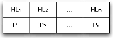
Figure 1. Illustration of the solution representation. HL denotes the half-laps before riders transition, and P indicates the power output of the lead rider for per half lap.

For the transition strategy, there are a moving number of variables representing the strategy, equal to the number of transitions required to complete the race. In the event the riders transition every half lap, this would be 31 transitions (as the riders are not allowed to transition during the first or last 0.75 laps of the race). In the event the riders transition less often, the extraneous variables are simply ignored.

For the pacing strategy, the amount of power levels is fixed to the number of effective half laps. Effective half laps are laps that the riders can transition, and hence the first and last 0.75 laps are represented as single half laps in the genome.

Note that the chosen representation for race strategies is relatively simple. The fitness function takes care of some complicated aspects, such as calculating the effective half lap and considering riders that have dropped out due to exhaustion. This way, we deal with a relatively generic genome that we can then use standard operators on.

It should be noted that we have two-level solutions distributed over a multi-modal solution space, where the transition strategy and pacing strategy are co-constrained. This means that an optimal pacing strategy for a given transition strategy may not be optimal for all transition strategies, and vice versa. Implicitly the minimization of time using the optimal transition strategy requires the optimal pacing strategy to be found; however, due to the complex nature of the dual level problem it may not be possible to find the optimal pacing strategy, and hence sub-optimal solutions for the overall problem may be found.

2.3. Evaluation Function

The aim of the optimization is to minimize time and maximize remaining energy, hence time and energy are used as measures of fitness. In the following, we outline the function as it is used in previous studies [4, 10, 14]. The used physical equations were derived from Martin et al. [2] and adapted to suit team pursuit track cycling conditions.

First, the fitness function needs to assure that the solution is feasible. In case one of the team members runs out of energy they are assumed to have dropped out of the race, however, if two riders run out of energy the solution becomes infeasible and a penalty function is applied. In Algorithm 16 we show our “fitness function,” which simulates a race where the leading cyclist's power output determines the team's speed and thus the energy consumption of the individual team members.

In order to model the time taken and the energy expended by the riders a mathematical model derived from Martin et al. [2] was adapted. To obtain the time taken and energy expended by the lead rider to ride a half lap, a forward integration technique was used, breaking down the time into small Δt of 0.1 s. To calculate the acceleration for riding this Δt we use Equation (1):

$\begin{array}{cc}\Delta \text{KE}=\left(P\times E-C_{D}A\times \left(\frac{1}{2}\rho {\text{v}}^3\right)-\mu \times \left(\text{v}{F}_N\right)\right)\times \Delta t& \left(1\right)\end{array}$

where KE is kinetic energy, P is power, E is mechanical efficiency, C_DA is the frontal area of the bike and rider, v is speed, ρ is air density, μ is a global coefficient of friction, F_N is the weight of the bike and the rider, and t is time. Potential energy was removed from the original equation, as the vertical elevation can be neglected. Note that there is no separate consideration of the air's wind speed, as the event is being held indoors in still air conditions.

The energy needed for the following riders to keep up with the acceleration from the original rider for a time Δt can be calculated using Equation (2):

$\begin{array}{cc}P=\left(C_{D}A\times C_{Draft}\times \frac{1}{2}\rho {\text{v}}^3+\mu \times \left(\text{v}{F}_N\right)+\frac{\Delta \text{KE}}{\Delta t}\right)/E& \left(2\right)\end{array}$

where E is the efficiency of the drive system, ΔKE is calculated using the final velocity of the first rider after acceleration. C_Draft is drafting coefficient of the rider and represents the reduction in the C_DA of a cyclist due to the aerodynamic benefits of drafting in second, third or fourth position. A drafting benefit (C_DRAFT) was added to the original equation, in order to account for the slipstreaming of the following riders.

ALGORITHM 1

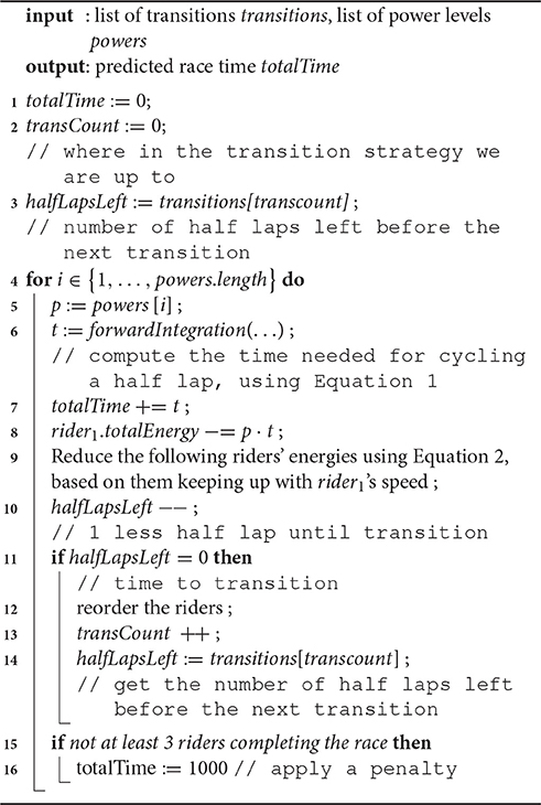
Algorithm 1: Fitness Function

3. Standard Multi-Objective Approach

Our single-level optimization approach is a non-problem specific optimization technique, treating the problem as if it were a standard multi-objective optimization problem. That is, it does not account for the hierarchical nature of the problem, but rather mutates the solution as if it was comprised of only one level. This approach does not change the encoding as we have used a generalized representation for the genome so that standard variation operators can still be used.

In particular, we use two slightly different multi-objective formulations of the optimization problem. In the first formulation, the two-objective problem is the result of considering the race time as one objective and the sum of the cyclists' remaining energy as the second objective. In the second formulation, the first objective is again the race time minimization, however, objectives two to five are the energies remaining of the four cyclists. With this second formulation, we implicitly put an increased focus on creating energy efficient strategies. Also, it allows us to investigate the impacts that different strategies have on the individual racers. A team coach might then realize that the order of the cyclists has to change, or that particular team members need to improve their endurance.

As the first level of the problem (the transition strategy) is discrete in nature, and the second level of the problem (the pacing strategy) is continuous in nature, a range of different mutation methods have to be employed for the two levels. The mutators chosen are standard mutation methods for discrete and continuous variables, as used by Jordan and Kroeger [10].

The discrete variable mutators used on the transition strategy are as follows:

• Random mutation (R): this mutator replaces the value of a chosen gene with a random integer. A gene is chosen with probability 1/m, where m is the effective length of the strategy (as explained in Section 2).

• Creep mutation (C): this mutator is a stepwise mutation that only allows small changes at a time, with the chosen gene “creeping” either up or down by 1. As with random mutation, a gene is chosen with probability 1/m.

The continuous variable mutators used on the pacing strategy are as follows:

• Uniform mutation (U): this mutator replaces the value of a chosen gene with a random value selected between the upper and lower bounds of the acceptable power. A gene is selected with probability 1/n, where n is the length of the pacing strategy.

• Non-uniform mutation (NU): this mutator decreases the probability of mutation as the number of generations increase. This keeps the population from stagnating in the early stages of evolution, but allows for fine-tuning in later stages. This mutator works in the same way as uniform mutation, however rather than replacing the chosen gene, a Gaussian distributed random value that narrows as the number of generations increases is added or subtracted from the gene.

Due to the interrelation between the two levels of our problem, the successful application of a crossover operator is challenging. It would only be reasonable to crossover the lower level part of the problem (the pacing strategy) when the upper level of both parents is the same. As there is no way to ensure this, it was chosen not to use a crossover strategy. An alternative could be to use an informed crossover that knows of the peculiarities of the race, and which merges information and attempts to achieve high quality solutions via repairs. In extensive preliminary experiments, however, we have not been able to design such an operator that was beneficial more often than not.

For our first study, our portfolio of multi-objective optimization algorithms consists of the two algorithms NSGA-II [15] and SPEA2 [16], which are well-established optimization algorithms for multi-objective problems.

3.1. Experimental Design

In order to compare the different combinations of operators and algorithms, we use two population of sizes μ ∈ {10, 100}, and then we explore all combinations. As the computation budget, we use two million function evaluations, as these take approximately 3 h on a Intel Core 2 Duo with 2.4 GHz core speed. Time budgets longer than this could be considered as being impractical for the use on the field prior to an actual race. Due to the stochastic nature of the algorithms, we perform 30 repetitions of each experiment.

In order to create a realistic model of the race, we use realistic parameters as given in Table 1. To model fatigue, we limit the number of laps the lead rider can head a team, and we impose a bound on the amount of energy a rider can expend per half lap. Also, if two or more riders are not able to complete the race due to exhaustion, the strategy is marked infeasible by setting its race time to 1000 s.

TABLE 1

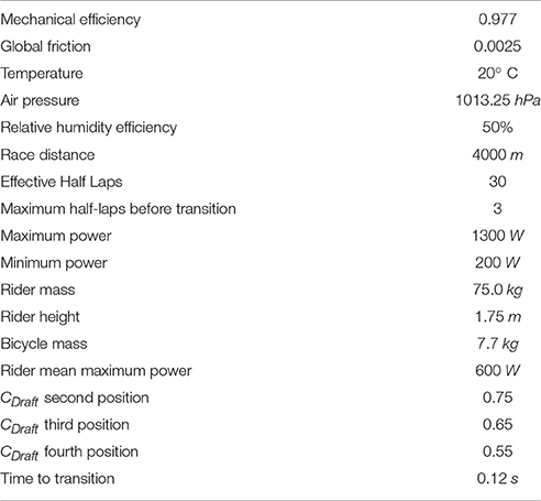
Table 1. Problem parameters.

To compare the performance of the different configurations, we use two approaches. First, we take from the final solution sets the fastest strategies, and then we calculate different statistics based on these best strategies that are found in the 30 independent optimization runs. Second, we calculate the hypervolume that is covered with respect to a chosen reference point. Based on preliminary experiments in which we observed the typical ranges for good feasible solutions, we chose (300s, 220,000kJ) as the reference point for the two-objective case, and (300s, 50,000kJ, 50,000kJ, 50,000kJ, 50,000kJ) for the five-objective case.

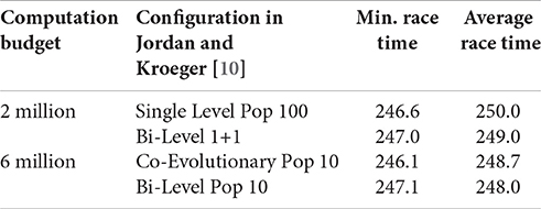
Before we analyse the results, let us briefly recall the best results reported by Jordan and Kroeger [10], who investigated different bi-level and cooperative coevolutionary approaches. From their 10 configurations, we select as benchmarks the ones that resulted in the best minimal and average race times. The following race times will therefore act as our benchmark values:

We implemented everything in the optimization framework jMetal [17]. We have made the fitness function, the code, and the results publicly available: http://cs.adelaide.edu.au/~optlog/research/combinatorial.php.

3.2. Results

In Table 2 we list the results of our first study, where we compare the four variation operators, when used by two multi-objective optimization algorithms. We focus our attention on the race times achieved by the fastest strategy, as these are the likeliest to be implemented by a team coach.

TABLE 2

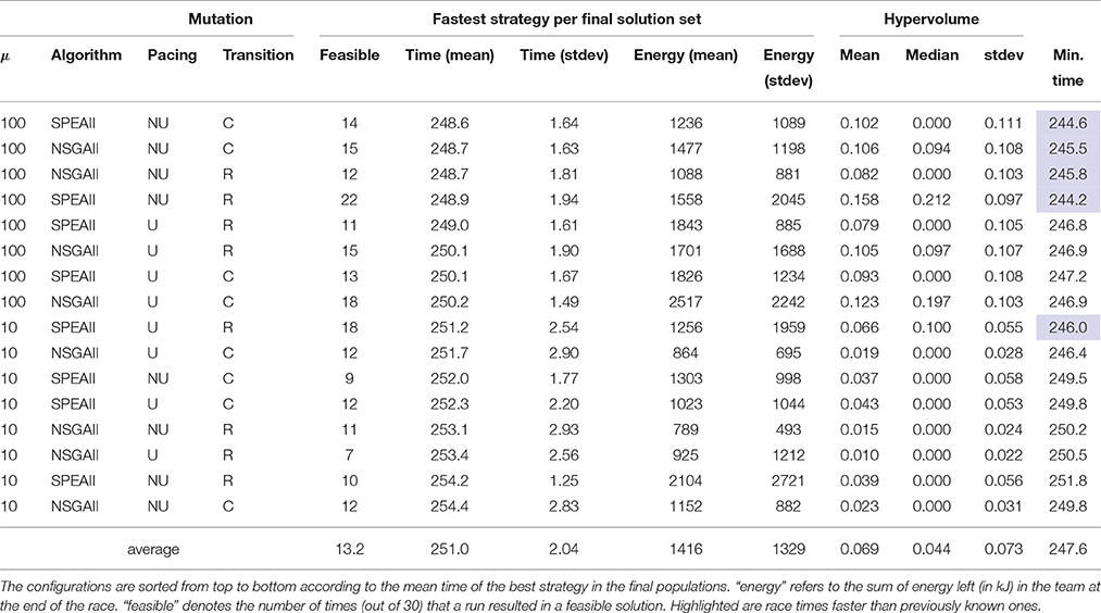
Table 2. Results of the single-level multi-objective study.

First, it is striking that less than 50% of the runs actually return at least one valid strategy. In all other runs, the final solution set contain only infeasible racing strategies that cause the unacceptable dropout of two or more cyclists during the race. At first sight, this renders this approach useless for practical purposes.

However, when our configurations produce feasible solutions, then the best ones significantly outperform those found by Jordan and Kroeger [10]. In particular, our best strategy results in a race time of 244.2 s using two million evaluations, whereas previously 246.1 s was the best result using three times as many evaluations.

Given all 16 tested configurations, general observations are difficult to make. As many runs did not produce feasible solutions, the hypervolume indicator values are difficult to interpret. What we can see is that a larger population (μ = 100) always performed better than a smaller one (μ = 10). When it comes to the used multi-objective algorithm and to the variation operators, no particular combination stands out. It is only that for larger populations the use of the non-uniform pacing mutation (NU) always outperformed the use of the uniform pacing mutation (U).

4. Nested Approach

4.1. Experimental Design

In an attempt to improve the reliability of our previous approaches and inspired by existing approaches, we will next investigate the use of bi-level optimization—with a twist.

First, we extend our portfolio of multi-objective optimization algorithms, which now consists of the algorithms NSGA-II, SPEA2, MO-CMA-ES [18], GREEDY, and GREEDY+RANDOM. We add MO-CMA-ES due its self-adaptive capability and its successful application to continuous problems. As the selection strategies of these multi-objective algorithms focus on the exploration of the entire range (from fast to slow) of race times, we introduce GREEDY and GREEDY+RANDOM as simple selection strategies that are biased toward fast race times. Given a set of λ solutions, GREEDY selects the μ solutions with the fastest race time. As this approach may cause a rapid loss in the transitions strategies' diversity, we also consider GREEDY+RANDOM as a minor modification: the latter selects only the fastest $\frac{\mu }{2}$ solutions, and picks the remaining $\frac{\mu }{2}$ uniformly at random from the λ candidates.

ALGORITHM 2

Algorithm 2: Framework of the Nested Multi-Objective Race Time optimization

Algorithm 2 outlines our framework for the race time optimization. The outer algorithm maintains a set of μ_out solutions, mutating only the transition strategy part. First, μ_out offspring were generated, using the outer algorithm's standard selection strategy (e.g., via binary tournaments). Then, for each such solution the inner algorithm is run in order to optimize the pacing strategy. Each inner algorithm then returns its final population of at most μ_in solutions¹.

The inner algorithms are started with the entire remaining budget of available evaluations. In order to better use the given budget of evaluations, we primarily use convergence as the stopping criterion (for the inner algorithms): if no improvement of the fastest race time is found over a specified number of generations (we chose this number to be 100), the optimization process is ended and the last population is returned. Then, the global budget of evaluations is updated according to the number of evaluations used by the inner algorithms. We proceed until the budget of evaluations is used up.

Note that our approach is loosely related to the hierarchical one used by Wagner et al. and Wagner et al. [4, 14]. There, the problem was split into the outer problem of finding good transition strategies and into the inner problem of finding good pacing strategies for given transition strategies. We are now extending this by using problem-specific variation operators and multi-objective algorithms for the inner and outer problem.

In total, we are considering 4 * 2 * 2 * 3 * 4 = 192 configurations:

• four variation operator combinations: NU-C, NU-R, U-C, U-R (see Section 3)

• one population size of the outer algorithm (μ = 10) and two of the inner algorithm (μ = 10 and μ = 100)

• a two-dimensional and a five-dimensional formulation of the race time minimization problem

• three inner algorithms (NSGAII, SPEA2, MO-CMA-ES) and four outer algorithms (NSGAII, SPEA2, GREEDY, GREEDY+RANDOM)

Just as before, our computation budget per run is two million evaluations, and we perform 30 independent runs of each configuration.

4.2. Results

First, let us have a brief look at the qualitative differences between different configurations. Exemplarily, we list in Table 3 the outcomes of two single optimization runs. Case 1 is the output of a run that used NSGA-II as the inner and outer algorithm, while Case 2 used MO-CMA-ES as the inner algorithm and GREEDY as the outer algorithm. The differences are significant. In the first case, the final strategies are very diverse in race time and remaining energy. For a team coach, this spread in race times by over 2 min (for a 4-min race) might be very confusing. In contrast to this, the solutions in the second case are grouped significantly closer together with times varying less than 3s. Based on the energy left in the team, it appears that MO-CMA-ES succeeded in creating pacing strategies that completely exhaust the cyclists. This was not as apparent in the first case.

TABLE 3

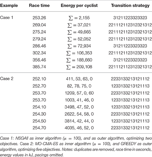
Table 3. Exemplary outputs of the nested optimization.

Next, we can report that all multi-objective bi-level approaches reliably produce feasible race strategies: 5744 of the 5760 experiments resulted in at least one feasible race strategy. No particular configuration has stood out as particularly unreliable. The observed 99.72% reliability to get feasible race strategies is an important improvement over the previously achieved < 50%. At least from a practicality point of view, the nestedness results in algorithms that can be used in the field.

When it comes to the four variation operator combinations, all four appear to perform comparably across the remaining 48 combinations. When NU is used, then the best race strategies are slightly better on average, however, this comes at the cost of an increased variation in the results:

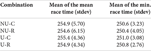
In this first observation, the averaging effect blurs important details. In Figure 2 we therefore show the configurations sorted according to performance. Interestingly, there are always combinations that result in strategies that are not competitive in a real-world situation (see Figure 2A). The average performance is dominated by the configurations that involve the combination NU-R, with NU-C being a relatively close second. Despite this order, we can see in Figure 2B that the other variation operator combinations can be competitive as well.

FIGURE 2

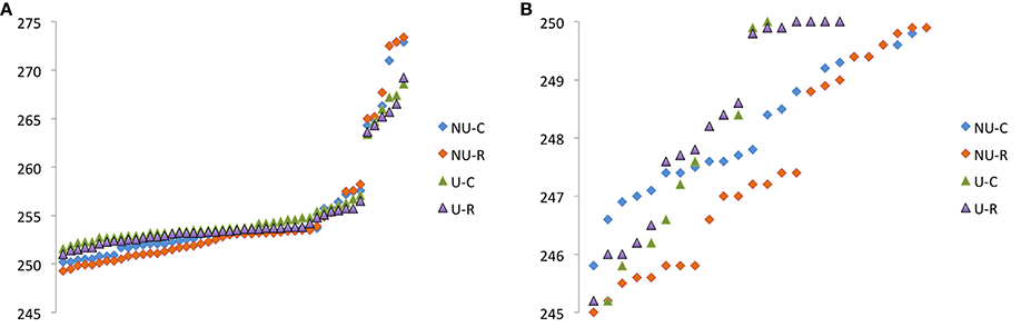
Figure 2. Results of 48 configurations when the variation operator combinations NU-C, NU-R, U-C, and U-R are used. (A) Sorted according to the mean race time (in s) of fastest strategy. Shown are all 192 means. (B) Sorted according to the minimal race time (in s) of fastest strategy. Excerpt shows race times ≤ 250 s.

But which configurations are the best performing ones? Following the previous investigations, we list in Table 4 the configurations that resulted in minimal race times of ≤ 246.1s, which was the benchmark to beat. In summary, we can see that NU-R as a variation operator combination perform the best. For the outer algorithm, an increased pressure toward the race time minimization appears to be useful.

TABLE 4

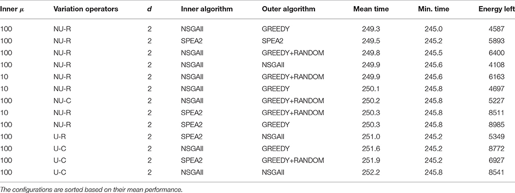
Table 4. Best configurations with race times ≤ 246.1s, which was the best result to beat from Jordan and Kroeger [10].

MO-CMA-ES does not appear in Table 4. In general, its configurations performed just at an average level, neither very good nor very bad. This is interesting, as we have previously seen in Table 3 how effective it is at using up the energy of the team. We conjecture that this capability has been a disadvantage, as it pushed the pacing strategy part of the race strategy too much near local optima from which the outer algorithms had trouble escaping.

Also, it is interesting to note that the five-objective formulations performed not as well as the two-objective ones. This might be due to the inadequacy of the algorithms for higher dimensional spaces, and many-objective optimization algorithms might be more suitable here (see 19, 20, for recent surveys). Another problem is that multi-objective algorithms explore by nature the entire objective space, in an attempt to achieve a good approximation of the true set of trade-offs. This, however, is in contrast to the small part of the objective space that is actually of interest to the team coach. An alternative approach here would be to incorporate the preference more explicitly. In general, techniques to do this have been investigated for over decade [21], they have also recently been brought into the context of many-objective optimization [22].

Coming back to our single level approach, we have to remark that we might not be using the full potential of this approach as the constraints are handled inefficiently by our penalty. We noticed that a direct consideration of the energy levels of the riders inside a variation operator is difficult, as the race is simulated. An improvement here might be the use of a repair operator. The design of such an operator is not straightforward, as the problem cannot be decomposed and this operator would have to quickly consider roughly 17 decision variables without letting the solution quality deteriorate too much.

To conclude, we have seen that the nesting of algorithms yielded feasible solutions reliably. The previously best known solution for this problem resulted in a race time of 246.11 s. We improved upon this with race times of 244.24 s (Section 3.1). Needless to say, such a gap in solution quality can make the difference between no medal and a gold medal.

For the record, the following is our best solution found, which is an improvement by 1.87 s over the previous best:

  final race time: 244.24
  remaining energy: 245
  strategy: 313121212121131123
  powers: 1194 550 741 200 794 977 928 200
  561 455 237 1229 808 208 200 631 200 1177

5. Summary

In this article, we addressed the problem of designing fast team strategies for track cycling. In addition to the traditional minimization of the race times, we considered the amount of energy that the riders have left at the end of the race. For the team coach this extension has the benefit that a diverse set of strategies can be investigated through the multi-objective space. Also, the coach will see the trade-offs between fast strategies and slightly slower ones, where the latter allow the team to conserve energy for future races and to recover faster.

To solve this multi-objective problem, we applied different state-of-the-art algorithms with problem-specific variation operators in two different ways. In the first approach, we used them in their standard way. We quickly noticed that computation time was wasted by investigating “slow” parts of the objective space. Also, feasible solutions were created in less than 50% of the time. To deal with these problems, we nested a biased algorithm multi-objective algorithm (with the convergence criterion based on race time minimization) inside the standard one in the second approach.

Although the inner algorithms explored portions of the search space that are not of interest to the team coach (i.e., slow strategies are found), the increased diversity and bias paid off, and faster race times were found with our nested multi-objective approach than with the regular multi-objective approach. In particular we improve the previous best known race strategy by 1.87 s.

Future work on this problem will go into three different directions. First, we will investigate more systematically the conditions under which nesting multi-objective algorithms can be beneficial in general, which might include theoretical investigations. The insights gained there might lead toward general recommendations for hierarchical programming. Second, we will validate and fine-tune the model using real races to increase the accuracy of the predictions. Third, we will explore the conversion of the research into a decision support tool for team coaches. This includes increased computational speed, fine-tuning of the algorithms, and the support for interactive optimization.

The fitness function, the code, and the results have been made publicly available: http://cs.adelaide.edu.au/~optlog/research/combinatorial.php.

Author Contributions

MW has been responsible for coding, running the experiments, analysing the results, and writing the article.

Funding

This work has been partially funded by the ARC Discovery Early Career Researcher Award DE160100850.

Conflict of Interest Statement

The author declares that the research was conducted in the absence of any commercial or financial relationships that could be construed as a potential conflict of interest.

Acknowledgments

The author would like to thank Dr. Tammie Ebert from Cycling Australia and Dr. David Martin from the Australian Institute of Sport Cycling Program for their valuable support. Also, the author would like to thank Claire Diora Jordan for her valuable contributions to this project. Dedicated to the late Dr. Trent Kroeger.

Footnotes

1. ^Note that some inner algorithms may return less than μ_in solutions, as some return only non-dominated solutions.

References

1. de Koning JJ, Bobbert MF, Foster C. Determination of optimal pacing strategy in track cycling with an energy flow model. J Sci Med Sport. (1999) 2:266–77. doi: 10.1016/S1440-2440(99)80178-9

PubMed Abstract | CrossRef Full Text | Google Scholar

2. Martin JC, Gardner AS, Barras M, Martin DT. Modeling sprint cycling using field-derived parameters and forward integration. Med Sci Sports Exerc. (2006) 38:592–7. doi: 10.1249/01.mss.0000193560.34022.04

PubMed Abstract | CrossRef Full Text | Google Scholar

3. Olds TS, Norton KI, Lowe EL, Olive S, Reay F, Ly S. Modeling road-cycling performance. J Appl Physiol. (1995) 78:1596.

PubMed Abstract | Google Scholar

4. Wagner M, Day J, Jordan D, Kroeger T, Neumann F. Evolving pacing strategies for team pursuit track cycling. In: 9th Metaheuristics International Conference (MIC 2011). Udine: Universita degli Studi di Udine (2011). p. 491–500.

5. Migdalas A, Pardalos PM. Editorial: hierarchical and bilevel programming. J Glob Optim. (1996) 8:209–15. doi: 10.1007/BF00121265

CrossRef Full Text | Google Scholar

6. Bard JF. Practical Bilevel Optimization: Algorithms and Applications. New York, NY: Springer (1998).

Google Scholar

7. Deb K, Sinha A. An efficient and accurate solution methodology for bilevel multi-objective programming problems using a hybrid evolutionary-local-search algorithm. Evol Comput. (2010) 18:403–49. doi: 10.1162/EVCO_a_00015

PubMed Abstract | CrossRef Full Text | Google Scholar

8. Anandalingam G, Friesz TL. Hierarchical optimization: an introduction. Ann Operat Res. (1992) 34:1–11. doi: 10.1007/BF02098169

CrossRef Full Text | Google Scholar

9. Colson B, Marcotte P, Savard G. An overview of bilevel optimization. Ann Operat Res. (2007) 153:235–56. doi: 10.1007/s10479-007-0176-2

CrossRef Full Text | Google Scholar

10. Jordan CD, Kroeger T. An evolutionary algorithm for bilevel optimisation of Men's Team Pursuit Track Cycling. In: 2012 IEEE Congress on Evolutionary Computation. Brisbane, QLD (2012). p. 1–8.

11. Herskovits J, Leontiev A, Dias G, Santos G. Contact shape optimization: a bilevel programming approach. Struct Multidiscip Optim. (2000) 20:214–21. doi: 10.1007/s001580050149

CrossRef Full Text | Google Scholar

12. Eichfelder G. Multiobjective bilevel optimization. Math Prog. (2010) 123:419–49. doi: 10.1007/s10107-008-0259-0

CrossRef Full Text | Google Scholar

13. Talbi EG. Metaheuristics: From Design to Implementation. Hoboken, NJ: Wiley (2009).

Google Scholar

14. Wagner M, Day J, Jordan D, Kroeger T, Neumann F. Evolving pacing strategies for team pursuit track cycling. In: Di Gaspero L, Schaerf A, Stützle T, editors. Advances in Metaheuristics. New York, NY: Springer (2013). p. 61–76.

Google Scholar

15. Deb K, Pratap A, Agrawal S, Meyarivan T. A fast and elitist multiobjective genetic algorithm: NSGA-II. IEEE Trans Evol Comput. (2002) 6:182–97. doi: 10.1109/4235.996017

CrossRef Full Text | Google Scholar

16. Zitzler E, Laumanns M, Thiele L. SPEA2: improving the strength pareto evolutionary algorithm for multiobjective optimization. In: Giannakoglou KC, Tsahalis DT, Périaux J, Papailiou KD, Fogarty T, editors. Evolutionary Methods for Design Optimization and Control with Applications to Industrial Problems. Athens, International Center for Numerical Methods in Engineering (Cmine) (2001). p. 95–100.

17. Durillo JJ, Nebro AJ, Alba E. The jMetal framework for multi-objective optimization: design and architecture. In: IEEE Congress on Evolutionary Computation (CEC 2010). Berlin; Heidelberg: IEEE Press (2010). p. 4138–325.

18. Igel C, Hansen N, Roth S. Covariance matrix adaptation for multi-objective optimization. Evol Comput. (2007) 15:1–28. doi: 10.1162/evco.2007.15.1.1

PubMed Abstract | CrossRef Full Text | Google Scholar

19. Chand S, Wagner M. Evolutionary many-objective optimization: a quick-start guide. Surv Oper Res Manage Sci. (2015) 20:35–42. doi: 10.1016/j.sorms.2015.08.001

CrossRef Full Text | Google Scholar

20. Li B, Li J, Tang K, Yao X. Many-objective evolutionary algorithms: a survey. ACM Comput Surv. (2015) 48:13:1–13:35. doi: 10.1145/2792984

CrossRef Full Text | Google Scholar

21. Rachmawati L, Srinivasan D. Preference incorporation in multi-objective evolutionary algorithms: a survey. In: IEEE International Conference on Evolutionary Computation. Vancouver, BC (2006). p. 962–8.

22. Mohammadi A, Omidvar MN, Li X, Deb K. Integrating user preferences and decomposition methods for many-objective optimization. In: IEEE Congress on Evolutionary Computation, CEC. IEEE. Beijing (2014). p. 421–8.

Google Scholar