Study on Parameter Choice Methods for the RFMP with Respect to Downward Continuation

1. Introduction

The gravitational field of the Earth is an important reference in the geosciences. It is an indicator for mass transports and mass reallocation on the Earth's surface. These displacements of masses can be caused by ocean currents, evaporation, changes of the groundwater level, ablating of continental ice sheets, changes in the mean sea level or climate change (see e.g., [1, 2]).

However, it is difficult to model the gravitational field, because terrestrial measurements are not globally available. In addition, the points of measurement on the sea are more scattered than those on the continents. This has motivated the launch of satellite missions with a focus on the gravitational field (see e.g., [3–6]). Naturally, those data are given at a satellite orbit, not on the Earth's surface. Additionally, the measurements are only given pointwise and are afflicted with noise. The problem of getting the potential from the satellite orbit onto the Earth's surface is the so-called downward continuation problem, which is a severely unstable and, therefore, ill-posed inverse problem (see e.g., [7, 8]).

Traditionally, the gravitational potential of the Earth has been represented in terms of orthogonal spherical polynomials (i.e., spherical harmonics Y_{n, j}, see e.g., [9–11]) as in the case of the Earth Gravitational Model 2008 (EGM2008, see [12]). An advantage of this representation is that the upward continuation operator Ψ which maps a potential F from the Earth's surface (which we assume here to be the unit sphere Ω) to the orbit rΩ with r > 1 has the singular value decomposition

$\begin{array}{ll}(\text{Ψ}F)(x)={\displaystyle \sum _{n=0}^{\infty }}{\displaystyle \sum _{j=-n}^n}{\langle F,Y_{n,j}\rangle }_{L^2(\Omega )}{r}^{-n}{Y}_{n,j}^r(x),& (1)\end{array}$

where $Y_{n,j}^r(x):=\frac{1}{r}{Y}_{n,j}(\frac{x}{r})$, x ∈ rΩ. Its inverse is, therefore, given by

$\begin{array}{l}{\text{Ψ}}^{+}G={\displaystyle \sum _{n=0}^{\infty }}{\displaystyle \sum _{j=-n}^n}{\langle G,Y_{n,j}^r\rangle }_{L^2(r\Omega )}{r}^n{Y}_{n,j}\\ ={\displaystyle \sum _{n=0}^{\infty }}{\displaystyle \sum _{j=-n}^n}{\langle G,Y_{n,j}^r\rangle }_{L^2(r\Omega )}{\sigma }_n^{-1}{Y}_{n,j}& (2)\end{array}$

in the sense of L²(Ω) and for all G ∈ Ψ(L²(Ω)) ⊂ L²(rΩ). Note that the singular values of Ψ⁺, which are given by ${({\sigma }_n^{-1})}_n={(r^n)}_n$, increase exponentially. For details, see [8, 13].

Numerous methods have been developed for solving such linear ill-posed inverse problems. Recently, the RFMP and the ROFMP were constructed as more flexible algorithms which can iteratively construct a kind of a “best basis” for such problems. This yields additional features like a multi-scale analysis and a locally adapted resolution. The methods are based on techniques which were constructed for approximation problems mainly on the Euclidean space (see [14–16]). One of the enhancements of the RFMP and the ROFMP is the introduction of a Tikhonov-Phillips regularization for handling ill-posed problems.

So far, the choice of the regularization parameter of the RFMP and the ROFMP, which weights the regularization term relative to the data misfit, has not been addressed sufficiently, which is why we report here about our corresponding numerical experiments for the regularization of the downward continuation problem with the RFMP and the ROFMP. For this purpose, numerous parameter choice strategies were compared regarding their performance for some selected scenarios.

A parameter choice strategy is a method that determines a value for the regularization parameter. Its input leads to a classification (see e.g., [17]):

• a-priori methods use information on the noise level and the noise-free solution which is usually not known in practice. Therefore, we do not consider such methods.

• a-posteriori methods require the noisy data and the noise level or at least an estimate of it.

• data-driven methods (sometimes also called “heuristic methods”) only work with the noisy data.

Many methods yield a parameter λ such that a function f(λ) falls below a prescribed threshold or such that λ minimizes a function f. Sometimes a tuning parameter (such as the aforementioned threshold) is required. Note that, for stochastic noise, data-driven methods yield converging regularization methods with good performance in practice (cf. [18, 19]).

The outline of this paper is as follows. Section 2 gives a short introduction to the RFMP and its enhancement, the ROFMP. For both algorithms, the essential theoretical results are recapitulated. In Section 3, the parameter choice methods under consideration for the RFMP and ROFMP are summarized and details of their implementation for the test cases are explained. In Section 4, the relevant details of the considered test scenarios are outlined. Section 5 analyzes and compares the results for the various parameter choice strategies.

2. RFMP

In this section, we briefly recapitulate the RFMP, which was introduced in [20–23], and an orthogonalized modification of it (see [13, 24]). It is an algorithm for the regularization of linear inverse problems.

According to [13, 23, 25], we use an arbitrary Hilbert space ${H}\subset L^2(\Omega )$. This space can be L²(Ω) itself, but it can, for instance, also be a Sobolev subspace of L²(Ω). It is chosen for the regularization term (see below) based on numerical experiences or prior knowledge about the solution if available.

Let an operator ${F}:{H}\to {ℝ}^l$ be given which is continuous and linear. Concerning the downward continuation, we have a vector y ∈ ℝ^l of measurements at a satellite orbit, that means our data are given pointwise. The inverse problem consists of the determination of a function $F\in {H}$ such that

$\begin{array}{ll}{F}F=\mathbf{y}={((\text{Ψ}F)(x_j))}_{j=1,\dots ,l},& (3)\end{array}$

where (x_j)_j=1,…,l is a set of points at satellite height. In the following, we use bold letters for vectors in ℝ^l.

To find an approximation for our function F, we need to have a set of trial functions ${D}\subset {H}\backslash \left\{0\right\}$, which we call the dictionary. Our unknown function F is expanded in terms of dictionary elements, that means we can represent it as $F=\sum _{k=1}^{\infty }{\alpha }_k{d}_k$ with ${\alpha }_k\in ℝ$ and $d_k\in {D}$ for all $k\in \mathbb{N}$.

2.1. The Algorithm

The idea of the RFMP is the iterative construction of a sequence of approximations (_Fn)n. This means that we add a basis function d_k from the dictionary to the approximation in each step. This basis function is furthermore equipped with a coefficient α_k.

Since the considered inverse problem is ill-posed, we use the Tikhonov-Phillips regularization, that is, our task is to find a function F which minimizes

$\begin{array}{ll}\Vert \mathbf{y}-{F}F{\Vert }_{{ℝ}^l}^2+\lambda \Vert F{\Vert }_{{H}}^2.& (4)\end{array}$

That means, if we have the approximation F_n up to step n, our greedy algorithm chooses α_n+1 ∈ ℝ and $d_{n+1}\in {D}$ such that

$\begin{array}{ll}\Vert \mathbf{y}-{F}(F_n+{\alpha }_{n+1}{d}_{n+1}){\Vert }_{{ℝ}^l}^2+\lambda \Vert F_n+{\alpha }_{n+1}{d}_{n+1}{\Vert }_{{H}}^2& (5)\end{array}$

is minimized. Here, λ > 0 is the regularization parameter.

We can state the following algorithm for the RFMP.

ALGORITHM 2.1

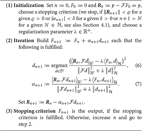
Algorithm 2.1 Let y ∈ ℝ^l and an operator ${F}:{H}\to {ℝ}^l$ (linear and continuous) be given.

The maximization, which is necessary to get d_n+1, is implemented by evaluating the fraction for all $d\in {D}$ in each iteration and picking a maximizer. Since many involved terms can be calculated in a preprocessing, the numerical expenses can be kept low (see [22]). For a convergence proof of the RFMP, we refer to [25]. Briefly, under certain conditions, one can show that the sequence (_Fn)n converges to the solution F_∞ of the Tikhonov-regularized normal equation

$\begin{array}{ll}({{F}}^{*}{F}+\lambda {I})F_{\infty }={{F}}^{*}y,& (8)\end{array}$

where ${I}$ is the identity operator and ${{F}}^{*}$ is the adjoint operator to ${F}$.

2.2. ROFMP

The ROFMP is an advancement of the RFMP from the previous section.

The basic idea is to project the residual onto the span of the chosen vectors, i.e.,

$\begin{array}{ll}{{V}}_n:=span\left\{{F}{d}_1,\dots ,{F}{d}_n\right\}\subset {ℝ}^l,& (9)\end{array}$

and then adjust the previously chosen coefficients in such a way that the residual is afterwards contained in the orthogonal complement of the span. Since this so-called backfitting (cf. [14, 15]) might not be optimal, we implement the so-called prefitting (cf. [16]), where the next function and all coefficients are chosen simultaneously to guarantee optimality at every single stage of the algorithm. Moreover, let ${{W}}_n:={{V}}_n^{\perp }$ and let the orthogonal projections on ${{V}}_n$ and ${{W}}_n$ be denoted by ${{P}}_{{{V}}_n}$ and ${{P}}_{{{W}}_n}$, respectively. All in all, our aim is to find

$\begin{array}{l}({\alpha }_{n+1},d_{n+1})=\\ {\displaystyle \underset{\alpha \in ℝ,d\in {D}}{argmin}}\left(\Vert {\mathbf{R}}_n-\alpha {{P}}_{{{W}}_n}{F}d{\Vert }_{{ℝ}^l}^2+\lambda \Vert F_n-\alpha B_n(d)+\alpha d{\Vert }_{{H}}^2\right).& (10)\end{array}$

Here,

$\begin{array}{ll}{\displaystyle \sum _{i=1}^n}{\beta }_i^{(n)}(d){F}{d}_i={{P}}_{{{V}}_n}({F}d)& (11)\end{array}$

and, thereby, we set

$\begin{array}{ll}{B}_n(d):={\displaystyle \sum _{i=1}^n}{\beta }_i^{(n)}(d)d_i\in {H}.& (12)\end{array}$

The updated coefficients for the expansion at step n + 1 are given by

$\begin{array}{lll}{\alpha }_i^{(n+1)}& :={\alpha }_i^{(n)}-{\alpha }_{n+1}{\beta }_i^{(n)}(d_{n+1}),i=1,\dots ,n,& (13)\end{array}$

$\begin{array}{lll}{\alpha }_{n+1}^{(n+1)}& :={\alpha }_{n+1}.& (14)\end{array}$

The ROFMP is summarized in Algorithm 2.2. For practical details of the implementation, see [13].

ALGORITHM 2.2

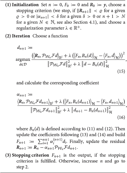
Algorithm 2.2 Let a dictionary ${D}\subset {H}\backslash \left\{0\right\}$, a data vector y ∈ ℝ^l and an operator ${F}:{H}\to {ℝ}^l$ (linear and continuous) be given.

Remark 2.1. If we choose $d_i\in {D}$ and α_i as in Algorithm 2.2 and update the coefficients as in Equations (13) and (14), we obtain for the regularized case (λ > 0) that R_n is, in general, not orthogonal to ${{V}}_n$ for all n ∈ ℕ₀, that means

$\begin{array}{ll}{\mathbf{R}}_n\notin {{W}}_n.& (17)\end{array}$

In [13], it was shown that, with the assumptions from Remark 2.1, there exists a number N: = N(λ) such that

$\begin{array}{ll}{\mathbf{R}}_n={\mathbf{R}}_N\text{ for all }n\ge N.& (18)\end{array}$

That means we get a stagnation of the residual. This is a problem since the ROFMP is not able to reconstruct a certain contribution of the signal which lies in ${{V}}_n$. Therefore, we modify the algorithm based on iterated Tikhonov-Phillips regularization. That means we run the algorithm for a given number of iterations (in our case K > 0), then interrupt the process and start the algorithm with the latest residual R_K. This action is called restart (or repetition) and it is recurringly executed after every K iterations. In order not to lose information we want to maintain the entire expansion F_n during the process. For this purpose, we need an additional notation: we add a further subscript j to the expansion F_n. Note that we have two levels of iterations here. The upper level is associated to the restart procedure and is enumerated by the second subscript j. The lower iteration level is the previously described ROFMP iteration with the first subscript n. We denote the current expansion by

$\begin{array}{ll}{F}_{n,j}:=F_{K,j-1}+{\displaystyle \sum _{i=1}^n}{\alpha }_{i,j}^{(n)}{d}_{i,j},& (19)\end{array}$

where F_0,1 := 0 and F_0,j := F_K,j−1. In analogy to the previous definitions, the residual can be defined in the following way:

$\begin{array}{lll}{\mathbf{R}}_{n,j}& :=& \mathbf{y}-{F}{F}_{n,j},1\le n\le K,j\ge 1\text{and}\\ {\mathbf{R}}_{0,j}& :=& \mathbf{y}-{F}{F}_{K,j-1}={\mathbf{R}}_{K,j-1}.& (20)\end{array}$

That means, after K iterations, we keep the previously chosen coefficients fixed and restart the ROFMP with the residual of the step before. All in all, we have to solve

$\begin{array}{l}({\alpha }_{n+1,j},d_{n+1,j})\\ ={\displaystyle \underset{\alpha \in ℝ,d\in {D}}{argmin}}\left(\Vert {\mathbf{R}}_{n,j}-\alpha {{P}}_{{{W}}_{n,j}}{F}d{\Vert }_{{ℝ}^l}^2+\lambda \Vert F_{n+1,j}{\Vert }_{{H}}^2\right)& (21)\end{array}$

and update the coefficients in the following way

$\begin{array}{ll}{\alpha }_{i,j}^{(n+1)}:={\alpha }_{i,j}^{(n)}-{\alpha }_{n+1,j}{\beta }_{i,j}^{(n)}(d_{n+1,j}),i=1,\dots ,n.& (22)\end{array}$

We summarize for the expansion F_K,m, which is the approximation produced by the ROFMP after m restarts:

$\begin{array}{ll}{T}_m:=F_{K,m}={\displaystyle \sum _{j=1}^m}{\displaystyle \sum _{i=1}^K}{\alpha }_{i,j}^{(K)}{d}_{i,j}.& (23)\end{array}$

In analogy to the RFMP, we obtain a similar convergence result for the ROFMP. That is, under certain technical conditions, the sequence (_Tm)m converges in the Hilbert space ${H}$. For further details, we refer to [13, 24].

3. Parameter Choice Methods

The choice of the regularization parameter λ is crucial for the RFMP and the ROFMP, as for every other regularization method. In this section, we briefly summarize the parameter choice methods which we test for the RFMP and the ROFMP. This section is basically conform to [18, 19].

3.1. Introduction

The Earth Gravitational Model 2008 (EGM2008, see [12]) is a spherical harmonics model of the gravitational potential of the Earth up to degree 2190 and order 2159. We use this model up to degree 100 for the solution F in our numerical tests. For checking the parameter choice methods, we generate different test cases that means test scenarios which vary in the satellite height, the noise-to-signal ratio and the data grid. Based on the chosen function F, our dictionary contains all spherical harmonics up to degree 100 that means our approximation F from the algorithm has the following representation

$\begin{array}{ll}F={\displaystyle \sum _{n=0}^{100}}{\displaystyle \sum _{j=-n}^n}{\alpha }_{n,j}{Y}_{n,j},\text{ where not all }{\alpha }_{n,j}\text{ vanish}.& (24)\end{array}$

This is a strong limitation, but higher degrees would essentially enlarge the computational expenses.

Moreover, for the stabilization of the solution, we use the norm of the Sobolev space ${H}:={H}({(a_n)}_n;\Omega )$ which is constructed with

$\begin{array}{ll}{a}_n:={\left(n+\frac{1}{2}\right)}^2,n\in {\mathbb{N}}_0,& (25)\end{array}$

see [26]. This Sobolev space contains all functions F on Ω which fulfill

$\begin{array}{ll}{\displaystyle \sum _{n=0}^{\infty }}{\displaystyle \sum _{j=-n}^n}{a}_n^2{\langle F,Y_{n,j}\rangle }_{L^2(\Omega )}^2<\infty .& (26)\end{array}$

The inner product of functions $F,G\in {H}$ is given by

$\begin{array}{ll}{\langle F,G\rangle }_{{H}}:={\displaystyle \sum _{n=0}^{\infty }}{\displaystyle \sum _{j=-n}^n}{a}_n^2{\langle F,Y_{n,j}\rangle }_{L^2(\Omega )}{\langle G,Y_{n,j}\rangle }_{L^2(\Omega )}.& (27)\end{array}$

The particular sequence ${(a_n)}_n={({(n+\frac{1}{2})}^2)}_n$ was chosen, because preliminary numerical experiments showed that the associated regularization term yielded results with an appropriate smoothness.

In our test scenarios, we use a finite set {_{λk}k=1,…,100} of 100 regularization parameters (for details, see Section 4.4). The approximate solution of the inverse problem as an output of the RFMP/ROFMP corresponding to the regularization parameter λ_k and the data vector y is denoted by x_k. This notation is introduced to avoid confusions with the functions F_n which occur at the n-th step of the iteration within the RFMP.

In practice, we deal with noisy data y^ε where the noise level ε is defined by

$\begin{array}{ll}\epsilon :=\text{N}2\text{S}·\Vert \mathbf{y}\Vert {}_{{ℝ}^l}/\sqrt{l},& (28)\end{array}$

where l is the length of the data vector y and N2S is called the noise-to-signal ratio. The corresponding result of the RFMP/ROFMP for the regularization parameter λ_k and the noisy data vector y^ε is called $x_k^{\epsilon }$. Due to the convergence results for the RFMP/ROFMP (see Equation 8), we introduce the linear regularization operators ${{R}}_k:{ℝ}^l\to {H}$,

$\begin{array}{ll}{{R}}_k:={({{F}}^{*}{F}+{\lambda }_k{I})}^{-1}{{F}}^{*}& (29)\end{array}$

and assume x_k to be ${{R}}_k\mathbf{y}$ and $x_k^{\epsilon }$ to be ${{R}}_k{\mathbf{y}}^{\epsilon }$, though this could certainly only be guaranteed for an infinite number of iterations.

Due to the importance of the regularization parameter, we summarize in the next section some methods for the choice of this parameter λ. For the comparison of the methods, we have to define the optimal regularization parameter λ_kopt. We do this by minimizing the difference between the exact solution x and the regularized solution $x_k^{\epsilon }$ corresponding to the parameter λ_k and noisy data.

$\begin{array}{ll}{k}_{\text{opt}}:={\displaystyle \underset{k\in \left\{1,\dots ,100\right\}}{argmin}}\Vert x-x_k^{\epsilon }\Vert {}_{L^2(\Omega )}.& (30)\end{array}$

Then we evaluate the results by computing the so-called inefficiency by

$\begin{array}{ll}\frac{\Vert x-x_{k_{*}}^{\epsilon }\Vert {}_{L^2(\Omega )}}{\Vert x-x_{k_{opt}}^{\epsilon }\Vert {}_{L^2(\Omega )}},& (31)\end{array}$

where λ_k* is the regularization parameter selected by the considered parameter choice method. For the computation of the inefficiency, we use the L²(Ω)-norm, since our numerical results led to a better distinction of the different inefficiencies than by using the ${H}$-norm. However, the tendency regarding “good” and “bad” parameters were the same in both cases.

In practical cases, the exact solution is usually unknown such that k_opt is a theoretical object only. Parameter choice methods, such as those which are used for the experiments here, provide us with a way to estimate (in some sense) a regularization parameter λ_k* which yields a solution which is expected to be close to the unknown exact solution. The inefficiency quantifies the accuracy of this estimate by comparing $x_{k_{*}}^{\epsilon }$ with the theoretically optimal regularized solution $x_{k_{opt}}^{\epsilon }$. The closer the obtained inefficiency is to 1, the better the parameter choice method performs.

Note that the norms which occur in the several parameter choice methods can be computed with the help of the singular value decomposition. However, we use the singular values of Ψ (see Equations 1 and 3) for this purpose, because the singular value decomposition of ${F}$ is unavailable. This certainly causes an inaccuracy in our calculations, but appears to be unavoidable for the sake of practicability.

3.2. Parameter Choice Methods

Table 1 shows the different parameter choice methods we tested and introduces their abbreviations. The tuning parameters are chosen in accordance to [18, 19]. For the choice of the maximal index $\widehat{K}$, see Section 4.5.

TABLE 1

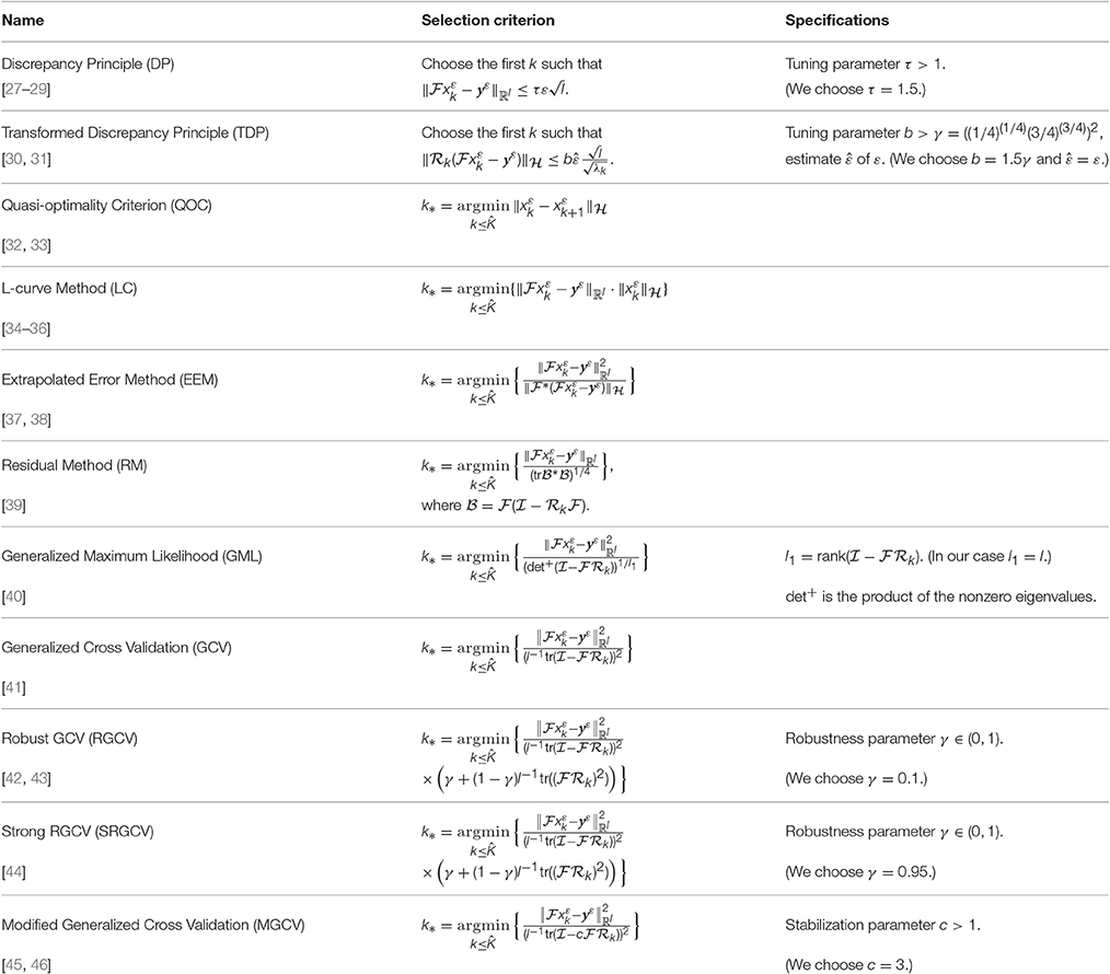
Table 1. The parameter choice methods and their specifications.

The DP of [27–29] tries to balance the norm of the residual and the noise level ε for a good regularization. It requires knowledge of ε which we provide in our tests. The TDP of [30, 31] tries to deal with the instability of the DP if the noise level is not known. It is designed to work with an estimate $\widehat{\epsilon }$ of ε.

The QOC goes back to [32, 33] and its continuous version tries to minimize the norm $\Vert \lambda \frac{d}{d\lambda }{x}_{\lambda }^{\epsilon }\Vert$. By using the difference quotient instead of the derivative for our discrete parameters ${\lambda }_k={\lambda }_0{q}_{\lambda }^k$ (see Section 4.4), we obtain the method as in Table 1.

The LC (cf. [34–36]) is based on the fact that a log-log plot of $(\Vert {F}{x}_k^{\epsilon }-{\mathbf{\text{y}}}^{\epsilon }\Vert ,\Vert x_k^{\epsilon }\Vert )$ often is L-shaped. The points on the vertical part correspond to under-smoothed solutions, where the horizontal part consists of points due to over-smoothed solutions. This suggests that the “corner” defines a good value for the regularization parameter. Note that usually the method is applied manually and its automating can be difficult.

The EEM of [37, 38] chooses the regularization parameter by minimizing an estimate of the error $\Vert x-x_k^{\epsilon }\Vert$ found by an extrapolation procedure. The RM of [39] is based on minimizing a certain weighted form of the norms of the residuals, where the weighting penalizes under-smoothing parameter values.

It is known that the Tikhonov regularized solution for discrete data with independent Gaussian errors can be interpreted as a Bayes estimate of x if x is endowed with the prior of a certain zero mean Gaussian stochastic process (cf. [47]). With this interpretation, the GML estimate was derived by [40] and formulated for stochastic white noise where knowledge of the noise level ε is not needed.

The GCV of [41] uses the following idea: consider all the “leave-one-out” regularized solutions and choose the parameter which minimizes the average of the prediction errors using each solution to predict the data value that was left out. Note that the computation of all these regularized solutions is not necessary for this. A detailed derivation can be found in [47]. Several modifications and extensions of the method such as RGCV (cf. [42, 43]), SRGCV (cf. [44]) and MGCV (cf. [45, 46]) have been developed to deal with instabilities of the GCV. Note that for certain choices of the robustness/stabilization parameter these variants correspond to GCV.

4. Evaluation

4.1. Specifications for the Algorithm

In Sections 2.1 and 2.2, we mentioned that we need to define stopping criteria for our algorithm. We state the following stopping criteria for the RFMP and ROFMP (see also Algorithms 2.1 and 2.2).

• $\Vert R_{n+1}{\Vert }_{{ℝ}^l}<\varrho$ for a given ϱ > 0 (in our case, this is the N2S),

• n+1 > N for a given N ∈ ℕ (in our case, N = 10, 000 because of our computing capacity),

• |α_n+1| < δ for a given δ > 0 (in our case δ = 10⁻⁶).

In the case of the ROFMP, we choose K = 200 for the restart.

4.2. The Data Grids

Figure 1 shows two data grids which we use for our experiments. First of all, the Reuter grid (see [48]) is an example of a regular data grid on the sphere. Second, we have a set of irregularly distributed data points on a grid which we refer to as the scattered grid in the following and which was first used in [13]. The latter grid tries to imitate the distribution of measurements along the tracks of a satellite. It possesses additional shorter tracks and, thus, a higher accumulation of data points at the poles and only fewer tracks in a belt around the equator.

FIGURE 1

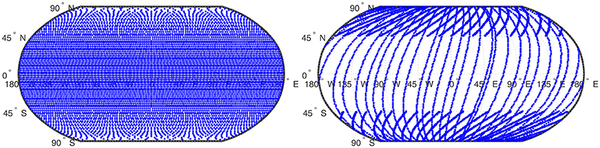
Figure 1. Reuter grid with 8514 points (Left) and scattered grid with 8,500 points (Right).

4.3. Noise Generation

For our various scenarios, we get our noisy data if we add white noise to our data values or we add colored noise that is obtained by an autoregression process. Additionally, we test some local noise.

4.3.1. White Noise Scenario

For white noise, we add Gaussian noise corresponding to a certain noise-to-signal ratio N2S to the particular value of each datum, that means we get our noisy data by

$\begin{array}{ll}{y}_i^{\epsilon }=(1+\text{N}2\text{S}·{ϵ}_i)y_i=\text{N}2\text{S}·y_i{ϵ}_i+y_i,i=1,\dots ,l,& (32)\end{array}$

where y_i are the components of y and ${ϵ}_i~{N}(0,1)$, that means every ϵ_i is a standard normally distributed random variable.

4.3.2. Colored Noise Scenario

Since our scattered grid tries to imitate tracks of satellites, we can assume that we have a chronology of the data points for each track. To obtain some sort of colored noise, we use an autoregression process of order 1 (briefly: AR(1)-process, see [49]) with whom we simulate correlated noise.

A stochastic process {ϵ_i, i ∈ ℤ} is called an autoregressive process of order 1, if ϵ_i = αϵ_i−1+ε_i, |α| <1, where ${\epsilon }_i~{N}(0,1)$. In the case of our simulation, we start with ${ϵ}_1~{N}(0,1)$ and run the recursion for a fixed α ∈ (−1, 1), which we determined at random.

For each track of the scattered grid, we apply this autoregression process (for the tracks, see Figure 2) and obtain $y_i^{\epsilon }$ as in Equation (32) using the ϵ_i from above.

FIGURE 2

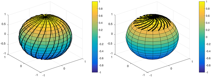
Figure 2. The track sets of the scattered grid (Left, Right). For the South pole, we have an analogous point distribution.

4.3.3. Local Noise Scenario

For the local noise, we choose a certain area and add white noise with an N2S = 5% relative to the particular value to each data point. To the values of the remaining data points we add white noise with an N2S = 1%. We choose this area as illustrated in Figure 3. The choice of this area is a very rough approximation of the domain of the South Atlantic Anomaly, where a dip in the Earth's magnetic field exists (see e.g., [50]). Since only a few points of our grid would have been in the actual domain, we extended the area toward the South pole. Table 2 shows our different test cases for the RFMP and ROFMP.

FIGURE 3

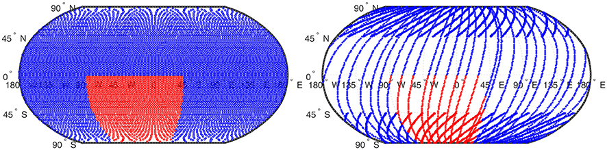
Figure 3. Reuter grid (Left) and scattered grid (Right). The values of the data points in the red area contain an N2S of 5% and the values of the data points in the blue area an N2S of 1% for the local noise scenario.

TABLE 2

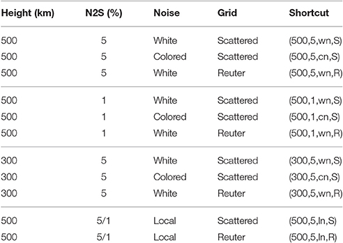
Table 2. Overview of the implemented test cases.

4.4. Regularization Parameters

We constructed the admissible values λ_k for the parameter choice as a monotonically decreasing sequence with 100 values from λ₁ = 1 to ${\lambda }_{100}=10^{-14}$ and a logarithmically equal spacing in the following way

$\begin{array}{ll}{\lambda }_k={\lambda }_0{q}_{\lambda }^k,k\in \left\{1,\dots ,100\right\}.& (33)\end{array}$

Here, λ₀ = 1.3849 and q_λ = 0.7221. The test scenarios are chosen such that the parameter range lies between 1 and 10⁻¹⁴ and includes the optimal parameter away from the boundaries λ₁ and λ₁₀₀. For the choice of the parameters λ_k, we refer to [18, 19].

4.5. Maximal Index

Most parameter choice methods either increase the index k until a certain condition is satisfied or minimize a certain function for all regularization parameters λ, i.e., after our discretization (see Equation 33) they minimize for all k (see Table 1). For some methods like the quasi-optimality criterion, the values of k have to be constrained by a suitable maximal index $\widehat{K}$ which must be chosen such that $k_{opt}<\widehat{K}$. To increase computational efficiency, such a maximal index can be used for other methods as well without changing their performance. As in [18, 19], we define this maximal index by

$\begin{array}{ll}\widehat{K}=max\left\{k|\rho (k)<0.5\rho (\infty )\right\},& (34)\end{array}$

where $\text{E}\Vert x_k-x_k^{\epsilon }{\Vert }^2={\epsilon }^2{\rho }^2(k)$ is the variance of the regularized solution corresponding to noisy data and ε²ρ²(∞) is its largest value. It is well-known that, in the case of white noise, ρ(k) for the Tikhonov-Phillips regularization is generally given by

$\begin{array}{ll}{\rho }^2(k)={\displaystyle \sum _n}{\left(\frac{{\sigma }_n}{{\sigma }_n^2+{\lambda }_k}\right)}^2.& (35)\end{array}$

Since our singular values occur with a multiplicity of 2n + 1 and we restrict our tests to n = 0, …, 100, the sum above in our tests is given by

$\begin{array}{ll}{\rho }^2(k)={\displaystyle \sum _{n=0}^{100}}(2n+1){\left(\frac{{\sigma }_n}{{\sigma }_n^2+{\lambda }_k}\right)}^2.& (36)\end{array}$

For any colored noise, we use the estimate (cf. [19])

$\begin{array}{ll}{\epsilon }^2{\rho }^2(k)\approx 2^{-1}\left|\right|x_{k,1}^{\epsilon }-x_{k,2}^{\epsilon }{\Vert }_{{H}}^2,& (37)\end{array}$

with two independent data sets ${\mathbf{y}}_1^{\epsilon }$, ${\mathbf{y}}_2^{\epsilon }$ for the same regularization parameter λ_k. Note that $x_{k,1}^{\epsilon }$, $x_{k,2}^{\epsilon }$ are the regularized solutions corresponding to the parameter λ_k and the noisy data sets ${\mathbf{y}}_1^{\epsilon }$, ${\mathbf{y}}_2^{\epsilon }$.

5. Comparison of the Methods

For the error comparison, we compute the inefficiency (see Equation 31) in each scenario (see Table 2 for an overview) for each parameter choice method and compare the inefficiencies. We generate 32 data sets for each of the eleven scenarios, i.e., we run each algorithm for 352 times for a single regularization parameter. Figures 4–9 show the inefficiencies, collected based on the parameter choice methods. The red middle band in the box is the median and the red + symbol shows outliers. The boxplots of our results are plotted at a logarithmic scale.

FIGURE 4

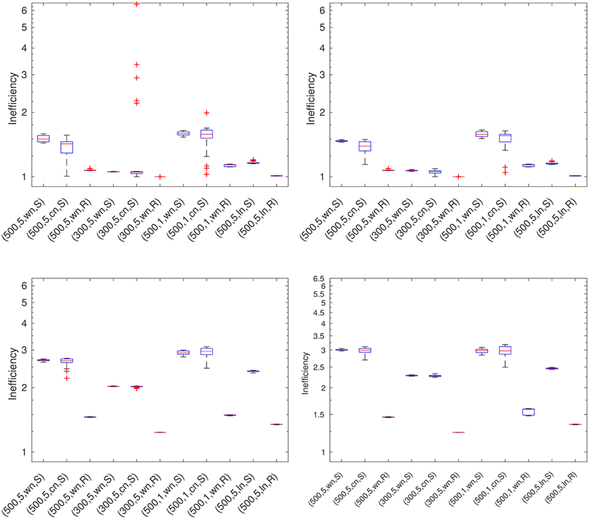
Figure 4. DP for the RFMP (Left-hand top) and the ROFMP (Right-hand top) and TDP for the RFMP (Left-hand bottom) and the ROFMP (Right-hand bottom).

5.1. Discrepancy Principle (DP)

We can see from Figure 4 that the DP leads to results which are in the range from good to acceptable in all test cases. It yields better results with a more uniformly distributed grid.

5.2. Transformed Discrepancy Principle (TDP)

The results for the TDP (see Figure 4) for all test cases are rather poor. We can remark that the results get better with a more uniformly distributed data grid. Furthermore, the colored noise leads to slightly bigger boxes than the white noise.

5.3. Quasi-Optimality Criterion (QOC)

In Figure 5, the inefficiencies of the QOC show that the performance of this method is rather poor. In the case of the Reuter grid, the results reach from good to mediocre in contrast to the scattered grid.

FIGURE 5

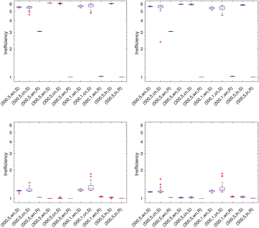
Figure 5. QOC for the RFMP (Left-hand top) and the ROFMP (Right-hand top) and LC for the RFMP (Left-hand bottom) and the ROFMP (Right-hand bottom).

5.4. L-Curve Method (LC)

The LC (see Figure 5) yields good results in all test cases. We can remark that there are a few outliers and bigger boxes for the test cases with colored noise and the scattered grid.

5.5. Extrapolated Error Method (EEM)

The EEM yields acceptable to rather poor results (see Figure 6). We cannot observe any dependency on the grid or the kind of noise related to the acceptable results. Moreover, in the test case with a height of 300 km and an N2S of 5% with colored noise we have some outliers for the RFMP and a large box for the ROFMP.

FIGURE 6

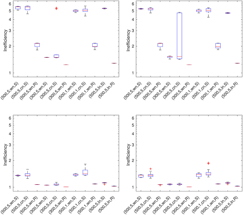
Figure 6. EEM for the RFMP (Left-hand top) and the ROFMP (Right-hand top) and RM for the RFMP (Left-hand bottom) and the ROFMP (Right-hand bottom).

5.6. Residual Method (RM)

The results for the RM (see Figure 6) are good to acceptable in all test cases. We only have a few minor outliers.

5.7. Generalized Maximum Likelihood (GML)

In Figure 7, we can see that the GML leads to acceptable results only in the case of the Reuter grid. In all cases of the scattered grid, its performance is rather bad.

FIGURE 7

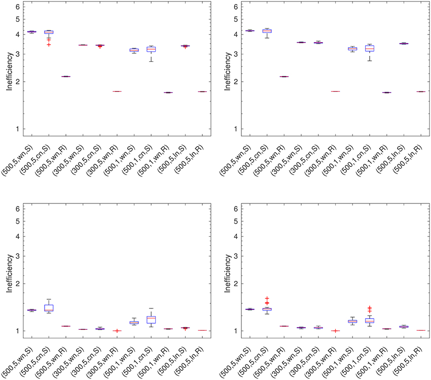
Figure 7. GML for the RFMP (Left-hand top) and the ROFMP (Right-hand top) and GCV for the RFMP (Left-hand bottom) and the ROFMP (Right-hand bottom).

5.8. Generalized Cross Validation (GCV)

From Figure 7, we can observe that the GCV yields good results in all test cases. We only have, in the case of the ROFMP, some minor outliers. It yields the best results with a more regularly distributed data grid.

5.9. Robust Generalized Cross Validation (RGCV)

The RGCV yields good to acceptable results (see Figure 8) which get slightly worse and show a larger variance for a higher N2S or colored noise scenarios.

FIGURE 8

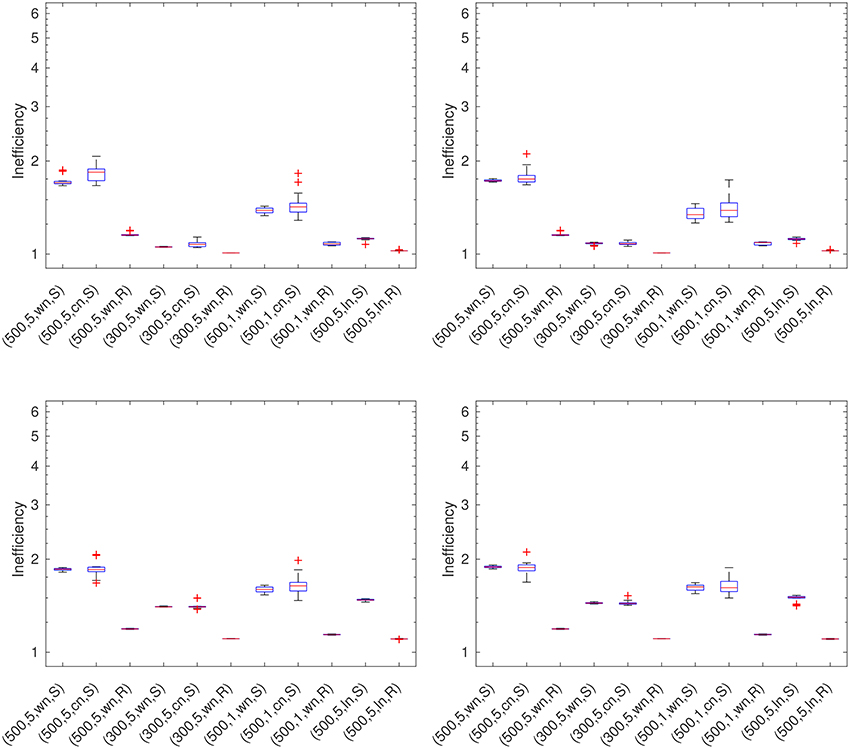
Figure 8. RGCV for the RFMP (Left-hand top) and the ROFMP (Right-hand top) and SRGCV for the RFMP (Left-hand bottom) and the ROFMP (Right-hand bottom).

5.10. Strong Robust Generalized Cross Validation (SRGCV)

The SRGCV (see Figure 8) has good to acceptable results in all the test cases which are a little bit worse than for the RGCV. The Reuter grid leads to good results whereas the scattered grid seems to be more difficult to handle by the method.

5.11. Modified Generalized Cross Validation (MGCV)

The inefficiencies for the MGCV (see Figure 9) for the test cases with white noise and the Reuter grid are good. In particular, in several of the cases with colored noise the boxes are so big that they partially do not fit in the figure. Obviously, we get here a very large distribution of the inefficiencies. These cases seem to be very hard to handle for this method.

FIGURE 9

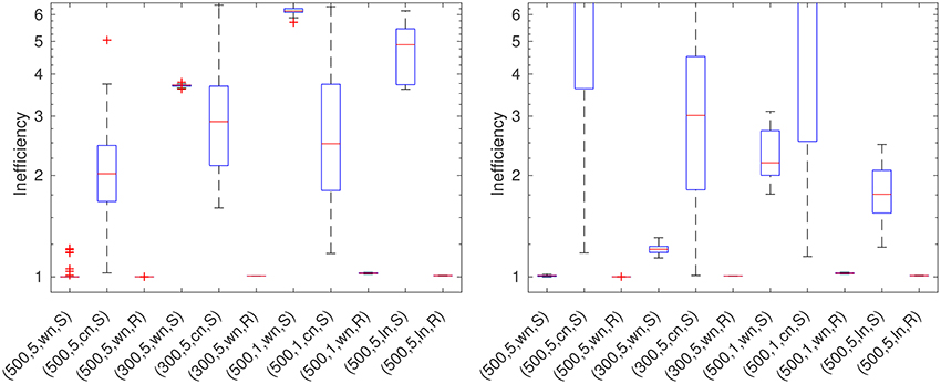
Figure 9. MGCV for the RFMP (Left) and the ROFMP (Right).

5.12. Plots of the Results

In this section, we show briefly the approximations of the gravitational potential which we obtain by the RFMP and the ROFMP for one typical noisy data set considering a good or a rather poor parameter choice.

For the test case (500 km, 5%, colored noise, scattered grid) with α = 0.54 for the AR(1)-process, Figure 10 shows the approximation which we obtain by the RFMP for the optimal regularization parameter λ₂₉ and the difference to the EGM2008 up to degree 100. Figure 11 shows the approximation belonging to the regularization parameter λ₂₂ which is chosen by the GCV. In Figure 12, we can see the approximation belonging to the parameter λ₄₃ which is chosen by the MGCV. We can see that the MGCV chooses the regularization parameter too small and with this choice we obtain a solution which is underregularized. North-South oriented anomalies occur in the reconstruction which appear to be artifacts due to the noise along the simulated satellite tracks. In contrast, the approximation of the potential for the GCV-based parameter is only slightly worse than the result for the optimal parameter.

FIGURE 10

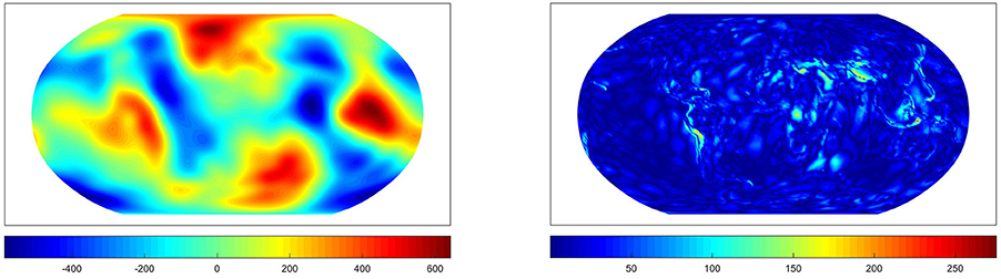
Figure 10. The approximation from the RFMP for the best parameter (Left) and the difference to the EGM2008 up to degree 100 (Right). Values in m²/s².

FIGURE 11

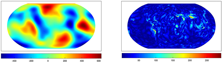
Figure 11. The approximation from the RFMP for the parameter chosen by the GCV (Left) and the difference to the EGM2008 up to degree 100 (Right). Values in m²/s². The inefficiency amounts to 1.16.

FIGURE 12

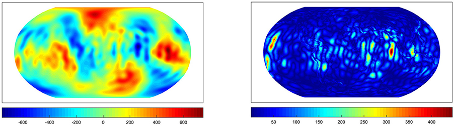
Figure 12. The approximation from the RFMP for the parameter chosen by the MGCV (Left) and the difference to the EGM2008 up to degree 100 (Right). Values in m²/s². The inefficiency amounts to 2.29.

Furthermore, we show the same test case as above but with the approximation from the ROFMP with α = 0.56 in the AR(1)-process. Figure 13 shows the approximation for the optimal parameter λ₂₉ and the difference to EGM2008 up to degree 100. In Figure 14, we see the approximation which belongs to the parameter λ₂₂ which is chosen by the GCV. Figure 15 shows the approximation with the regularization parameter λ₉ which is chosen by the GML.

FIGURE 13

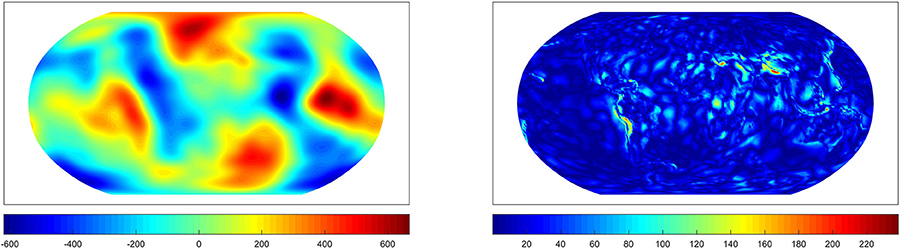
Figure 13. The approximation from the ROFMP for the best parameter (Left) and the difference to the EGM2008 up to degree 100 (Right). Values in m²/s².

FIGURE 14

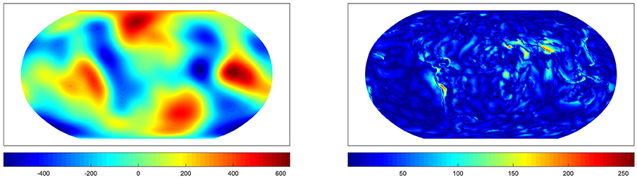
Figure 14. The approximation from the ROFMP for the parameter chosen by the GCV (Left) and the difference to the EGM2008 up to degree 100 (Right). Values in m²/s². The inefficiency amounts to 1.14.

FIGURE 15

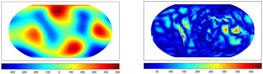
Figure 15. The approximation from the ROFMP for the parameter chosen by the GML (Left) and the difference to the EGM2008 up to degree 100 (Right). Values in m²/s². The inefficiency amounts to 3.03.

Here, the GML chooses a regularization parameter which is too large, that means our approximation is overregularized. We get less information and details about the gravitational potential. Essential details such as signals due to the Andes or the region around Indonesia occur in the difference plot—much stronglier than for the other examples. Again the parameter choice of the GCV yields a good approximation for the gravitational potential.

Finally, Figures 16, 17 show the difference $\Vert x-x_k^{\epsilon }{\Vert }_{L2(\Omega )}$ between the original solution (i.e., EGM2008 up to degree 100) and the approximation $x_k^{\epsilon }$ obtained for the different regularization parameters which were chosen by the considered strategies. The horizontal axis states the index k of the regularization parameter λ_k. The plots refer to the same scenario as Figures 10–15. The arrows show the parameters which are chosen by the methods. The diagrams confirm our observations that the GCV and the LC yield parameters which are closest to the (theoretical) optimal parameter. We obtain almost equally good results for the DP, the RM and the RGCV.

FIGURE 16

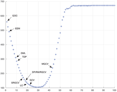
Figure 16. The horizontal axis states the index k of the regularization parameter and the vertical axis shows $\Vert x-x_k^{\epsilon }{\Vert }_{L2(\Omega )}$ for the RFMP.

FIGURE 17

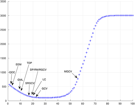
Figure 17. The horizontal axis states the index k of the regularization parameter and the vertical axis shows $\Vert x-x_k^{\epsilon }{\Vert }_{L2(\Omega )}$ for the ROFMP.

6. Conclusion and Outlook

We tested parameter choice methods for the regularized (orthogonal) functional matching pursuit (RFMP/ROFMP) in the context of the downward continuation problem. For the evaluation of the parameter choice methods, we constructed eleven different test cases with different satellite heights, data grids, noise types and noise-to-signal ratios (see Table 2) for the RFMP and ROFMP. For each test case, we generated 32 noisy data sets. Altogether we ran each algorithm for 352 data sets and for each data set for 100 different regularization parameters, that means each algorithm was applied 35,200 times.

Our study shows that the GCV, the LC and the RM yield the best results in all test cases, where the RGCV and the SRGCV are almost equally good. The DP provides good to acceptable results. The performance of the QOC seriously depends on the data grid, that means a less regularly distributed grid does not lead to good results. In our experiments, the QOC had good results with the Reuter grid in most cases. The MGCV also obtains both good and rather poor results in dependency on the grid and kind of noise we used. Here, the irregularly distributed scattered grid and the colored noise did not yield good results. At last, the TDP, the EEM and the GML did not always lead to good results in our test cases.

Note that not all results can be explained since some methods are still of rather heuristic nature and convergence analysis does not exist even for simpler regularizations such as ordinary Tikhonov regularization (see [18, 19] for an overview). Often these methods are formulated and investigated without considering discretization and data distribution issues. As our study shows, not all of them transfer well from the continuous to the discrete setting. It should also be noted that the GCV is known to work very well with data afflicted by white noise, but cannot deal well with colored noise. Our colored noise scenario using the AR(1)-process might be too mild to show these effects. The variants of the GCV, i.e., RGCV, SRGCV, and MGCV, use their tuning parameter to trade a little bit of performance in the case of white noise problems for a large improvement in the colored noise case. There might still be the chance for some improvements using another tuning parameter than in [18, 19].

We want to remark that in average our results were better than in [18, 19] for all methods. Some possible reasons for that can be: the colored noise in our test cases was different and maybe easier to handle for the methods than in the two papers, because we only had an AR(1)-process. There is a further difference to the other cases in relation to the problem itself. Here we had a data grid given which corresponds to a spatial discretization of the problem. Furthermore, the RFMP and the ROFMP are iterative methods and use stopping criteria which are also some kind of regularization. Since we stop the algorithm at a certain point we do not obtain the approximation of the potential in the limit. For these reasons, the outcomes of our experiments and of those in [18, 19] are not really comparable.

The purpose of this paper is to provide a first guideline for the parameter choice for the RFMP and the ROFMP. Certainly, further experiments should be designed in the future. Maybe, the distribution of our regularization parameters λ_k could be improved such that the relevant parameters themselves are not too wide apart. Perhaps, the interval from 1 to 10⁻¹⁴ should be chosen smaller such that the parameters are closer together.

Moreover, note that we have not addressed the stopping criterion of the RFMP and the ROFMP here, though the maximal number of iterations is another regularization parameter. A detailed investigation of this criterion is a subject for future research. Furthermore, an enhancement could be the extension of the dictionary to localized trial functions. In addition, the generation of the colored noise can, for example, use an AR(k)-process for k > 1 or completely different types of noise can be considered. Finally, we can test other tuning parameters for the methods as far as these are required. Besides, it is possible that the performance of the investigated parameter choice methods in the RFMP/ROFMP depends on the considered inverse problem.

Author Contributions

All authors listed, have made substantial, direct and intellectual contribution to the work, and approved it for publication.

Conflict of Interest Statement

The authors declare that the research was conducted in the absence of any commercial or financial relationships that could be construed as a potential conflict of interest.

References

1. Ilk KH, Flury J, Rummel R, Schwintzer P, Bosch W, Haas C, et al. Mass Transport and Mass Distribution in the Earth System: Contribution of the New Generation of Satellite Gravity and Altimetry Missions to Geosciences. GOCE-Projektbüro TU München, GeoForschungsZentrum Potsdam (2004). Availbale online at: http://gfzpublic.gfz-potsdam.de/pubman/faces/viewItemOverviewPage.jsp?itemId=escidoc:231104:1 (Accessed March 10, 2017).

Google Scholar

2. Kusche J, Klemann V, and Sneeuw N Mass distribution and mass transport in the Earth system: recent scientific progress due to interdisciplinary research. Surv Geophys. (2014) 35:1243–49. doi: 10.1007/s10712-014-9308-9

CrossRef Full Text | Google Scholar

3. Drinkwater MR, Haagmans R, Muzi D, Popescu A, Floberghagen R, Kern M, and et al. The GOCE gravity mission: ESA's first core explorer. In: Proceedings of the 3rd GOCE User Workshop, Vol. SP-627. Frascati: ESA Special Publication (2006). p. 1–8.

Google Scholar

4. Pail R, Goiginger H, Schuh WD, Höck E, Brockmann JM, Fecher T, and et al. Combined satellite gravity field model GOCO01S derived from GOCE and GRACE. Geophys Res Lett. (2010) 37:L20314. doi: 10.1029/2010GL044906

CrossRef Full Text | Google Scholar

5. Reigber C, Balmino G, Schwintzer P, Biancale R, Bode A, Lemoine JM, et al. New global gravity field models from selected CHAMP data sets. In: Reigber C, Lühr H, Schwintzer P, editors. First CHAMP Mission Results for Gravity, Magnetic and Atmospheric Studies. Berlin; Heidelberg: Springer (2003). p. 120–7. doi: 10.1007/978-3-540-38366-6_18

CrossRef Full Text | Google Scholar

6. Tapley BD, Bettadpur S, Watkins M, and Reigber C. The gravity recovery and climate experiment: mission overview and early results. Geophys Res Lett. (2004) 31:L09607. doi: 10.1029/2004GL019920

CrossRef Full Text | Google Scholar

7. Freeden W, Michel V. Multiscale Potential Theory. With Applications to Geoscience. Boston, MA: Birkhäuser (2004). doi: 10.1007/978-1-4612-2048-0

CrossRef Full Text | Google Scholar

8. Schneider F. Inverse Problems in Satellite Geodesy and Their Approximation in Satellite Gradiometry. Ph.D. thesis, Geomathematics Group, Department of Mathematics, University of Kaiserslautern. Aachen: Shaker (1997).

9. Freeden W, and Gutting M. Special Functions of Mathematical (Geo-) physics. Basel: Birkhäuser (2013). doi: 10.1007/978-3-0348-0563-6

CrossRef Full Text | Google Scholar

10. Michel V. Lectures on Constructive Approximation – Fourier, Spline, and Wavelet Methods on the Real Line, the Sphere, and the Ball. New York, NY: Birkhäuser (2013). doi: 10.1007/978-0-8176-8403-7

CrossRef Full Text | Google Scholar

11. Müller C. Spherical Harmonics. Berlin; Heidelberg: Springer (1966). doi: 10.1007/BFb0094775

PubMed Abstract | CrossRef Full Text

12. Pavlis NK, Holmes SA, Kenyon SC, Factor JK. The development and evaluation of the Earth Gravitational Model 2008 (EGM2008). J Geophys Res. (2012) 117:B04406. doi: 10.1029/2011jb008916

CrossRef Full Text | Google Scholar

13. Telschow R. An Orthogonal Matching Pursuit for the Regularization of Spherical Inverse Problems. Ph.D. thesis, Geomathematics Group, Department of Mathematics, University of Siegen. Munich: Dr. Hut (2015).

14. Mallat SG, and Zhang Z. Matching pursuits with time-frequency dictionaries. IEEE Trans Signal Process. (1993) 41:3397–415. doi: 10.1109/78.258082

CrossRef Full Text | Google Scholar

15. Pati YC, Rezaiifar R, and Krishnaprasad PS. Orthogonal matching pursuit: recursive function approximation with applications to wavelet decomposition. In: Asimolar Conference on Signals, Systems and Computers. Vol. 1 of IEEE Conference Publications. Los Alamitos (1993). p. 40–44. doi: 10.1109/ACSSC.1993.342465

CrossRef Full Text | Google Scholar

16. Vincent P, and Bengio Y. Kernel matching pursuit. Mach Learn. (2002) 48:165–87. doi: 10.1023/A:1013955821559

CrossRef Full Text | Google Scholar

17. Engl HW, Hanke M, and Neubauer A. Regularization of Inverse Problems. Dordrecht: Kluwer (1996). doi: 10.1007/978-94-009-1740-8

CrossRef Full Text | Google Scholar

18. Bauer F, Gutting M, and Lukas MA. Evaluation of parameter choice methods for the regularization of ill-posed problems in geomathematics. In: Freeden W, Nashed MZ, Sonar T, editors. Handbook of Geomathematics. 2nd Edn. Berlin; Heidelberg: Springer (2015). p. 1713–74. doi: 10.1007/978-3-642-54551-1_99

CrossRef Full Text | Google Scholar

19. Bauer F, and Lukas MA. Comparing parameter choice methods for regularization of ill-posed problems. Math Comput Simul. (2011) 81:1795–841. doi: 10.1016/j.matcom.2011.01.016

CrossRef Full Text | Google Scholar

20. Fischer D. Sparse Regularization of a Joint Inversion of Gravitational Data and Normal Mode Anomalies. Ph.D. thesis, Geomathematics Group, Department of Mathematics, University of Siegen. Munich: Dr. Hut (2011).

21. Fischer D, and Michel V. Sparse regularization of inverse gravimetry—case study: spatial and temporal mass variations in South America. Inverse Prob. (2012) 28:065012. doi: 10.1088/0266-5611/28/6/065012

CrossRef Full Text | Google Scholar

22. Michel V. RFMP – an iterative best basis algorithm for inverse problems in the geosciences. In: Freeden W, Nashed MZ, Sonar T, editors. Handbook of Geomathematics, 2nd Edn. Berlin; Heidelberg: Springer (2015). p. 2121–47. doi: 10.1007/978-3-642-54551-1_93

CrossRef Full Text | Google Scholar

23. Michel V, and Telschow R. A non-linear approximation method on the sphere. GEM Int J Geomath. (2014) 5:195–224. doi: 10.1007/s13137-014-0063-3

CrossRef Full Text | Google Scholar

24. Michel V, and Telschow R. The regularized orthogonal functional matching pursuit for ill-posed inverse problems. SIAM J Numer Anal. (2016) 54:262–87. doi: 10.1137/141000695

CrossRef Full Text | Google Scholar

25. Michel V, and Orzlowski S. On the convergence theorem for the Regularized Functional Matching Pursuit (RFMP) algorithm. GEM Int J Geomath. (2017). doi: 10.1007/s13137-017-0095-6. [Epub ahead of Print].

CrossRef Full Text | Google Scholar

26. Freeden W, Gervens T, and Schreiner M. Constructive Approximation on the Sphere with Applications to Geomathematics. Oxford: Oxford University Press (1998).

27. Morozov VA. On the solution of functional equations by the method of regularization. Sov Math Dokl. (1966) 7:414–7.

28. Morozov VA. Methods for Solving Incorrectly Posed Problems. New York, NY: Springer (1984). doi: 10.1007/978-1-4612-5280-1

CrossRef Full Text | Google Scholar

29. Phillips DL. A technique for the numerical solution of certain integral equations of the first kind. J Assoc Comput Mach. (1962) 9:84–97. doi: 10.1145/321105.321114

CrossRef Full Text | Google Scholar

30. Raus T. An a posteriori choice of the regularization parameter in case of approximately given error bound of data. In: Pedas A, editor. Collocation and Projection Methods for Integral Equations and Boundary Value Problems. Tartu: Tartu University (1990). p. 73–87.

31. Raus T. About regularization parameter choice in case of approximately given error bounds of data. In: Vainikko G, editor. Methods for Solution of Integral Equations and Ill-posed Problems. Tartu: Tartu University (1992). p. 77–89.

32. Tikhonov AN, and Arsenin VY. Solutions of Ill-Posed Problems. New York, NY: Wiley (1977).

Google Scholar

33. Tikhonov AN, and Glasko VB. Use of the regularization method in non-linear problems. USSR Comput Math Math Phys. (1967) 5:93–107. doi: 10.1016/0041-5553(65)90150-3

CrossRef Full Text | Google Scholar

34. Hansen PC. Analysis of discrete ill-posed problems by means of the L-curve. SIAM Rev. (1992) 34:561–80. doi: 10.1137/1034115

CrossRef Full Text | Google Scholar

35. Hansen PC. Rank-deficient and Discrete Ill-posed Problems. Numerical Aspects of Linear Inversion. Philadelphia, PA: SIAM (1998). doi: 10.1137/1.9780898719697

CrossRef Full Text | Google Scholar

36. Hansen PC, and O'Leary DP. The use of the L-curve in the regularization of discrete ill-posed problems. SIAM J Sci Comput. (1993) 14:1487–503. doi: 10.1137/0914086

CrossRef Full Text | Google Scholar

37. Brezinski C, Rodriguez G, and Seatzu S. Error estimates for linear systems with applications to regularization. Numer Algorithms. (2008) 49:85–104. doi: 10.1007/s11075-008-9163-1

CrossRef Full Text | Google Scholar

38. Brezinski C, Rodriguez G, and Seatzu S. Error estimates for the regularization of least squares problems. Numer Algorithms. (2009) 51:61–76. doi: 10.1007/s11075-008-9243-2

CrossRef Full Text | Google Scholar

39. Bauer F, Mathé P. Parameter choice methods using minimization schemes. J Complex. (2011) 27:68–85. doi: 10.1016/j.jco.2010.10.001

CrossRef Full Text | Google Scholar

40. Wahba G. A comparison of GCV and GML for choosing the smoothing parameter in the generalized spline smoothing problem. Ann Stat. (1985) 13:1378–402. doi: 10.1214/aos/1176349743

CrossRef Full Text | Google Scholar

41. Wahba G. Practical approximate solutions to linear operator equations when the data are noisy. SIAM J Numer Anal. (1977) 14:651–67. doi: 10.1137/0714044

CrossRef Full Text | Google Scholar

42. Lukas MA. Robust generalized cross-validation for choosing the regularization parameter. Inverse Prob. (2006) 22:1883–902. doi: 10.1088/0266-5611/22/5/021

CrossRef Full Text | Google Scholar

43. Robinson T, Moyeed R. Making robust the cross-validatory choice of smoothing parameter in spline smoothing regression. Commun Stat Theory Methods (1989) 18:523–39. doi: 10.1080/03610928908829916

CrossRef Full Text | Google Scholar

44. Lukas MA. Strong robust generalized cross-validation for choosing the regularization parameter. Inverse Prob. (2008) 24:034006. doi: 10.1088/0266-5611/24/3/034006

CrossRef Full Text | Google Scholar

45. Cummins DJ, Filloon TG, Nychka D. Confidence intervals for nonparametric curve estimates: toward more uniform pointwise coverage. J Am Stat Assoc. (2001) 96:233–46. doi: 10.1198/016214501750332811

CrossRef Full Text | Google Scholar

46. Vio R, Ma P, Zhong W, Nagy J, Tenorio L, Wamsteker W. Estimation of regularization parameters in multiple-image deblurring. Astron Astrophys. (2004) 423:1179–86. doi: 10.1051/0004-6361:20047113

CrossRef Full Text | Google Scholar

47. Wahba G. Spline Models for Observational Data. Philadelphia, PA: SIAM (1990). doi: 10.1137/1.9781611970128

CrossRef Full Text | Google Scholar

48. Reuter R. Integralformeln der Einheitssphäre und harmonische Splinefunktionen. Ph.D. thesis. Aachen: RWTH Aachen (1982).

49. Brockwell PJ, Davis RA. Introduction to Time Series and Forecasting. 2nd Edn. New York, NY: Springer (2002). doi: 10.1007/b97391

CrossRef Full Text | Google Scholar

50. Heirtzler JR. The future of the South Atlantic anomaly and implications for radiation damage in space. J Atmos Sol Terr Phys. (2002) 64:1701–8. doi: 10.1016/S1364-6826(02)00120-7

CrossRef Full Text | Google Scholar