Sequences by Metastable Attractors: Interweaving Dynamical Systems and Experimental Data

1. Introduction

Metastable states (MS) and heteroclinic orbits (HO) are prevalent in various biological and physical systems with essentially separated time scales. A MS can be characterized as a domain in a system's phase space with relatively large dwell time and slow evolution that is separated from another MS through a fast transient regime. Such slow phases may be constant states, oscillatory states or even parts of chaotic attractors [1]. In general, one may say that MS are quasistationary states with an attractive input channel and a repelling output channel, the simplest examples are hyperbolic saddles that may be connected along their stable and unstable manifolds, thus forming a heteroclinic orbit (HO) [2]. In case of dispersive saddles with one-dimensional unstable manifolds, a HO may assume the form of a stable heteroclinic sequence (SHS) [3, 4] or a heteroclinic network [5]. In the following, we will investigate a set of several of such connected dispersive saddles and call it SHS in accordance to Rabinovich et al. [4].

Well-known examples of such sequences are the solution of the generalized Lotka-Volterra model for the population of species [3, 6], the Küppers-Lortz instability occurring at the onset of convection in a Rayleigh-Benard experiment in the presence of rotation [7, 8] or even the well-known chaotic Lorenz attractor [9] where the two butterfly wings represent MS. In recent years, several experimental studies of biological systems have revealed that the systems' activities evolve between some equilibria [10–12]. Such HOs between MS may occur in neural responses in the insect olfactory bulb [13], in bird songs [14], in human scalp brain activity at rest [15], during cognitive tasks [16, 17], in schizophrenia [18] and during emergence from unconsciousness [19]. HOs are even hypothesized to represent a coding scheme in neural systems [1] termed chaotic itinerancy in this context [20, 21].

To explore the nature and underlying mechanisms of HOs, it is necessary to identify their constituent MS and heteroclinic connections between them and to develop models for describing them analytically. These models give insights into possible underlying dynamics. For instance, in a previous series of studies, sequences of MS have been identified in encephalographic data during cognitive tasks [17] and in early human auditory processing [22]. Since the brain processes stimuli under experimental conditions from a starting state at rest and returns to a resting state, sequences of MS in a heteroclinic network represent HOs [5]. Studies on the dimensionality of the system dynamics of these MS have revealed that the data close to MS can be described analytically by low-dimensional dynamical systems [22], whereas the transitions between MS are high-dimensional. In the view of the theory of complex systems [23, 24] such low-dimensional dynamics reflects a certain order or self-organization in the underlying system whereas high-dimensional transitions may be viewed as being unordered. Moreover, the MS show very good accordance in phase space location, onset time and duration to so-called event-related potentials (ERP) in case of cognitive tasks or evoked potentials (EP) in case of early auditory processing. These components are well-known to reflect neural processing mechanisms [22, 25]. Summarizing, brain signals may exhibit HO, processing information in steps of low-dimensional self-organized MS [5].

To understand HO observed in experimental data, we propose a sequence of interweaving data analysis and modeling techniques. Since a HO exhibits a temporal sequence of MS, in a first step these states are extracted by data analysis techniques identifying their location in phase space, their onset times and their durations as essential features [8, 12, 22, 25–27]. These features are assumed to fully describe the HO and typically are rather invariant in experimental repetitions. For instance, in human cognitive neuroscience experiments measuring electroencephalographic activity (EEG), these MS are the so-called event-related components reflecting specific neural processing tasks during cognition [22, 25]. For bird songs, MS are firing states of neural cell assemblies [14].

The corresponding data analysis methods are based on certain model assumptions on the underlying dynamics. Some methods separate MSs from transients by machine learning techniques while neglecting the latter [8, 22]. This implies a clear separation of time scales between slow MS and fast transients. A consequence is that measured data are assumed to accumulate strongly in MS and are sparse during transients. Other methods consider MS as recurrence domains and transients between them as non-recurrent regimes. Then the recurrent and non-recurrent states partition the underlying phase space into disjoint cells, thereby yielding a symbolic dynamics where all non-recurrent transients are mapped to a single symbol, i.e., they are undistinguishable [12, 26, 27]. To determine such a symbolic dynamics, an underlying stochastic model on the temporal distribution of MS is mandatory.

Once the sequence of MS has been identified as principle features of the measured data, their HO can be modeled as a dynamical system. The model features are the spatial localization, the onset time and the duration of each MS. To this end, we choose the dynamic skeleton of a sequence of MS and insert the corresponding features. The resulting model represents a combination of optimally extracted experimental data and a dynamical model.

The present work illustrates a certain combination of system identification and modeling techniques to extract sequences of MS in HOs. Parts of this combination have been developed in recent years while we present novel extensions that improve the identification of MS in experimental data under different experimental conditions. In the application, we focus on brain signals but the methodology may be applied easily to experimental data measured in other physical, biological, or geo-systems.

2. Materials and Methods

The following sections illustrate in detail both a data analysis method for the extraction of MS features and a model approach to describe the HO of experimental data mathematically.

2.1. Identification of HO: The Recurrence Structure Analysis

Let us consider a set of discretely sampled trajectories $\left\{{(x_t^{(c)})}_{1\le t\le T}|t,T,c\in \mathbb{N}\right\}$ in the phase space X of a dynamical system with sampling time t. The system depends on a (discretized) control parameter c ∈ ℕ (hence taken from natural numbers, here), indicating several experimental conditions. T denotes the number of samples and X is a subset of ℝⁿ. An example might be a multivariate measured signal with dimension n. Note that for univariate time series, X can be reconstructed through phase space embedding [28] or, more recently, through spectral embedding techniques [29, 30]. For a given c ∈ ℕ the system's realization $(x_t^{(c)})$ is a function from the index set T = {t|1 ≤ t ≤ T} into X, i.e., $(x_t^{(c)})$ ∈ X^T.

Starting point of the (symbolic) recurrence structure analysis (RSA) is Poincaré's famous recurrence theorem [31] stating that almost all trajectories starting in a “ball” B_ε(x₀) of radius ε > 0 centered at an initial condition x₀ ∈ X return infinitely often to B_ε(x₀) as time elapses, when the dynamics possesses an invariant measure and is restricted to a finite portion of phase space. For time-discrete dynamical systems, these recurrences can be visualized by means of Eckmann et al.'s [32] recurrence plot (RP) technique where the element

$\begin{array}{cc}{R}_{ij}=\{\begin{array}{ll}1\hfill & \text{if}{x}_j\in B_{\epsilon }(x_i)\hfill \\ 0\hfill & \text{else}\hfill \end{array}.& \left(1\right)\end{array}$

of the recurrence matrix R = (R_ij) is unity if the state x_j at time j belongs to an ε-ball

$\begin{array}{cc}{B}_{\epsilon }(x_i)=\{x\in X|d(x,x_i)<\epsilon \}& \left(2\right)\end{array}$

centered at state x_i at time i and zero otherwise [32, 33]. Here d: X × X → ℝ⁺ denotes some distance function, which is a metric in general.

Recurrent events (R_ij = 1) of the dynamics lead to intersecting ε-balls B_ε(x_i) ∩ B_ε(x_j) ≠ ∅ which can be merged together into equivalence classes of phase space X. By merging balls together into a set A_j = B_ε(x_i) ∪ B_ε(x_j) when states x_i and x_j are recurrent and when i > j, we simply replace the larger time index i in the recurrence plot R by the smaller one j, symbolized as a rewriting rule i → j of a recurrence grammar [12, 26, 27].

Applying the recurrence grammar that corresponds to a recurrence plot R for given ball size ε recursively to the sequence of sampling times r_i = i with 1 ≤ i ≤ T yields a segmentation of the system's multivariate time series into discrete states s_i = k, i.e., a symbolic dynamics based on a finite partition ${P}=\left\{A_k\subset X|0\le k\le m_a\right\}$ of the phase space X into m_a + 1 disjoint sets A_k, such that x_i ∈ A_k. In this representation the distinguished state 0 captures all transients, while m_a is the number of detected MS [12].

The results of the RSA and the obtained symbolic dynamics depend heavily on the parameter ε that defines the ball size of recurrent events. For finding an optimal partition and hence an optimal value for ε, beim Graben and Hutt [12, 26] and beim Graben et al. [27] have suggested several entropy-based criteria. To gain an optimal segmentation, the idea is to assume an underlying stochastic model for the symbolic sequences. Then the optimal segmentation is as close as possible to the model under consideration. For instance, assuming a uniform probability distribution of symbols, the optimal value ε maximizes the entropy of the states [26]. Here, we employ the most recently suggested Markov optimization criterion [27], maximizing a utility function

$\begin{array}{cc}u(\epsilon )=\frac{1}{n+2}\left[\text{tr}P(\epsilon )+h_r(\epsilon )+h_c(\epsilon )\right]& \left(3\right)\end{array}$

for a Markov transition matrix P estimated from the bi-gram distribution of the symbolic sequence s. Here

$\begin{array}{cc}\begin{array}{l}{h}_r=-\frac{1}{\log (n-1)}{\displaystyle \sum _{j=1}^{n-1}p{\prime }_{0j}\log p{\prime }_{0j}}\\ h_c=-\frac{1}{\log (n-1)}{\displaystyle \sum _{i=1}^{n-1}p{\prime }_{i0}\log p{\prime }_{i0}}\end{array}& \left(4\right)\end{array}$

are renormalized entropies with $p_{0j}^{\prime }=p_{0j}/\sum _{j=1}^{n-1}{p}_{0j}$ for the first row and $p_{i0}^{\prime }=p_{i0}/\sum _{i=1}^{n-1}{p}_{i0}$ for the first column of P. The transition rates p_ij in P are estimated for each value of ε. The parameter ε* maximizing u(ε) is then the optimal threshold for which the recurrence structure detected from the time series mostly resembles an unbiased Markov chain model.

Applying the RSA to the time series $(x_i^{(c)})$ ∈ X^T for several experimental conditions separately yields a symbolic sequence s^(c) for each condition. Each sequence is based on a unique phase space partition ${{P}}^{(c)}=\left\{A_k^{(c)}\subset X|0\le k\le m^{(c)}\right\}$, c ∈ ℕ. In order to unify such different descriptions for all experimental conditions within a common picture based on a single partition, beim Graben and Hutt [12] suggested a recursive Hausdorff clustering method. As this method turned out to be rather time consuming in practical applications, we present a substantially improved non-recursive algorithm for the alignment of multiple realizations of dynamical system's trajectories in the sequel.

For this aim let us assume two experimental conditions, i.e., c = 1, 2, without loss of generality. Our new, more parsimonious, approach is introduced by a recoding of the symbolic sequences s^(c) for c > 1 based on the symbolic sequence s⁽¹⁾. Thus we leave the symbols for the first condition (c = 1) unchanged but alter the symbols for the second condition through an additive constant, i.e.,

$\begin{array}{cc}{q}_i^{(c)}=\{\begin{array}{ll}{s}_i^{(c)}+(c-1)T\hfill & \text{if}{s}_i^{(c)}\ne 0\hfill \\ 0\hfill & \text{else}\hfill \end{array}& \left(5\right)\end{array}$

with T as the length of each sequence s^(c). This is possible as symbols are simply represented as integer numbers in our framework¹. Note that the “transient symbol” 0 is not affected by the recoding, thereby merging together all transients across conditions.

Afterwards, both the original time series $(x_i^{(c)})$ ∈ X^T and their recoded segmentations q^(c) are concatenated into two long series

$\begin{array}{cc}\begin{array}{l}{\left({\xi }_i\right)}_{1\le i\le 2T}=\left(x_1^{(1)}\dots x_T^{(1)}{x}_1^{(2)}\dots x_T^{(2)}\right)\\ {\left({\eta }_i\right)}_{1\le i\le 2T}=\left(q_1^{(1)}\dots q_T^{(1)}{q}_1^{(2)}\dots q_T^{(2)}\right)\end{array}& \left(6\right)\end{array}$

such that the concatenation products are now functions from 2T = {t|1 ≤ t ≤ 2T} into X, i.e., (ξ_i) ∈ X^2T.

From these data we gather all sampling points that belong to the same phase space cell B_k labeled by the symbol k, i.e., B_k = {ξ_i|η_i = k} ⊂ X. The family of these m_b sets is in general not a partition, but certainly a covering ${Q}=\left\{B_k\subset X|0\le k\le m_b\right\}$ of X. From the members of ${Q}$ we calculate the pairwise Hausdorff distances [34]

$\begin{array}{cc}{D}_{ij}=\max \left\{\max \right\{\delta (y,B_j)|y\in B_i\},\max \{\delta (y,B_i)|y\in B_j\left\}\right\}& \left(7\right)\end{array}$

where

$\begin{array}{cc}\delta (x,A)=\min \{d(x,y)|y\in A\}& \left(8\right)\end{array}$

measures the “distance” of the point x from the compact set A ⊂ X. The Hausdorff distance of two overlapping compact sets vanishes.

Now we proceed as in the previous approach by beim Graben and Hutt [12]: From the pairwise Hausdorff distances (7) we compute a θ-similarity matrix S with elements

$\begin{array}{cc}{S}_{ij}=\{\begin{array}{ll}1\hfill & \text{if}{D}_{ij}<\theta \hfill \\ 0\hfill & \text{else}\hfill \end{array}& \left(9\right)\end{array}$

which consists of zeros and ones as the recurrence matrix R from Equation (1). Therefore, S can also be regarded as a recurrence grammar, for merging the members of ${Q}$ into new partition cells by rewriting large indices of B_i through smaller ones from B_j (i > j) when they are θ-similar (S_ij = 1). The result of the Hausdorff clustering is a unique new partition ${R}=\left\{C_k\subset X|0\le k\le m_c\right\}$ entailing a symbolic dynamics p^(c) for both conditions based on the same symbolic repertoire.

For the application to the ERP data shown below, we chose a rather small similarity distance of θ = 0.25 in order to identify at least the pre-stimulus domain across conditions.

In the view of our subsequent modeling in Section 2.2, recall that the found segments of the RSA are MS in phase space. Therefore, we compute their centers of gravity as time-averaged topographies

$\begin{array}{cc}{v}_k=\frac{1}{T_k}{\displaystyle \sum _{i\forall p_i=k}{x}_i}& \left(10\right)\end{array}$

where x_i ∈ C_k and T_k is the number of samples in C_k.

2.2. Construction of SHS: Neural Fields

The recurrence structure analysis, Section 2.1, of the measured data yields a sequential dynamics for each experimental condition. From our present analysis Section 3.1 let us assume that we obtain a total number of m_c MS after Hausdorff clustering. For illustration reasons (cf. Section 3), we assume m_c = 8 and we gain the following pattern sequences

$\begin{array}{cc}\begin{array}{l}{V}^{(1)}=(v_1,v_2,v_3,v_4,v_5,v_6)\\ V^{(2)}=(v_1,v_2,v_7,v_3,v_6,v_8)\end{array}& \left(11\right)\end{array}$

forming n × l matrices for the n-dimensional EEG observation space with l = 6 MS per condition. The spatial patterns result from an underlying system dynamics, that exhibits a HO. To gain deeper insight into the system dynamics that generates the SHS gained experimentally, a second step aims to derive the underlying system model dynamics. To this end, we identify the MS as equilibria in the underlying dynamical system model. Each pattern, i.e., column of V^(c) can be seen as a spatial discretization of a continuous spatial neural field v(x) [35] serving as a saddle in a heteroclinic sequence of field activations [36–38].

In the following we use the findings of beim Graben and Hutt [36] and Schwappach et al. [38] for the modeling of the SHS dynamics by means of heterogeneous neural fields. Our starting point is the Amari equation

$\begin{array}{cc}\tau \frac{\partial u(x,t)}{\partial t}+u(x,t)={\displaystyle {\int }_{\Omega }(x,y)f(u(y,t))\text{d}y}& \left(12\right)\end{array}$

describing the evolution of neural activity u(x, t) at site x ∈ Ω ⊂ ℝ^b and time t [39]. Here, Ω is a b-dimensional manifold, representing neural tissue. Furthermore, w(x, y) is the synaptic weight kernel, and f is a sigmoidal activation function, often taken as f(u) = 1/(1 + exp(− β (u − θ))), with gain β > 0, and threshold θ > 0. The characteristic time constant τ will be deliberately absorbed by the kernel w(x, y) in the sequel.

The metastable segmentation patterns of the RSA (11) are interpreted as stationary states, v(x), of the Amari equation that are connected along their stable and unstable directions, thereby forming a stable heteroclinic sequence (SHS: 3, 4). Such SHS are examples of heteroclinic orbits connecting different equilibria. Let {v_k(x)}, 1 ≤ k ≤ n be a collection of MS which we assume to be linearly independent. Then, this collection possesses a biorthogonal system of adjoints $\left\{v_k^{+}(x)\right\}$ obeying

$\begin{array}{cc}{\displaystyle {\int }_{\Omega }{v}_j^{+}}(x)v_k(x)\text{ d}x={\delta }_{jk}.& \left(13\right)\end{array}$

For the particular case of Lotka-Volterra neural populations, described by activities ξ_k(t),

$\begin{array}{cc}\frac{\text{d}{\xi }_k}{\text{d}t}={\xi }_k\left({\sigma }_k-{\displaystyle \sum _{j=1}^n{\rho }_{kj}}{\xi }_j\right)& \left(14\right)\end{array}$

with growth rates σ_k > 0, interaction weights ρ_kj > 0 and ρ_kk = 1 that are tuned according to the algorithm of Afraimovich et al. [3] and Rabinovich et al. [4], the population amplitude

$\begin{array}{cc}{\alpha }_k(t)=\frac{{\xi }_k}{{\sigma }_k}& \left(15\right)\end{array}$

recruits its corresponding MS v_k(x), leading to an order parameter expansion

$\begin{array}{cc}u(x,t)={\displaystyle \sum _{k=1}^n{\alpha }_k}(t)v_k(x)& \left(16\right)\end{array}$

of the neural field.

Under these assumptions, beim Graben and Potthast [40] and beim Graben and Hutt [36] have explicitly constructed the kernel w(x, y) through a power series expansion of the right-hand-side of the Amari Equation (12),

$\begin{array}{cc}\begin{array}{l}\frac{\partial u(x,t)}{\partial t}=-u(x,t)+{\displaystyle {\int }_{\Omega }{w}_1(x,y)u(y,t)\text{ d}y}\\ +{\displaystyle {\int }_{\Omega }{\displaystyle {\int }_{\Omega }{w}_2}}(x,y,z)u(y,t)u(z,t)\text{ d}y\text{d}z\end{array}& \left(17\right)\end{array}$

with Pincherle-Goursat [41] kernels

$\begin{array}{cc}{w}_1(x,y)={\displaystyle \sum _k({\sigma }_k+1)v_k(x)v_k^{+}(y)}& \left(18\right)\end{array}$

$\begin{array}{cc}{w}_2(x,y,z)=-{\displaystyle \sum _{kj}{\sigma }_j}{\rho }_{kj}{v}_k(x)v_k^{+}(y)v_j^{+}(z).& \left(19\right)\end{array}$

The kernel w₁(x, y) describes a Hebbian synapse between sites y and x whereas the three-point kernel w₂(x, y, z) further generalizes Hebbian learning to interactions between three sites x, y, z of neural tissue.

The kernels w₁(x, y) and w₂(x, y, z) allow the identification of the given system, characterized by the real kernel w(x, y) and the activation function f(u) through a Taylor series expansion of f around u = 0:

$\begin{array}{l}{\displaystyle {\int }_{\Omega }w}(x,y)f(u(y,t))\text{ d}y={\displaystyle {\int }_{\Omega }w}(x,y)[f(0)+f\prime (0)u(y,t)\\ +\frac{1}{2}f″\left(0\right)u{\left(y,t\right)}^2+\dots ]\text{ d}y\end{array}$

The linear term in this expansion is simply f′(0)w(x, y) which equals w₁(x, y) above.

Applying this method for each condition separately, yields two kernels w^(c)(x, y) for c = 1, 2. Interestingly, their convex combination

$\begin{array}{cc}w(x,y;\mu )=\mu w^{(1)}(x,y)+(1-\mu )w^{(2)}(x,y)& \left(20\right)\end{array}$

for μ ∈ [0, 1] entails a dynamical system depending on a continuous control parameter μ with limiting cases w^(c)(x, y) for μ = 1, 0.

Summarizing the modeling approach, we assume a Lotka-Volterra dynamics of the underlying system while identifying its fixed points with the MS gained experimentally from the data. To derive a spatio-temporal neural model that evolves according to the Lotka-Volterra dynamics, and hence exhibits the right number of HOs, we have employed a neural field model. The final underlying neural model (17) evolves similarly to the experimental data.

In our later brain signal simulation, we construct a b = 2 dimensional neural field with l = 6 MS per condition that are discretized with a spatial grid of n = 59 sites. Adjoint patterns are obtained as Moore-Penrose pseudoinverses [42, 43] of the matrices (11), i.e.,

$\begin{array}{cc}{V}^{{(c)}^{+}}={(V^{{(c)}^T}{V}^{(c)})}^{-1}{V}^{{(c)}^T}& \left(21\right)\end{array}$

For the temporal dynamics we prepare the HO solving Equation (14) with growth rates ${\sigma }_1^{(1)}=0.15,{\sigma }_2^{(1)}=0.21,{\sigma }_3^{(1)}=0.27,{\sigma }_4^{(1)}=0.33,{\sigma }_5^{(1)}=0.39,{\sigma }_6^{(1)}=0.45$ for condition (22-a) and ${\sigma }_1^{(2)}=0.15,{\sigma }_2^{(2)}=0.21,{\sigma }_7^{(2)}=0.27,{\sigma }_3^{(2)}=0.33,{\sigma }_6^{(2)}=0.39,{\sigma }_8^{(2)}=0.45$ for condition (22-b), respectively. The interaction matrices have been tuned according to the algorithm of Afraimovich et al. [3] and Rabinovich et al. [4] with a competition bias of ρ₀ = 3.

For the simulations with the neural field toolbox of Schwappach et al. [38], we prepare as initial conditions the first MS v₁ for two control parameters c and integrate the Amari Equation (12) over the pre-stimulus interval [−200, 0] ms. Since v₁ is an (unstable) fixed point, the system remains in this stationary state during this time. At time t = 0, we introduce a slight perturbation of the system mimicking the stimulation by the upcoming word. This kicks the state out of equilibrium and triggers the evolution along the prescribed heteroclinic sequence.

Running simulations for different conditions with their respective parameters allows finally the computation of simulated brain signal data and comparison of their functional connectivities.

2.3. RSA Validation

In order to validate our neural field model of HO, we subject the simulated data to the recurrence structure analysis as well. Since the amplitude of the simulated data is slightly diminished, we use a Hausdorff similarity threshold θ = 0.1 in case of the experimental data. Other analysis details are the same as above in Section 2.1.

2.4. Experimental Data: Event-Related Brain Potentials

We reanalyze an ERP experiment on the processing of ungrammaticalities in German [44, Exp. 1] for easy comparison with our presentation in beim Graben and Hutt [12]. Frisch et al. [44] reported processing differences for different violations of lexical and grammatical rules. Here we focus on the contrast between a so-called phrase structure violation (22-b), indicated by the asterisk, in comparison to grammatical control sentences (22-a).

(22)    a.   Im Garten wurde oft gearbeitet und …

            In the garden was often worked and …

           “Work was often going on in the garden …”

       b. *Im Garten wurde am gearbeitet und …

            In the garden was on-the worked and …

              “Work was on-the going on in the garden …”

In German, sentences of type (22-b) are ungrammatical because the preposition am is followed by a past participle instead of a noun. A correct continuation would be, e.g., im Garten wurde am Zaun gearbeitet (“work at the fence was going on in the garden”) with am Zaun (“at the fence”) as an admissible prepositional phrase.

The ERP study was carried out in a visual word-by-word presentation paradigm with 17 subjects. Subjects were presented with 40 trials per condition, each trial comprising one sentence example that was structurally identical to either (22-a) or (22-b). The critical word was the past participle printed in bold font across all conditions. EEG and additional electro-ocologram (EOG) for controlling eye-movement were recorded with 64 electrodes; EEG was measured with n = 59 channels which spanned the observation space [45] of our multivariate analysis.

For preprocessing, continuous EEG data were cut into [−200, +1, 000]ms epochs, baseline aligned along the prestimulus interval [−200, 0]ms and averaged over trials per condition per subject after artifact rejection. Subsequently, those single-subject ERP averages were averaged over all 17 subjects per condition in order to obtain the grand average ERPs as the bases of our recurrence structure analysis Section 2.1 and neural field modeling Section 2.2.

First we report the grand average ERPs as snapshot sequences of the respective scalp topographies. Figure 1 shows the results for the correct condition (22-a) where every snapshot presents the EEG activation pattern at the indicated point in time. The color scale range is [−15, 15]μV.

FIGURE 1

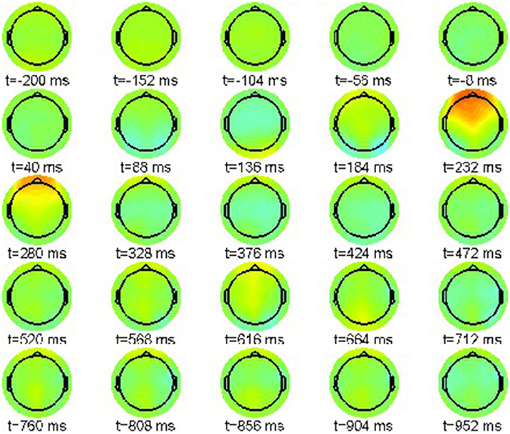
Figure 1. Snapshot sequence of ERP scalp topographies for correct condition (22-a).

The sequence exhibits only one prominent pattern, a frontal positivity around 232 ms, known as the attentional P200 component.

Accordingly, we present in Figure 2 the grand average for the phrase structure violation condition (22-b). Again the color scale ranges between [−15, 15]μV.

FIGURE 2

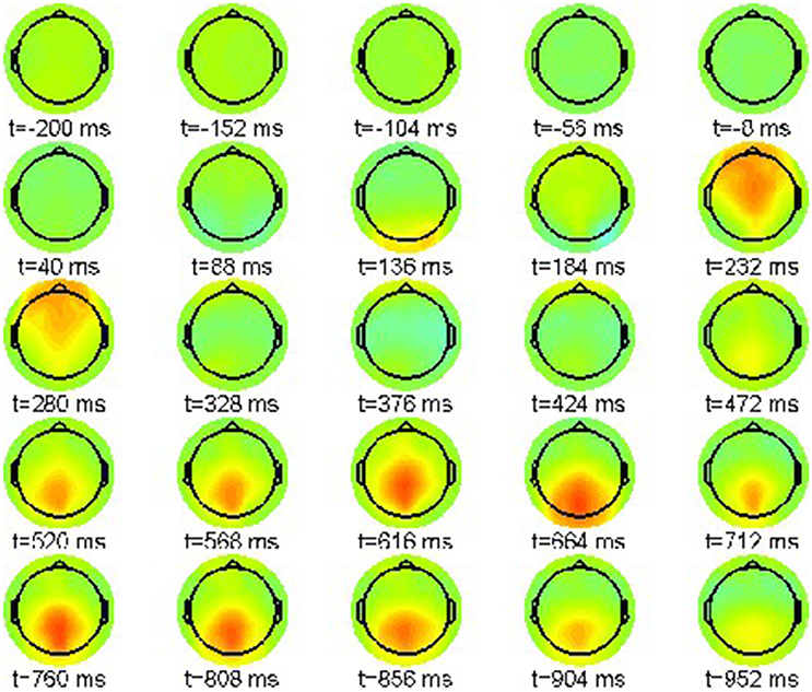
Figure 2. Snapshot sequence of ERP scalp topographies for violation condition (22-b).

Also in this condition the P200 effect is visible as a frontally pronounced positivity between 232 and 280 ms. Moreover, an earlier effect with reversed polarity can be recognized around 136 ms, the tentative N100 component. Most important is a parietal positivity starting at 472 ms until the end of the epoch window at 952 ms. This late positivity is commonly regarded as a neurophysiological correlate of syntactic violations [46], reanalysis [47, 48], ambiguity [49] and general integration problems [50].

However, a proper interpretation of ERP effects relies on considering condition differences. Thus, we plot the ERP difference between violation condition (22-b) and correct condition (22-a) in the range [−8, 8]μV in Figure 3.

FIGURE 3

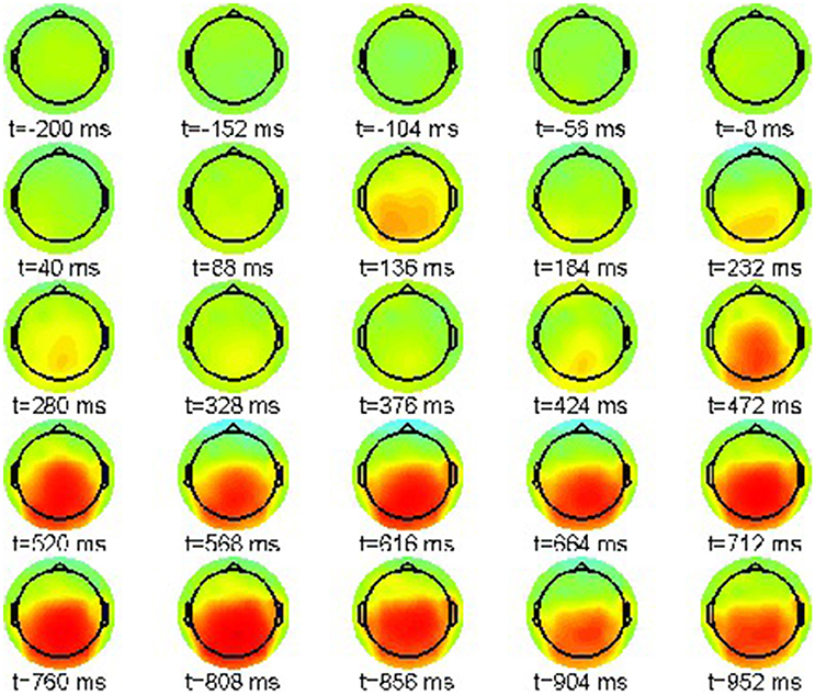
Figure 3. Snapshot sequence of ERP scalp topographies for difference potential, cf. movie data.gif in Supplementary Material.

The difference patterns in Figure 3 clearly indicate the posteriorly distributed P600 ERP component that evolves between 500 and 1,000 ms post-stimulus.

During cognitive tasks, Lehmann et al. [51, 53] and Wackermann et al. [52] observed segments of quasistationary EEG topographies, which they called brain microstates. The microstate analysis extracts MS in multivariate EEG signals based on the similarity of their spatial scalp distributions. It considers the multivariate EEG as a temporal sequence of spatial activity maps and extracts the time windows of the microstates by computing the temporal difference between successive maps. This procedure allows to compute the time windows of microstates from the signal and classifies them by the spatial averages over EEG electrodes in the extracted state time window.

In order to detect brain microstates by means of the RSA method in Section 2.1 we compute recurrence plots based on the cosine distance function

$\begin{array}{cc}{d}_{\cos }(x,y)=\frac{x·y}{\left|\right|x\left|\right|\left|\right|y\left|\right|}& \left(23\right)\end{array}$

as we are interested in detecting recurrent scalp topographies. This choice has also the advantage that the sparse 59-dimensional observation space is projected onto the unit sphere, resulting into a denser representation of ERP trajectories.

3. Results

Next we present the results of our ERP recurrence structure analysis and neural field modeling.

3.1. Recurrence Structure Analysis

For the recurrence structure analysis we optimize the Markov utility function (3) for the grand averages of both conditions (22-a) and (22-b) separately. The resulting utility functions are depicted in Figure 4.

FIGURE 4

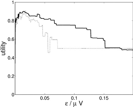
Figure 4. RSA Markov utility functions for conditions (22-a) (solid) and (22-b) (dotted).

Figure 4 indicates that both conditions lead to optimal segmentations for ε* ≈ 0.014.

The results of the recurrence structure analysis (RSA) for this optimal value of ε are shown in Figure 5. Figure 5A displays the grand average ERPs for the correct condition (22-a) and Figure 5B for the violation condition (22-b) where each colored trace denotes one recording electrode. The language-related P600 ERP component is clearly visible in Figure 5B as a positive going half-wave across many recording sites. The resulting segmentations are shown in Figure 5C for condition (22-a) and Figure 5D for condition (22-b) after additional Hausdorff clustering (θ = 0.25) for alignment between conditions. Moreover, we present the centers of gravity Equation (10) in Figure 5E for condition (22-a) and Figure 5F for condition (22-b) of the corresponding segments. The ERPs of both conditions start in a metastable baseline state 1 in the pre-stimulus interval. After a first transient (dark blue) still in the pre-stimulus interval both ERPs proceed into another baseline state 2. The P200 attentional component is realized as segment 3 in both conditions. Yet in condition (22-b) also the earlier N100 is detectable as MS 7 that does not exist in condition (22-a). The remaining segments 4, 5, 6 in the control condition (22-a) exhibit rather spatially flat topographies (cf. Figure 5E,F). While MS 6 is common to both conditions, the final state 8 in condition (22-b) reflects the crucial difference, namely the posteriorly distributed positive P600 component. These results are in full agreement with the understanding of language processing.

FIGURE 5

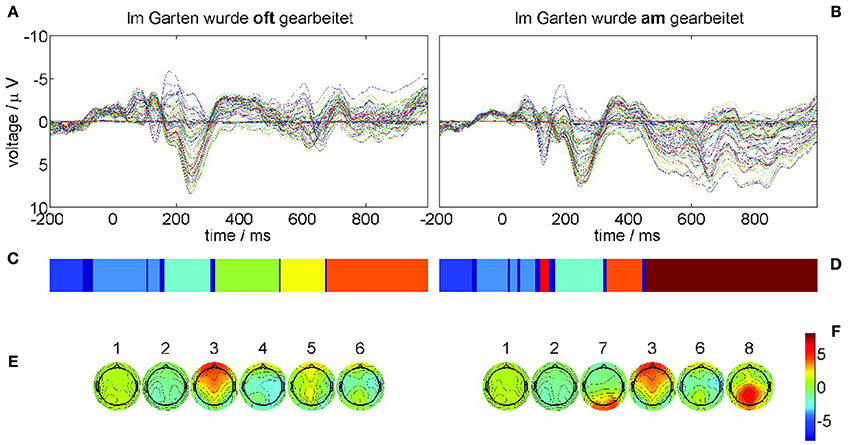
Figure 5. ERP grand averages and optimal recurrence grammar partition for experimental data taken from [44]. The panels (A,C,E) show results for the correct condition (22-a), the panels (B,D,F) for the phrase structure violation condition (22-b). (A,B) grand average ERPs over 17 subjects for all EEG channels, e.g., blue = electrode C5, green = electrode T7, and red = electrode FC5 (according to the 10–20 system of EEG electrode placement); each trace shows the time series of measured voltages in one recording channel. (C,D) Optimal encodings p aligned through Hausdorff clustering, where each color denotes one symbol. (E,F) Centers of gravity as time-averaged scalp topographies. The numbers denote the segment numbers. The P600 ERP component corresponds to segment 8. It is important to note that the voltage axis is inverted according to the EEG literature.

3.2. Neural Field Construction

After identification of the MS, we construct the neural field model based on results of Section 2.2. First we present the functional connectivity kernels w^(c)(x, y) for conditions (22-a) (c = 1) and (22-b) (c = 2) in Figures 6A,B. Figure 6C additionally displays the kernel difference w⁽²⁾(x, y) − w⁽¹⁾(x, y). For better visualization, we have ordered the recording electrodes according to their hemispheric topography, thus creating nine “regions of interest” (ROI): LF: left-frontal, LT: left-temporal, LP: left-parietal, LO: left-occipital, C: central (midline electrodes), RF: right-frontal, RT: right-temporal, RP: right-parietal, RO: right-occipital².

FIGURE 6

Figure 6. Reconstructed connectivity kernels for the neural field models for conditions (22-a) (A) and (22-b) (B); the difference kernel is shown in (C). Recording channels are given in topographic order: LF, left-frontal; LT, left-temporal; LP, left-parietal; LO, left-occipital; C, central (midline electrodes); RF, right-frontal; RT, right-temporal; RP, right-parietal; RO, right-occipital.

Figure 6 reveals a kind of checkerboard texture for the kernels w^(c)(x, y). Mostly obvious is the strength along the main diagonal, indicating mainly self-connections within brain areas, such as in ROIs LO and RO. Since primary visual cortex V1 is situated at occipital brain areas, these patterns may be interpreted as reflecting the visual presentation paradigm of the experiment. Interestingly, also the kernel difference exhibits largest differences in LO-LO and RO-RO areas. There is also a hemispheric asymmetry between reciprocal connections of left-parietal (LP) with left-occipital (LO) and right-parietal (RP) with right-occipital (RO) areas. It is quite tempting to speculate that this asymmetry is due to the brain's asymmetry regarding language processing: The largest difference between conditions is in the RF area, which is strong for the correct condition (22-a), but rather weak for the phrase structure violation condition (22-b). This might be seen as a neural correlate of semantic and pragmatic integration processes that are supported by the right hemisphere [50]. These processes fail in the case of the violation condition.

Next we show the simulated spatiotemporal dynamics of the neural field simulation from Section 2.2. To this end, the dynamics is illustrated as a temporal snapshot sequence of spatial topographies.

Figure 7 shows the simulation results for the correct condition (22-a) where every snapshot presents the neural field activation pattern at the indicated point in time. The color scale range is [−10, 10]μV.

FIGURE 7

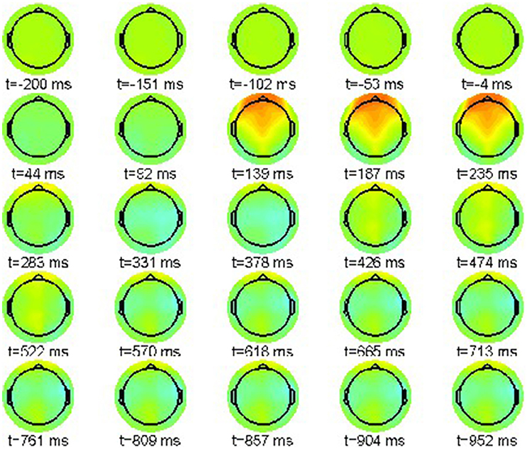
Figure 7. Snapshot sequence of neural field scalp topographies for correct condition (22-a).

The sequence exhibits one prominent pattern, a frontal positivity around 235 ms, reflecting the attentional P200 component. Hence it resembles well the original time series shown in Figure 1.

Accordingly, we present in Figure 8 the simulated neural field for the phrase structure violation condition (22-b). Again the color scale ranges between [−10, 10]μV.

FIGURE 8

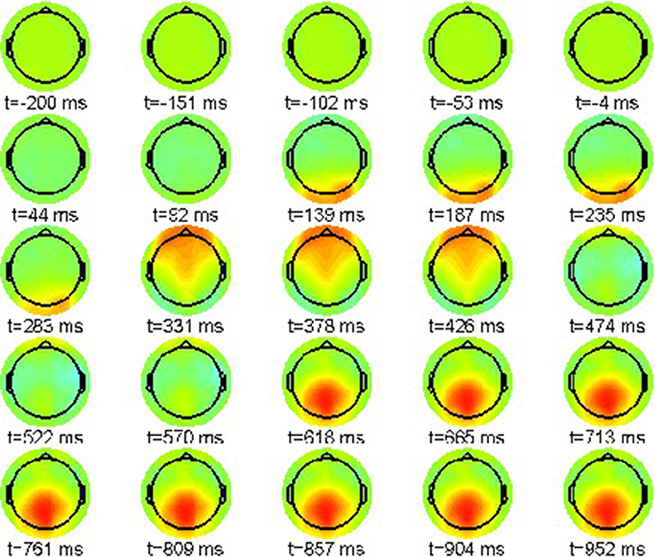
Figure 8. Snapshot sequence of neural field scalp topographies for violation condition (22-b).

In this condition the P200 effect is visible as a frontally pronounced positivity between 331 and 426 ms, however that is delayed compared to the original ERP data (cf. Figure 2). Hence our simulation entails a desynchronization in comparison with the experimentally observed ERP dynamics. The reason for this deviation is the presence of only one time scale in the underlying dynamic model, reflected by the growth rates of neural populations in the Lotka-Volterra Equation (14) that are all of the same order of magnitude. Hence, the phasic MS 7 is not appropriately captured by our phenomenological model.

Moreover, the earlier N100 component with reversed polarity is now shifted toward the time window between 139 and 235 ms. The final parietal positivity starting off at about 470 ms in the ERP data is already present in our simulation, now starting at 618 ms until the end of the epoch window at 952 ms.

As above, a proper interpretation of ERP effect requires the computation of condition differences. We plot the simulated neural field difference between violation condition (22-b) and correct condition (22-a) in the range [−10, 10]μV in Figure 9 similar to the ERP difference plot shown in Figure 3.

FIGURE 9

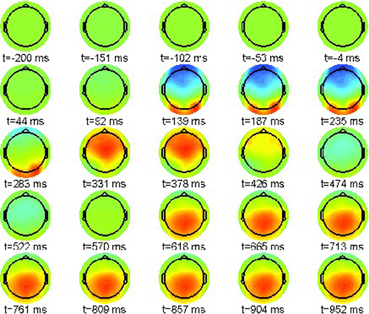
Figure 9. Snapshot sequence of neural field scalp topographies for difference potential, cf. movie model.gif in Supplementary Material.

A strong artifact effect from 139 until 235 ms is visible that is due to the misalignment of N100 and P200 in both conditions. However, the difference patterns clearly indicate the posteriorly distributed P600 ERP component that evolves between 618 and 1,000 ms post-stimulus.

3.3. RSA Validation

For the recurrence structure analysis of the neural field simulation we optimize the Markov utility function (3) for the grand averages of both conditions (22-a) and (22-b) separately. The resulting utility functions are depicted in Figure 10.

FIGURE 10

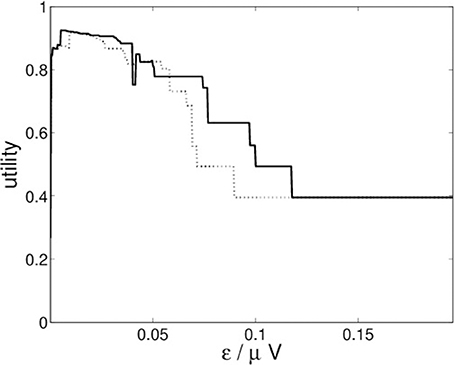
Figure 10. RSA Markov utility functions for neural fields simulations for conditions (22-a) (solid) and (22-b) (dotted).

Figure 10 indicates that both conditions lead to optimal segmentations for ε* ≈ 0.0051.

The results of the recurrence structure analysis (RSA) are shown in Figure 11.

FIGURE 11

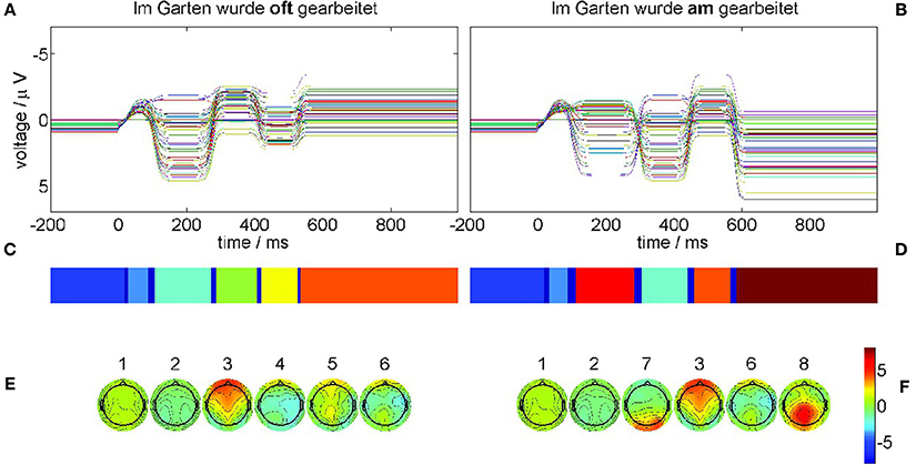
Figure 11. Neural field simulation and its optimal recurrence grammar partition for experimental data from Frisch et al. [44]. The panels (A,C,E) show results for the correct condition (22-a), the panels (B,D,F) for the phrase structure violation condition (22-b). (A,B) The time series of the simulated EEG channels in the respective condition. (C,D) Optimal encodings p aligned through Hausdorff clustering. (E,F) Centers of gravity as time-averaged spatial scalp topographies. The P600 ERP component corresponds to segment 8.

Figure 11A displays the simulated neural fields for the correct condition (22-a) and Figure 11B for the violation condition (22-b) where each colored trace denotes one simulated electrode. In both simulations the initial conditions were prepared as the stationary base line state 1 that does not change during the pre-stimulus interval. At stimulation time t = 0 a slight perturbation kicks the state out of equilibrium, triggering the sequential heteroclinic dynamics. The resulting segmentations are shown in Figure 11C for condition (22-a) and Figure 11D for condition (22-b) after additional Hausdorff clustering (θ = 0.1) for alignment between conditions. Despite the timing differences the pattern sequence is essentially the same as in Figure 5. This is confirmed by the centers of gravity Equation (10) in Figure 11E for condition (22-a) and Figure 11F for condition (22-b) of the corresponding segments. The simulated ERPs of both conditions start in a metastable baseline state 1 in the pre-stimulus interval. After a first transient (dark blue) still in the pre-stimulus interval both ERPs proceed into another baseline state 2. The P200 attentional component is realized as segment 3 in both conditions. In condition (22-b) also the earlier N100 is detectable as MS 7 yet with much longer duration than in the experimental ERP analysis. The remaining segments 4, 5, 6 in the control condition (22-a) exhibit rather flat topographies. While MS 6 is common to both conditions, the final state 8 in condition (22-b) reflects the crucial difference, namely the posteriorly distributed positive P600 component.

4. Discussion

The present work illustrates how to extract MS in a HO in experimental time series and how to model the sequence of metastable attractors. Both the feature extraction and the modeling part is based on underlying model assumptions on the dynamics of the heteroclinic sequence. The RSA is based on a stochastic Markov chain model, while the HO model is supposed to obey a Lotka-Volterra dynamics that can be mapped to a heterogeneous neural field equation.

The application to measured EEG data demonstrates that the combination of the feature extraction and modeling part allows to describe the heteroclinic sequences of metastable attractors in good agreement to experimental data. It is possible to reproduce the sequence of states and the time-averaged mean of the states well. However, details of the heteroclinic sequence, such as variability of durations of states and the duration of transients, may not be captured by both the feature extraction and/or the HO model and may stipulate closer investigations. This is seen in the simulated EEG data of Figure 8 that shows such differences to the experimental data.

The methodology presented improves previous attempts to derive dynamical models of HO in experimental brain data by the combination of RSA and the HO model for neural fields. The work introduces a novel approach based on Hausdorff clustering to combine several symbolic sequences gained from different experimental conditions to distinguish common and distinct MS. This analysis provides insights at which time instant and for which spatial EEG distribution common underlying mechanisms are present and when the brain behaves characteristically in different conditions. Moreover, the analysis provides spatial kernels of the neural field models for each experimental condition. The spatial kernels exhibit a hemispheric asymmetry reflecting the brains asymmetry in language processing, e.g., the semantic and pragmatic integration processes supported by the right hemisphere.

Models of heteroclinic sequences exhibit sequences of metastable attractors including attractive and repelling manifolds. By virtue of this construction, the dynamics is sensitive to random fluctuations yielding uncontrolled jumps outside the basin of attraction of the heteroclinic cycle and the divergence from the stationary cycle. The probability to leave the basin of attraction is small for tiny noise levels while increasing the noise level endangers the system to diverge. However, we point out that the modeled stable heteroclinic sequence is constructed in such a way that it is rather stable toward small levels of noise due to the dissipation [6]. This sensitivity may limit the applicability of the model proposed and requests either less noise-sensitive models [54] or noise-induced heteroclinic orbits [55].

Future work will apply the Hausdorff clustering to additional intracranially measured Local Field Potentials in animals and human EEG recordings to explore gain deeper insights into the brains heteroclinic underlying dynamics. For the neural field simulation, HO with multiple time scales as discussed by Yildiz and Kiebel [14] and beim Graben and Hutt [36] may be suitable to avoid alignment artifacts between MS.

Ethics Statement

The data has been taken from a study published previously in Frisch et al. [44].

Author Contributions

AH conceived the structure of the manuscript, PB performed the simulations and data analysis and both authors have written the manuscript.

Conflict of Interest Statement

The authors declare that the research was conducted in the absence of any commercial or financial relationships that could be construed as a potential conflict of interest.

Supplementary Material

The Supplementary Material for this article can be found online at: https://www.frontiersin.org/article/10.3389/fams.2017.00011/full#supplementary-material

Footnotes

1. ^Note that this recoding scheme applies accordingly to the case of more than two conditions.

2. ^Electrode selection for ROIs: left-frontal (LF) = “FP1,” “AF3,” “AF7,” “F9,” “F7,” “F5,” “F3,” “FC5,” “FC3”; left-temporal (LT) = “FT9,” “FT7,” “T7,” “C5,” “C3,” “TP9,” “TP7,” “CP5,” “CP3,” left-parietal (LP) = “P9,” “P7,” “P5,” “P3”; left-occipital (LO) = “O1,” “PO7,” “PO3”; midline-central (C) = “FPZ,” “AFZ,” “FZ,” “FCZ,” “CZ,” “CPZ,” “PZ,” “POZ,” “OZ”; right-frontal (RF) = “FP2,” “AF4,” “AF8,” “F10,” “F8,” “F6,” “F4,” “FC6,” “FC4”; right-temporal (RT) = “FT10,” “FT8,” “T8,” “C6,” “C4,” “TP10,” “TP8,” “CP6,” “CP4”; right-parietal (RP) = “P10,” “P8,” “P6,” “P4”; right-occipital (RO) = “O2,” “PO8,” “PO4.”

References

1. Tsuda I. Toward an interpretation of dynamic neural activity in terms of chaotic dynamical systems. Behav Brain Sci. (2001) 24:793–810. doi: 10.1017/S0140525X01000097

PubMed Abstract | CrossRef Full Text | Google Scholar

2. Guckenheimer J, Holmes P. Nonlinear oscillations, dynamical systems, and bifurcations of vector fields. In: Applied Mathematical Sciences, Vol. 42. New York, NY: Springer (1983).

3. Afraimovich VS, Zhigulin VP, Rabinovich MI. On the origin of reproducible sequential activity in neural circuits. Chaos (2004) 14:1123–9. doi: 10.1063/1.1819625

PubMed Abstract | CrossRef Full Text | Google Scholar

4. Rabinovich MI, Huerta R, Varona P, Afraimovich VS. Transient cognitive dynamics, metastability, and decision making. PLoS Comput Biol. (2008) 4:e1000072. doi: 10.1371/journal.pcbi.1000072

PubMed Abstract | CrossRef Full Text | Google Scholar

5. Ashwin P, Postlethwaite C. On designing heteroclinic networks from graphs. Physica D (2013) 265:26–39. doi: 10.1016/j.physd.2013.09.006

CrossRef Full Text | Google Scholar

6. Afraimovich VS, Moses G, Young T. Two-dimensional heteroclinic attractor in the generalized Lotka-Volterra system. Nonlinearity (2016) 29:1645. doi: 10.1088/0951-7715/29/5/1645

CrossRef Full Text | Google Scholar

7. Busse FH Heikes KE. Convection in a rotating layer: a simple case of turbulence. Science (1980) 208:173–5. doi: 10.1126/science.208.4440.173

PubMed Abstract | CrossRef Full Text | Google Scholar

8. Hutt A, Svensén M, Kruggel F, Friedrich R. Detection of fixed points in spatiotemporal signals by a clustering method. Phys Rev E (2000) 61:R4691–3. doi: 10.1103/PhysRevE.61.R4691

PubMed Abstract | CrossRef Full Text | Google Scholar

9. Lorenz EN. Deterministic nonperiodic flow. J Atmospher. Sci. (1963) 20:130–141.

Google Scholar

10. Fingelkurts AA, Fingelkurts AA. Making complexity simpler: multivariability and metastability in the brain. Int J Neurosci. (2004) 114:843–62. doi: 10.1080/00207450490450046

PubMed Abstract | CrossRef Full Text | Google Scholar

11. Fingelkurts AA, Fingelkurts AA. Information flow in the brain: ordered sequences of metastable states. Information (2017) 8:22. doi: 10.3390/info8010022

CrossRef Full Text | Google Scholar

12. beim Graben P, Hutt A. Detecting event-related recurrences by symbolic analysis: applications to human language processing. Philos Trans R Soc Lond. (2015) A373:20140089. doi: 10.1098/rsta.2014.0089

CrossRef Full Text | Google Scholar

13. Mazor O, Laurent G. Transient dynamics versus fixed points in odor representations by locust antennal lobe projection neurons. Neuron (2005) 48:661–73. doi: 10.1016/j.neuron.2005.09.032

PubMed Abstract | CrossRef Full Text | Google Scholar

14. Yildiz IB, Kiebel SJ. A hierarchical neuronal model for generation and online recognition of birdsongs. PLoS Comput Biol. (2011) 7:e1002303. doi: 10.1371/journal.pcbi.1002303

PubMed Abstract | CrossRef Full Text | Google Scholar

15. Ville DD, Britz J, Michel CM. EEG microstate sequences in healthy humans at rest reveal scale-free dynamics. Proc Natl Acad Sci USA (2010) 107:18179–84. doi: 10.1073/pnas.1007841107

PubMed Abstract | CrossRef Full Text | Google Scholar

16. Musso F, Brinkmeyer J, Mobascher A, Warbrick T, Winterer G. Spontaneous brain activity and EEG microstates. A novel EEG/fMRI analysis approach to explore resting-state networks. NeuroImage (2010) 52:1149–61. doi: 10.1016/j.neuroimage.2010.01.093

PubMed Abstract | CrossRef Full Text | Google Scholar

17. Uhl C, Kruggel F, Opitz B, von Cramon DY. A new concept for EEG/MEG signal analysis: detection of interacting spatial modes. Hum Brain Mapp. (1998) 6:137–149.

PubMed Abstract | Google Scholar

18. Tomescu MI, Rihs TA, Becker R, Britz J, Custo A, Grouiller F, et al. Deviant dynamics of EEG resting state pattern in 22q11.2 deletion syndrome adolescents: a vulnerability marker of schizophrenia?, Schizophr Res. (2014) 157:175–81. doi: 10.1016/j.schres.2014.05.036

PubMed Abstract | CrossRef Full Text | Google Scholar

19. Hudson AE, Calderon DP, Pfaff DW, Proekt A. Recovery of consciousness is mediated by a network of discrete metastable activity states. Proc Natl Acad Sci USA (2014) 111:9283–8. doi: 10.1073/pnas.1408296111

PubMed Abstract | CrossRef Full Text | Google Scholar

20. Ito J, Nikolaev AR, van Leeuwen C. Dynamics of spontaneous transitions between global brain states. Hum Brain Mapp. (2007) 28:904–13. doi: 10.1002/hbm.20316

PubMed Abstract | CrossRef Full Text | Google Scholar

21. Bersini H, Sener P. The connections between the frustrated chaos and the intermittency chaos in small Hopfield networks. Neural Netw. (2002) 15:1197–204. doi: 10.1016/S0893-6080(02)00096-5

PubMed Abstract | CrossRef Full Text | Google Scholar

22. Hutt A, and Riedel H. Analysis and modeling of quasi-stationary multivariate time series and their application to middle latency auditory evoked potentials. Physica D (2003) 177:203–32. doi: 10.1016/S0167-2789(02)00747-9

CrossRef Full Text | Google Scholar

23. Haken H, editor. Synergetics. An introduction. In: Springer Series in Synergetics, 3rd Edn., 1st Edn., 1977, vol. 1. Berlin: Springer (1983).

24. Haken H, editor. Principles of brain functioning. In: Springer Series in Synergetics, vol. 67. Berlin: Springer (1996).

25. Hutt A. An analytical framework for modeling evoked and event-related potentials. Int J Bifurcat Chaos (2004) 14:653–66. doi: 10.1142/S0218127404009351

CrossRef Full Text | Google Scholar

26. beim Graben P, Hutt A. Detecting recurrence domains of dynamical systems by symbolic dynamics. Phys Rev Lett. (2013) 110:154101. doi: 10.1103/PhysRevLett.110.154101

CrossRef Full Text | Google Scholar

27. beim Graben P, Sellers KK, Fröhlich F, Hutt A. Optimal estimation of recurrence structures from time series. EPL (2016) 114:38003. doi: 10.1209/0295-5075/114/38003

CrossRef Full Text | Google Scholar

28. Takens F. Detecting strange attractors in turbulence. In Rand DA, Young LS, editors. Dynamical Systems and Turbulence, volume 898 of Lecture Notes in Mathematics. Berlin: Springer (1981). p. 366–81.

Google Scholar

29. Fedotenkova M, beim Graben P, Sleigh J, Hutt A. Time-frequency representations as phase space reconstruction in recurrence symbolic analysis. In: International Work-Conference on Time Series (ITISE), Granada. (2016).

Google Scholar

30. Tošić T, Sellers KK, Fröhlich F, Fedotenkova M, beim Graben P, Hutt A. Statistical frequency-dependent analysis of trial-to-trial variability in single time series by recurrence plots. Front Syst Neurosci. (2016) 9:184.

PubMed Abstract | Google Scholar

31. Poincaré H. Sur le problème des trois corps et les équations de la dynamique. Acta Math. (1890) 13:1–270.

Google Scholar

32. Eckmann JP, Kamphorst SO, Ruelle D. Recurrence plots of dynamical systems. Europhys Lett. (1987) 4:973–977. doi: 10.1209/0295-5075/4/9/004

CrossRef Full Text | Google Scholar

33. Marwan N, Kurths J. Line structures in recurrence plots. Phys Lett. (2005) 336:349–57. doi: 10.1016/j.physleta.2004.12.056

CrossRef Full Text

34. Rote G. Computing the minimum Hausdorff distance between two point sets on a line under translation. Inform Process Lett. (1991) 38:123–7. doi: 10.1016/0020-0190(91)90233-8

CrossRef Full Text | Google Scholar

35. Coombes S, beim Graben P, Potthast. Tutorial on neural field theory. In: Coombes S, beim Graben P, Potthast R, Wright J, editors. Neural Fields: Theory and Applications. Berlin: Springer (2014). p. 1–43.

Google Scholar

36. beim Graben P, Hutt A. Attractor and saddle node dynamics in heterogeneous neural fields. EPJ Nonlin Biomed Phys. (2014) 2:4. doi: 10.1140/epjnbp17

CrossRef Full Text | Google Scholar

37. Hutt A, Hashemi M, beim Graben P. How to render neural fields more realistic. In: Bhattacharya BS, Chowdhury FN, editors. Validating Neuro-Computational Models of Neurological and Psychiatric Disorders, Springer Series in Computational Neuroscience. Berlin: Springer (2015). p. 141–59.

Google Scholar

38. Schwappach C, Hutt A, beim Graben P. Metastable dynamics in heterogeneous neural fields. Front Syst Neurosci. (2015) 9:97. doi: 10.3389/fnsys.2015.00097

PubMed Abstract | CrossRef Full Text | Google Scholar

39. Amari SI. Dynamics of pattern formation in lateral-inhibition type neural fields. Biol Cybern. (1977) 27:77–87. doi: 10.1007/BF00337259

PubMed Abstract | CrossRef Full Text | Google Scholar

40. beim Graben P, Potthast R. A dynamic field account to language-related brain potentials. In: Rabinovich M, Friston K, Varona P, editors. Principles of Brain Dynamics: Global State Interactions. Cambridge, MA: MIT Press (2012). p. 93–112.

Google Scholar

41. Veltz R, Faugeras O. Local/global analysis of the stationary solutions of some neural field equations. SIAM J Appl Dyn Syst. (2010) 9:954–98. doi: 10.1137/090773611

CrossRef Full Text | Google Scholar

42. Hertz J, Krogh A, Palmer RG. Introduction to the theory of neural computation. In: Lecture Notes of the Santa Fe Institute Studies in the Science of Complexity, vol. I. Cambridge, MA: Perseus Books (1991).

43. beim Graben P, Potthast R. Inverse problems in dynamic cognitive modeling. Chaos (2009) 19:015103. doi: 10.1063/1.3097067

CrossRef Full Text | Google Scholar

44. Frisch S, Hahne A, Friederici AD. Word category and verb-argument structure information in the dynamics of parsing. Cognition (2004) 91:191–219. doi: 10.1016/j.cognition.2003.09.009

PubMed Abstract | CrossRef Full Text | Google Scholar

45. Birkhoff G, von Neumann J. The logic of quantum mechanics. Ann Math. (1936) 37:823–843. doi: 10.2307/1968621

CrossRef Full Text | Google Scholar

46. Osterhout L, Holcomb PJ. Event-related brain potentials elicited by syntactic anomaly. J Mem Lang. (1992) 31:785–806. doi: 10.1016/0749-596X(92)90039-Z

CrossRef Full Text | Google Scholar

47. Osterhout L, Holcomb PJ, Swinney DA. Brain potentials elicited by garden-path sentences: evidence of the application of verb information during parsing. J Exp Psychol Learn Mem Cogn. (1994) 20:786–803. doi: 10.1037/0278-7393.20.4.786

PubMed Abstract | CrossRef Full Text | Google Scholar

48. beim Graben P, Saddy D, Schlesewsky M, Kurths J. Symbolic dynamics of event-related brain potentials. Phys Rev E (2000) 62:5518–41. doi: 10.1103/PhysRevE.62.5518

CrossRef Full Text | Google Scholar

49. Frisch S, Schlesewsky M, Saddy D, Alpermann A. The P600 as an indicator of syntactic ambiguity. Cognition (2002) 85:B83–92. doi: 10.1016/S0010-0277(02)00126-9

PubMed Abstract | CrossRef Full Text | Google Scholar

50. Brouwer H, Fitz H, Hoeks J. Getting real about Semantic Illusions: rethinking the functional role of the P600 in language comprehension. Brain Res. (2012) 1446:127–43. doi: 10.1016/j.brainres.2012.01.055

PubMed Abstract | CrossRef Full Text | Google Scholar

51. Lehmann D, Ozaki H, Pal I. EEG alpha map series: brain micro-states by space-oriented adaptive segmentation. Electroencephalogr Clin Neurophysiol. (1987) 67:271–88. doi: 10.1016/0013-4694(87)90025-3

PubMed Abstract | CrossRef Full Text | Google Scholar

52. Wackermann J, Lehmann D, Michel CM, Strik WK. Adaptive segmentation of spontaneous EEG map series into spatially defined microstates. Int J Psychophysiol. (1993) 14:269–83. doi: 10.1016/0167-8760(93)90041-M

PubMed Abstract | CrossRef Full Text | Google Scholar

53. Lehmann D, Pascual-Marqui RD, Michel C. EEG microstates. Scholarpedia (2009) 4:7632. doi: 10.4249/scholarpedia.7632

CrossRef Full Text | Google Scholar

54. Gasner S, Blomgren P, Palacios A. Noise-induced intermittency in cellular pattern-forming systems. Int J Bifurcation Chaos (2007) 17:2765. doi: 10.1142/S0218127407018749

CrossRef Full Text | Google Scholar

55. Armbruster D, Stone E, Kirk V. Noisy heteroclinic networks. Chaos (2003) 13:71–79. doi: 10.1063/1.1539951

CrossRef Full Text | Google Scholar