Specifying Turning Point in Piecewise Growth Curve Models: Challenges and Solutions

Introduction

Longitudinal studies have been widely applied in many research areas to examine individual differences in growth over time. One commonly used method to study individual change over time is the latent growth modeling in the Structural Equation Modeling (SEM) framework [1, 2]. Up to date, the majority of applications of the latent growth models in longitudinal data analyses have been limited to the assumption that the change follows a simple linear trend. However, when longitudinal data are collected over an adequately long period of time, the features of individual change do not always follow a linear trend.

A more flexible approach to model the nonlinear form of growth is the piecewise growth curve model (PGCM). This approach breaks up the curvilinear growth trend into separate linear segments or pieces of different slopes, which are tied together by turning points (or knots or change points). The flexibility of PGCM allows the formulation of different functional forms for the different phases of growth such that each phase does not have to conform to the same function [3–6]. The approach is particularly appealing when researchers are interested in comparing growth rates for two or more periods, such as the effect of schooling on children's scholastic attainments before and after secondary school [7, 8].

The major difficulty in applying PGCMs concerns the specification of the turning point. Researchers tend to rely on theories or designs (e.g., the start point of an intervention) to choose the location of the turning point (see e.g., [9, 10]). Yet, such considerations may not always be reasonable. For example, the turning point may occur after the intervention due to delay in response to intervention. The misspecification of a turning point may render a suboptimal functional representation of the observed data patterns, leading to incorrect inferences of growth traits.

Alternative approaches were developed to search for the optimal location of the turning point based on data [6, 11, 12]. For example, Kwok et al. [6] proposed using modification index to detect the turning point in the linear latent growth modeling framework. Harring et al. [3] extended PGCM to treat the turning point as an unknown parameter to be estimated in the SEM framework. Compared to the conventional PGCM with turning points specified a priori, such an extension is appealing because researchers do not have to have a priori knowledge of the turning points. Moreover, allowing for free estimation of turning points and time specific factor loadings can lead to a more optimal functional form of each growth phase, giving a more adequate description of the growth pattern in the data [6, 13]. The appealing advantages of the newly proposed PGCM with unknown turning points have attracted an increasing amount of interest in empirical studies (see e.g., [5, 14, 15]).

Comparing and contrasting the conventional and the new PGCM, this study aims to investigate the three research questions. First, under what conditions and to what extent does the misspecification of turning point in conventional PGCMs have a substantial impact on the growth trait estimation? Second, in conventional PGCMs, can the commonly used fit indices correctly identify model misspecification due to the mislocation of turning points? Lastly, can the new procedure of PGCM with an unknown turning point accurately estimate the turning point and growth parameters?

The remaining of the paper is organized in the following sections. We first reviewed the model specification for the new PGCM with an unknown turning point, followed by a brief description of commonly used fit indexes under the SEM framework. Then we introduced the methods for data generation, analysis procedure, and presented the findings from the simulation study. Finally, we discussed the findings in relation to previous studies, implications, and limitations.

PGCM with One Unknown Turning Point

Suppose that the sample data consist of j equal spaced repeated measures of Y for individual i. A two-piece growth model with one unknown turning point can be specified in the form of two-level models. The Level 1 (repeated measures) model is specified as

$\begin{array}{ll}{\text{y}}_{ij}=\{\begin{array}{c}{\text{l}}_1(\text{t}):{\text{a}}_{1\text{i}}+{\text{b}}_{1\text{i}}({\text{t}}_{\text{ij}})+{\epsilon }_{\text{ij}}{\text{t}}_{\text{ij}}⩽\gamma \\ {\text{l}}_2(\text{t}):{\text{a}}_{2\text{i}}+{\text{b}}_{2\text{i}}({\text{t}}_{\text{ij}})+{\epsilon }_{\text{ij}}{\text{t}}_{\text{ij}}>\gamma \end{array}& (1)\end{array}$

where y_ij is the response at the jth measurement for the ith individual. a_1i and b_1i are the intercept and the slope growth factors before the occurrence of the turning point, and a_2i and b_2i denote the corresponding growth factors after the turning point. γ is the location of the turning point marking the shift from one growth phase to the other. ε_ij is the level-1 residual for individual i at measurement j [${\epsilon }_{ij}~N(0,{\sigma }_{\epsilon }^2)$]. It is assumed that the location of the turning point is fixed to be the same for all individuals. Hence the model is appropriate when homogeneous turning points are assumed. For example, studies have found that almost all the average children have been able to establish their numerical and arithmetic foundation in 3rd grade, which could be assumed to be a common turning point in the development of child numerical cognition (see e.g., [16]).

The trajectory is assumed to be continuous and has no gap between the two pieces, such that the two pieces for l₁(t) and l₂(t) are connected at the turning point. That is, when t_ij = γ, a_1i + b_1i(γ) = a_2i + b_2i(γ), which gives a_2i = a_1i + γ(b_1i − b_2i). Thus Model (Equation 1) that has five parameters is reduced to a four-parameter model

$\begin{array}{l}{\text{y}}_{ij}=\{\begin{array}{c}{\text{l}}_1(\text{t}):{\text{a}}_{1\text{i}}+{\text{b}}_{1\text{i}}({\text{t}}_{\text{ij}})+{\epsilon }_{\text{ij}}{\text{t}}_{\text{ij}}⩽\gamma \hfill \\ {\text{l}}_2(\text{t}):{\text{a}}_{1\text{i}}+{\text{b}}_{1\text{i}}\gamma +{\text{b}}_{2\text{i}}(t_{\text{ij}}-\gamma )+{\epsilon }_{\text{ij}}{\text{t}}_{\text{ij}}>\gamma \hfill & (2)\end{array}\hfill \end{array}$

The Level-2 (between-subject) model is specified as

$\begin{array}{ll}\{\begin{array}{c}{\text{a}}_{1\text{i}}={\mu }_{a1}+{\zeta }_{a1\text{i}}\\ {\text{b}}_{1\text{i}}={\mu }_{b1}+{\zeta }_{b1\text{i}}\\ {\text{b}}_{2\text{i}}={\mu }_{b2}+{\zeta }_{b2\text{i}}\end{array}& (3)\end{array}$

with

$\begin{array}{ll}\left[\begin{array}{c}{\zeta }_{\text{a}1\text{i}}\\ {\zeta }_{\text{b}1\text{i}}\\ {\zeta }_{\text{b}2\text{i}}\end{array}\right]~\text{ MVN}\left(\left[\begin{array}{c}0\\ 0\\ 0\end{array}\right],\left[\begin{array}{ccc}{\tau }_{\pi 00}& {\tau }_{\pi 01}& {\tau }_{\pi 02}\\ {\tau }_{\pi 10}& {\tau }_{\pi 11}& {\tau }_{\pi 12}\\ {\tau }_{\pi 20}& {\tau }_{\pi 21}& {\tau }_{\pi 22}\end{array}\right]\right),& (4)\end{array}$

where μ_a1, μ_b1, and μ_b2 are growth factor means and ζ_a1, ζ_b1, and ζ_b2 are random disturbances in their respective growth factors. The Level 1 residuals and the Level 2 disturbances are also assumed to be uncorrelated with each other and with the latent growth factors.

The parameterization of Model (Equation 2) cannot be specified and estimated directly in conventional Structural Equation Modeling (SEM) programs. Harring et al. [3] suggested a re-parameterization of Model (Equation 2) to make the estimation in SEM programs possible. They proposed to combine the two linear trajectories in Model (Equation 2) into one equation ${\text{y}}_{\text{ij}}={\lambda }_{1\text{i}}+{\lambda }_{2\text{i}}{\text{t}}_{\text{ij}}+{\lambda }_{3\text{i}}\sqrt{{({\text{t}}_{\text{ij}}-\gamma )}^2}+{\epsilon }_{\text{ij}}$, where λ_1i = (a_1i + a_2i)/2, λ_2i = (b_1i + b_2i)/2, and λ_3i = (b_2i − b_1i)/2. Readers are referred to Harring et al. [3] and Kohli and Harring [5] for details of the model re-parameterization.

Sem-Based Fit Indices

The commonly used fit indices available in standard SEM software for applied researchers to determine the adequacy of their SEM models includes but not limited to root-mean-square error of approximation (RMSEA; [17]), standardized root-mean-square residual (SRMR; [18]), the Comparative Fit Index (CFI; [19]), and the Tucker-Lewis Index (TLI; [20]). Following the recommendation of Hu and Bentler [21, 22], the cutoff criteria for the commonly used fit indices (e.g., RMSEA ≤ 0.06; CFI ≥ 0.95; TLI ≥ 0.95; SRMR ≤ 0.08) have been generally used to assess model fit/misfit in SEM analysis. However, there has been controversy regarding the advocacy for the proposed fixed cutoff criteria. Applied researchers were warned against a complete reliance on fixed cutoff criteria in assessing model fit (see e.g., [23–25]). Simulation studies have been done in the context of confirmatory factor analysis (CFA) models, evaluating the performance of the fit indices in identifying misspecification in covariance structures (see e.g., [21, 23, 24]).

More relevant to the present research interest were the studies that addressed the sensitivity of fit indices in identifying misspecifications of growth shape. Wu et al. [26] derived theoretically that the SEM-based fit indices such as the Chi-Square, RMSEA, CFI and TLI were able to “directly detect” mis-specified functional form for the mean growth trajectory. Wu and West [27] evaluated the theoretical derivation using a simulation study to further understand the performance of the above mentioned fit indices in detecting model misspecification in covariance structures and marginal mean structure. In their study, the mean growth trajectory in the population model was quadratic GCM, but was mis-specified as linear GCM. Their findings with regards to the capabilities of fit indices in detecting mis-specified mean functional forms showed that RMSEA, CFI, and TLI were more sensitive to misspecification in marginal mean structure than Chi-square test statistic or SRMR, while the latter two were affected by sample size. Leite and Stapleton [28] found that comparatively speaking, the Chi-square test statistic performed the best, followed by RMSEA, relative to CFI, TLI, and SRMR in detecting model misfit in GCM, accounting for sample size, misspecification severity, number of time points, and population growth shapes, when the population data generated using quadratic, plateau, and piecewise GCMs were fitted using a (mis-specified) linear model. It is noteworthy that the baseline model used to calculate CFI and TLI for growth curve model is not appropriate in standard SEM software packages including the Mplus software. The appropriate baseline model is an intercept-only model in which only the intercept mean and residual variances are freely estimated [27, 29].

Another important piece of information that applied researchers tend to rely on for model fit improvement is modification index (MI) or Lagrange multiplier. What MI captures is an estimate of the expected change in the specified model's overall chi-square (χ²) value if a previously constrained parameter were allowed to be freely estimated. A large MI value suggests an appreciable improvement in model fit if the model were modified to freely estimate that particular parameter, given that the post hoc modification is theoretically justifiable. While MI provides the significance of the misspecification, EPC (expected parameter change) is an estimate of the impact of the misspecification on parameter estimates. EPC has been suggested to be used in conjunction with MI to detect model misspecification (see e.g., [30]). Several variations of EPC have been proposed: the unstandardized expected parameter change (EPC; [31]), which provides the estimated value that a given fixed parameter would have if it were freely estimated in the model; the partially standardized EPC [32], and the fully standardized EPC (SEPC; [33]), referred to as “Std YX E.P.C.” in the Mplus package (2007–2016). Interested readers are referred to Whittaker [34] for the differences between the variations of EPC.

Saris et al. [31] argued against the reliance on χ² test statistics and fit indices for model evaluation because they are not only affected by the degree of misspecification but also by the incidental characteristics of the model. Alternatively, they proposed to use MI along with EPCs. However, the decision on the presence of model misspecification can only be made when a large, significant MI is associated with a large EPC. Saris et al. [35] further suggested taking into account of the information on the power of the MI test when using the SEPC in combination with MI to make decision regarding model misspecification errors. They also suggested that a SEPC of 0.2 or larger is a large value, indicative of possible misspecification error. To evaluate whether a SEPC of 0.2 or larger can be implemented as a cutoff criterion of the SEPC in applied research, Whittaker [34] conducted a simulation study to examine the performance of the MI and SEPC in detecting misspecification errors when a correlated two-factor population model was mis-specified as an uncorrelated two-factor model. Her findings revealed that the SEPC cutoff criterion can identify misspecification 70% of the overall replications in 80% of all the manipulated conditions in her study and it performed more accurately than the MI even when sample sizes and factor loading sizes were both small. Overall, there have been no consistent findings regarding the accuracy and stability of MI and/or EPC in detecting model misspecification; some studies revealed promising performance of MI and/or EPC [6, 36], but a preponderance of research found the performance less than acceptable [30, 32, 37, 38].

In summary, the majority of previous research only investigated misspecification in covariance structure and the findings are inconsistent. Hence, it is necessary to evaluate the effectiveness of using fit indices, MIs, and SEPC to detect misspecifications on the growth shape due to mislocations of turning points.

Methods

Data Generation

A simulation study was conducted to address the above research questions. The population model used for data generation is a piece-to-piece linear growth model consisting of 7 equidistance time points and connected by one turning point. For simplicity, no covariates are included in the population model.

Based on the model defined by Equations (2–4), a total of 11 parameters are specified: four fixed effect coefficients (i.e., μ_a1, μ_b1, μ_b2, and γ) and seven variances and covariance of random effects (i.e., σ², τ_π00, τ_π10, τ_π20, τ_π11, τ_π21, τ_π22). Table 1 presents the population parameter values specified based on previous studies (see e.g., [39]).

TABLE 1

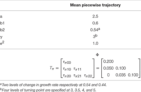
Table 1. Population parameters for the piecewise growth trajectory.

Design Factors

Based on previous findings regarding PGCM [5, 6, 27, 28], four design factors are considered, including (a) sample size, (b) the magnitude of change in the growth rate, (c) degree of severity in turning point misspecification, and (d) levels of non-normality.

Sample Size

The sample size was decided based on the empirical studies using piecewise latent growth curve modeling obtained from a literature search in PsycINFO (from 2010 to 2016). We chose three sample size conditions (75, 200, or 500 cases), representing approximately the minimum, 25th, and 50th percentiles of the sample size distribution.

Magnitude of Change in the Growth Rate

Based on Kwok et al.'s [6] study, we considered two levels in the magnitude change in growth rate: small change vs. medium change. Given that the growth rate in the first piece is 0.6, following Raudenbush and Liu's [39] effect size equation, the growth rate of the second piece is set to be 0.44 for the medium change condition and 0.54 for the small change condition.

Levels of Severity in Turning Point Misspecification

We generated data with four locations of turning point: 3, 3.5, 4, and 5 respectively. In the analysis model, the conventional PGCM specifies the turning point to be at time point 3. This is to mirror the two scenarios in reality: (1) the treatment began at time point 3, and was followed with an immediate change in growth rate (i.e., no misspecification); (2) the treatment effect was delayed (i.e., misspecification of 0.5, 1, or 2 time points).

Normality of Distributions

In longitudinal data, it is common to encounter non-normal data. To mimic real world data, we considered two conditions: normal and moderately skewed. For the moderately skewed distributions, the random effects were generated to have skewness of 1.5 and kurtosis of 6 respectively using Vale and Maurelli's [40] algorithm for simulating multivariate non-normal data. Such values are considered to be within the range of skewed distribution encountered in applied psychological research [41, 42].

In summary, the simulation used a 3 (number of sample size: 75 or 200 or 500) × 2 (magnitude of change in growth rate: small [B2 = 0.54] or medium [B2 =: 0.44]) × 4 (levels of severity of misspecification: 0, 0.5, 1, or 2 time points) × 2 (levels of distribution: normal or moderately skewed) factorial design to generate the data. A total of 500 replications were generated for each condition using SAS 9.4 Proc IML procedure [43], yielding 24,000 total data sets. Each replication was then fit with two different model specifications respectively: (1) the conventional PGCM with the turning point specified to be at the 3rd time point, and (2) the newly proposed PGCM with the turning point as an unknown parameter to be freely estimated. Both models were fit using Mplus version 7.4 [44] with Estimator = MLR. The Mplus code for the newly proposed PGCM is provided in the Appendix as a reference.

Analysis

Proper replications that reached convergence and had no improper solutions (e.g., negative variances) were retained for further analysis. The means and standard deviations of each fit index were presented along with their respective hit rates, which is a measure of the proportion of replications that successfully identified the correct or mis-specified models based on the recommended cutoff criteria (RMSEA ≤ 0.06; SRMR ≤ 0.08; TLI ≥ 0.95; FCI ≥ 0.95) recommended by Hu and Bentler [22].

For Modification Indexes (MI), because the purpose is to detect growth shape misspecification due to the incorrectly located turning point, we restricted the search of MIs among the loadings of time points 3 to 7 associated with the 1st piece and the 2nd piece growth factors. To maintain the family-wise Type I error at the 0.05 level, we adjusted the alpha level to be at 0.005 because there are a total number of 10 potential fixed loadings to be modified. Therefore, the threshold of a MI to be considered significant was 7.88 (df = 1 and α = 0.005). For SEPCs (the fully standardized Expected Parameter Changes), we used the cutoff value of 0.2 as recommended by Saris et al. [35].

Estimates of the turning point, growth parameters, their corresponding standard errors and the random effects were summarized across all proper replications for each condition. The standardized biases of the estimates [i.e., $B(\widehat{\theta })=(\widehat{\theta }-\theta )/S(\widehat{\theta })$]¹ were calculated. The mean of the standardized bias is equivalent to a Cohen's d, which measures the standardized distance between the estimate and the parameter. Based on the guidelines for Cohen's d, the value of less than 0.14 is considered acceptable. For turning point estimates, the unstandardized biases [i.e., $B(\widehat{\theta })=\widehat{\theta }-\theta$] were also calculated to show the bias in the original metric of time.

Analysis of variance (ANOVA) was then used to examine the impact of the design factors on the bias of the parameter estimates. The eta-squared (${\eta }^2=S{S}_{\text{Effect}}/S{S}_{\text{Total}}$) effect size was computed and reported as a measure of practical significance. Effects were considered substantial with the eta-squared greater than 0.1.

Results

Model convergence was explicitly examined to ensure a clear and appropriate analysis of the results. All 500 replications in each of the designed conditions, estimated using the conventional PGCM with the turning point determined a priori, converged successfully with no improper solutions. For the PGCM with an unknown turning point, the average convergence rate was around 80%. Non-convergence or improper solutions occurred more often with smaller sample size. The average convergence rate with no improper solutions for replications estimated using the PGCM with unknown turning points is 68% (n = 75), 81% (n = 200), and 88% (n = 500) across all other designed conditions.

Performance of Fit Indices under the True Models

The means and standard deviations (SDs) of the examined fit indices (i.e., Chi-square test statistics, CFI, TLI, SRMR, and RMSEA) for the conventional PGCM and the newly proposed PGCM were summarized across all proper replications under data distributions (see Table 2). For the conventional PGCM with the turning point correctly specified a priori, when distributions were normal, the mean of χ²_{(df = 19)} was 19.59 and the SD was 6.35. The values were similar to the mean of χ² (19.78) and the SD (6.42) for the same model specification when data distributions were moderately skewed. For the newly proposed PGCM, the mean of χ²_{(df = 18)} was 19.16 and the SD was 12.64 for normal distributions, and was 22.35 and 18.14 for moderately skewed data distributions. Type I error rates associated with the Chi-square test for the conventional PGCM (i.e., the rate of rejecting a correctly specified model) were almost identical for normal (i.e., 6.83%) and skewed distributions (i.e., 6.60%).

TABLE 2

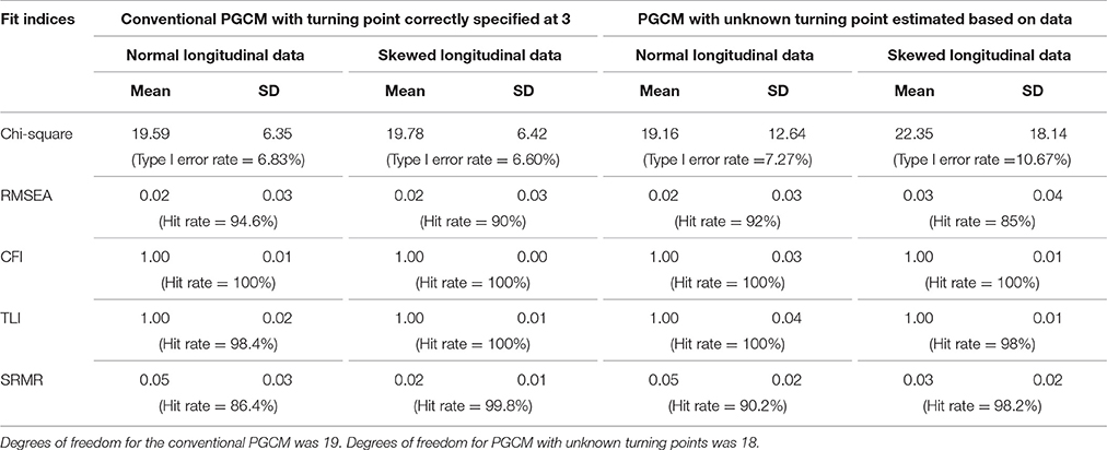
Table 2. Descriptive statistics of fit indices when the true turning point was at time point 3.

For the newly proposed PGCM, the Type I error rate was 7.27% when distributions were normal, which was lower than that for the skewed distributions (Type I error rate = 10.67%). This suggests that the newly proposed PGCM could be sensitive to data distributions, and deviation from normality could result in higher rejection rate even when the model was appropriately specified.

Table 2 also presented the means and SDs of RMSEA, CFI, TLI, and SRMR, as well as their hit rates, which are the percentages of replications that correctly identified the true models. The means of RMSEA were below 0.06 across the conditions. The hit rates of the indexes were 94.6 and 92% respectively in both model specifications for normal distributions, and dropped to 90 and 85% when distributions were moderately skewed. Contrarily, the hit rates of SRMR were 86.4 and 90.2% in both models for normal distributions but increased substantially to almost 100% for conventional PGCM and 98.2% for newly proposed PGCM when data distributions were moderately skewed. CFI and TLI had means of 1.0 and almost 100% in hit rates across all the conditions in the correctly specified model.

The means and SDs of the modification indices² (MI) as well as the percentage of the replications that had significant MI value associated with the targeted fixed parameters were presented in Table 3. Additional information summarized in Table 3 includes the range of SEPCs (the fully standardized Expected Parameter Changes) and the percentage of SEPCs larger than 0.2. The mean of MI ranged from 5.34 to 5.89 and the percentage of significant MI (≥7.88) ranged from 2.4 to 3.4% across the design factors. The range of SEPCs became narrower with the increase of sample size regardless of distributions and the change in growth rate. The percentages of SEPCs larger than 0.2 ranged from 0 to 4%.

TABLE 3

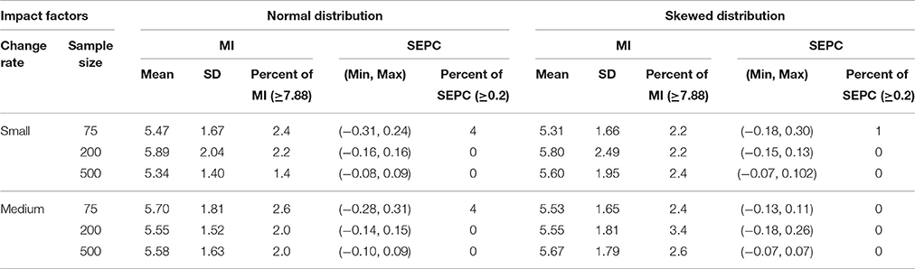
Table 3. Descriptive statistics of modification indices (MI) for the conventional PGCM with the turning point correctly specified to be at 3.

Performance of Fit Indexes in PGCMs with Mis-Specified Turning Points

Table 4 summarized the descriptive information for the χ² test statistic, RMSEA, SRMR, CFI, and TLI across all proper replications in conventional PGCMs when the turning point is mis-specified.

TABLE 4

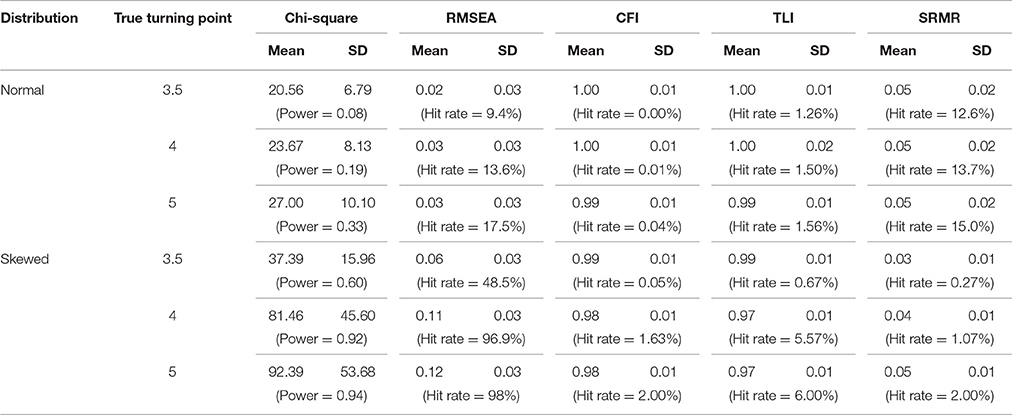
Table 4. Descriptive statistics of the chi-square test statistic and fit indices of the conventional PGCM with the turning point mis-specified to be at 3.

When distributions were normal, the means and SDs of the χ² test statistic increased from 20.56 and 6.79 to 27.00 and 10.10 as the degree of turning point misspecification increased from 0.5 to 2 time points. With skewed distributions, the changes were much greater, from 37.39 and 15.96 in mean and SD to 92.39 and 53.68 as the degree of turning point misspecification increased from 0.5 to 2 time points. The empirical power to detect turning point misspecification for normally distributed data was low (power = 0.33 with 2 time points misspecification). However, when distributions were moderately skewed, the empirical power to detect model misspecification reached 0.92 with 1 time point misspecification and 0.94 with 2 time point misspecification. It is suggestive that the misspecification of turning point was confounded with deviations from multivariate normality. The χ² test statistic detects the non-normality in the distribution, not necessarily the turning point misspecification.

As shown in Table 4, when distributions were normal, the means of RMSEA were below 0.06 (the cutoff criteria). The hit rates were small, ranging from 9.4, 13.6, to 17.5%, showing low sensitivity to turning point misspecification. However, when it came to skewed distributions, the means of RMSEA increased from 0.06 to 0.12 as the severity of misspecification increased from 0.5 to 2 time points. The same increase trend was observed for hit rates, increasing from 48.5% with 0.5 time point misspecification to 96.9 and 98% when the misspecification was by 1 or 2 time points respectively.

The means of CFI and TLI showed almost no deviation from 1.0 with very small SDs across all conditions. The hit rates of both CFI and TLI were close to 0 when distributions were normal and increased to about 6.00% when distributions are skewed, regardless of the increased severity in turning point misspecification. The performance of CFI and TLI was the least desirable in capturing the misspecification in turning point.

The means and SDs of SRMR remained the same (0.05, smaller than the cutoff value 0.08) across the different levels of severity in turning point misspecification with normal distributions. An increasing trend was observed in the hit rates with the increase of misspecification severity, but not to the extent of being effective in detecting the model misspecification. The hit rates in skewed data conditions were much smaller in size than the values in the conditions of normal distributions.

Table 5 summarized the performance of MI and SEPC in identifying the misspecification in conventional PGCM when the a priori turning point was mis-specified. Holding the severity of misspecification constant, the means of MI were found to increase with the increase of the sample size and with the change from normal distributions to skewed distributions. With normal distributions, the percentage of replications with MI exceeding the threshold of 7.88 ranged between 2.7% (0.5 time point misspecification with a sample size of 75) and 40.0% (2 time points misspecification with a sample size of 500). The percentage increased substantially when the distributions were moderately skewed.

TABLE 5

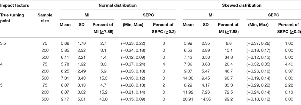
Table 5. Descriptive statistics of modification indices (MI) for the conventional PGCM with the turning point mis-specified to be at 3.

SEPC showed a pattern of increasingly narrower range with the increase of sample size after keeping the levels of severity in turning point misspecification constant. The percentages of replications with SEPC exceeding the threshold of 0.2 were below 5% across all conditions. Overall, SEPC based on MI was a poor indicator in detecting the mis-specified locations of turning points.

Standardized Bias of Fixed Effect Estimates

Table 6 presents the means of the standardized bias of fixed effect estimates for the correctly specified conventional PGCMs (i.e., the turning point was specified correctly a priori) and PGCMs with an unknown turning point estimated based on data when the true turning point is 3 in the population. On average, with conventional PGCMs, the standardized bias of fixed effect estimates of the Intercept (a), 1st Slope (b₁) and 2nd Slope (b₂) ranged from 0 to 0.08, negligibly small across the design factors. For PGCMs with unknown turning points, the standardized bias of fixed effect estimates a, b₁, and b₂ ranged from 0.00 to 0.32. Larger standardized biases were found under the normal distribution condition than the skewed distribution. This is counterintuitive; however, a closer examination revealed that the unstandardized biases were larger under the skewed distribution condition. The standardized biases looked smaller, because the standard deviations of the estimates were inflated under the skewed distribution.

TABLE 6

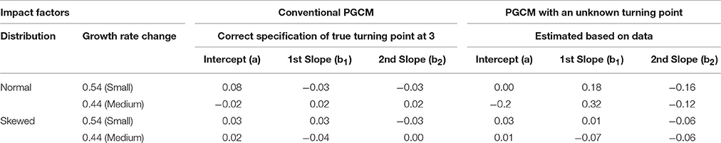
Table 6. Mean standardized biases of fixed effects when the true turning point was at time point 3.

The interaction between data distributions and change in growth rate explained a substantial amount of variation in the biases of the estimate of a (η² = 0.15) (see Figure 1A) and of b₁ (η² = 0.16) (see Figure 1B). The interaction effects between data distributions and sample size (η² = 0.13) (see Figure 2A) and between sample size and change rate (η² = 0.12) (see Figure 2B) were found to account significantly for the variations of the biases of the estimates of b_2.

FIGURE 1

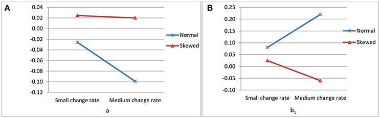
Figure 1. (A) Interaction effect between change in growth rate and data distributions on the standardized bias of the intercept (a) estimate and (B) Interaction effect between change in growth rate and data distributions on the bias of b₁ estimate.

FIGURE 2

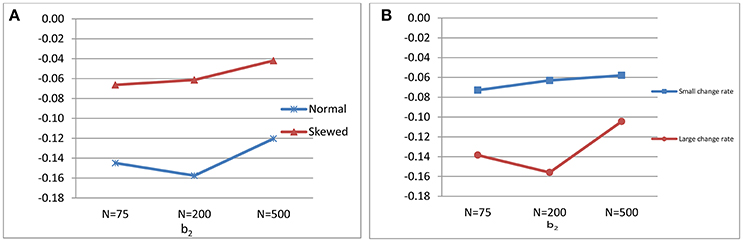
Figure 2. (A) Interaction effect between sample size and data distributions and (B) Interaction effect between sample size and change in growth rate on the standardized bias of b₂ estimate.

As summarized in Table 7, when the conventional PGCM was mis-specified due to the mislocation of the turning point, with normal distributions and a small change in growth rate, the biases of the estimate of a were acceptable regardless of the misspecification severity. However, the increase in misspecification severity from 0.5 to 2 time points led to an increase from 0.15 to 0.22 in the mean standardized bias for b₁ and from 0.23 to 1.19 for b₂. The biases were larger when the change in growth rate was medium, resulting in an increase in the bias from 0.31 to 0.77 for b₁ and from 0.66 to 3.16 for b₂, with increase in misspecification severity from 0.5 to 2 time points.

TABLE 7

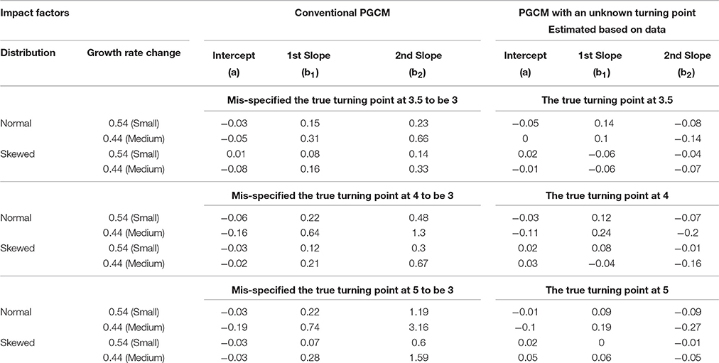
Table 7. Mean standardized biases of fixed effects when the true turning point was at 3.5, 4, or 5.

When distributions were skewed, the corresponding bias was mitigated to some degree but was still considered unacceptable particularly when the change in growth rate was medium. For example, the mean bias for b₂ increased from 0.33 to 1.59 with increase in misspecification severity from 0.5 to 2 time points. However, when using PGCM with unknown turning points, biases were considered small (about 0.20) for almost all fix effect estimates across almost all conditions in spite of the different distributions in the data.

ANOVA was used to partition the total variance in the standardized biases associated with the effects of the six design factors. Table 8 presented the eta-squared and the statistical significance of the main effects and interactions of the design factors on standardized bias. Statistically significant effects (p < 0.05) were marked with asterisks and were bolded if they were found to be practically significant (η² > 0.1). The design factors of data distributions (η² = 0.17) and change rate in growth (η² = 0.10) had substantial main effects on the bias of the mean of intercept (α). Data distribution was found to have substantial main effect (η² = 0.20), model specification and the level of severity in turning point misspecification were found to have significant interaction effects respectively on the bias associated with the estimates of b₁ (η² = 0.13) and with the mean of b₂ (η² = 0.17), as Figure 3A shows.

TABLE 8

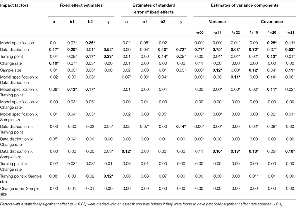
Table 8. Effect sizes of the impacts of the design factors on the standardized bias of estimated model parameters.

FIGURE 3

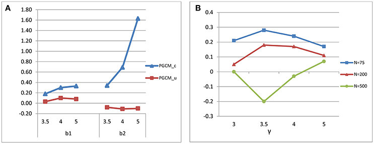
Figure 3. (A) Interaction effect between the locations of true turning point and model specification (Model Specification × Turning point) on the standardized bias of fixed effect estimate of b₁ and b₂. (B) Interaction effect between sample size and the locations of true turning point (Turning point × Sample size) on the standardized bias of turning point (γ) estimate in PGCM with unknown turning points.

Standardized Bias of Variance-Covariance Estimates

Table 9 shows the means of the standardized bias of variance components estimates broken down by model specification, distributions and sample size, the factors consistently found to be systematically related to the observed bias of the estimates of the variance components. When the fitting model was PGCM with unknown turning points, for normal data distributions, the mean biases of the estimated variance components were negligibly small, ranging from −0.03 to 0.15. On the other hand, when the fitted model was the conventional PGCM with mis-specified turning points, large biases were observed in the variance components estimates. The biases increased as sample size increased. For example, an increase of sample size from 75 to 500 led to an increase in the mean biases from 0.14 to 0.51 for τ_π11 and from −0.65 to −1.52 for τ_π22. In addition, when the data distributions were skewed, the variance components were highly biased for both models and in general the biases increased with the increase of sample size.

TABLE 9

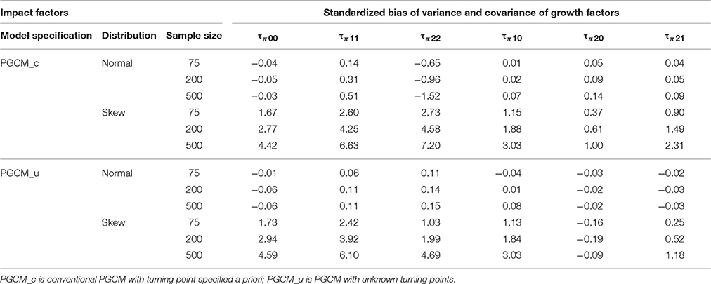
Table 9. Mean standardized biases of variance components estimates.

Bias of the Turning Point Estimates

The accuracy of the turning point estimates was examined using both the standardized and the unstandardized bias due to the practical meaning of the metric of time points. As summarized in Table 10, the maximum mean unstandardized bias was around 0.25 when sample size is 75, growth rate change is small, and distribution is normal, indicating that the estimated turning point is 0.25 time point away from the true turning point under those conditions. The minimum mean unstandardized bias was around 0.01 when sample size is 500, growth rate change is medium, and distribution is normal. Regardless of the locations of the true turning point, the mean unstandardized biases decreased with the increase in sample size and the increase in the change of growth rate (from small to medium). Though similar trends were observed with skewed distributions, the values of the unstandardized biases were much larger.

TABLE 10

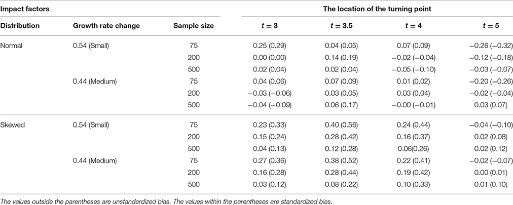
Table 10. Mean unstandardized and standardized biases of turning point (γ) estimates.

On the other hand, taking the variation in the turning point estimates into consideration, the standardized bias was much smaller under the normal distribution condition (η² = 0.52). An interaction effect was found between the location of the turning point and sample size (η² = 0.12). As shown in Figure 3B, the standardized biases were the smallest when the turning point was located at time point 4 and when the sample size was moderately large (N = 500).

Standardized Bias of Standard Errors of Fixed Effects and Turning Point Estimates for PGCM with Unknown Turning Point

Table 11 showed the means of the standardized bias of the SEs of fixed effect and turning point estimates for PGCM with unknown turning point. The mean standardized bias of SEs of a, b₁ and b₂ were negligibly small, ranging from 0.00 to 0.07 in absolute values. However, large biases were found in the SEs associated with the estimates of the turning point (γ). When the distributions were normal, the observed bias of the SEs of γ were acceptable, ranging from −0.03 to 0.26; when the distributions were skewed, the estimates of the SEs of γ were highly biased and underestimated with exception to the condition when the turning point was located at the 5th time point.

TABLE 11

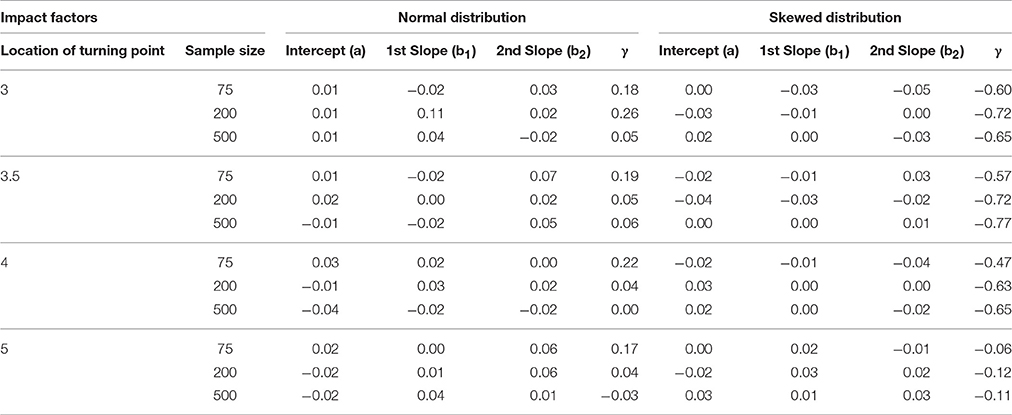
Table 11. Mean standardized biases of standard errors of fixed effects and turning point estimates.

As observed in Table 8, data distributions and sample size had statistically and practically significant interaction effect (η² = 0.12) on the observed bias of SEs of a. The SEs of b₂ were found to be substantially affected by data distribution (η² = 0.10) and the severity of turning point misspecification (η² = 0.14). Data distribution and the locations of the true turning point exhibited a significant interaction effect (η² = 0.14) on the bias of the SEs of the turning point (γ). The earlier the turning point is located at the time series, the larger the biases are associated with the estimates of the SEs of the turning point (γ), and such biases are even larger with moderately skewed data distributions.

Discussion

The study investigated the impacts of mis-specified turning point on growth trait estimation in conventional PGCMs that require turning points to be specified a priori. We examined the sensitivity of generally used model fit diagnostics [i.e., χ² test statistic, RMSEA, CFI, TLI, SRMR, modification index (MI), and SEPC] in detecting specification errors in conventional PGCMs due to turning points mislocation. In addition, the performance of an alternative procedure, PGCMs with unknown turning points (i.e., the turning point is treated as a parameter to be estimated based on data) was evaluated. The design factors considered in the simulation study were locations of true turning point (respectively at time point 3, 3.5, 4, or 5), sample size (75 or 200 or 500), and data distributions (normal vs. moderately skewed). This section summarized and discussed the results of the study.

Impact of Turning Point Misspecification

Misspecification of the turning point in conventional PGCM was found to have a substantial impact on the fixed effects estimates of 1st Slope (b₁) and 2nd Slope (b₂). The biases were considered acceptable only when the turning point was mis-specified by 0.5 time point with a small change in growth rate between the 1st and 2nd piece. Misspecification of a turning point earlier than its true location would result in overestimation of the growth rates in b₁ and b₂. Overall, the more severe the misspecification of the turning point is, the greater the impact is on the estimates, and the more misrepresented the growth trait estimates are for the population data. Such consequences are exacerbated when the change in growth rate is medium.

As expected, misspecification of the turning point also gives rise to unacceptably large biases with respect to the estimated variance components. The variances of the slopes of the 1st and 2nd piece are underestimated, with the latter being more severely underestimated. Since the variance of the slope factors reflects inter-individual differences in growth rates, the underestimation results may lead to the wrong conclusion that individuals have similar growth process. For applied researchers who are interested in using individual level predictors to predict the variation in growth rates, the deflated variance component estimates may attenuate the relationship between the predictors and growth rates, leading to misleading inferential conclusions.

Sensitivity of Model Fit Index Diagnostics

An optimal identification of the location of a turning point a priori is important for conventional PGCMs. When the location of a turning point was mis-specified in conventional PGCMs, our simulation results indicated that the model fit indices [i.e., χ² test statistic, RMSEA, CFI, TLI, SRMR, modification index (MI), and SEPC], generally did not perform effectively in detecting the misspecification errors. The performance of the overall model χ² test was not only affected by the severity of misspecification in turning point but also by the incidental characteristics of the data (e.g., data distributions, sample size). The magnitude of χ² test statistic increased as the distribution changes from normal to skewed and with the increase in sample size. Such undesirable characteristics of χ² test statistic were already confirmed in many studies (see e.g., [35, 45–47]). Additionally, χ² test statistic showed a lack of adequate power to detect model misspecification in almost all conditions with exception to conditions where the data distributions were moderately skewed and severity in misspecification was by 1 time point or more.

As a function of χ², RMSEA performed similarly as χ² test statistic. RMSEA was not sensitive to the degree of misspecification in turning point when distributions were normal. Similar to χ² test statistic, it was found to be relatively more effective only when distributions were moderately skewed and the turning point was mis-specified by 1 or more time points. However, such seemingly high power of RMSEA in non-normal distributions should be taken with caution, as warned by Nevitt and Hancock [48], the apparent advantage of high power of RMSEA is a result of the inflated χ² test statistic when multivariate normality is violated. Nor were CFI, TLI, and SRMR effective in capturing the misspecifications under any of the design conditions. Although previous studies showed that the three fit indices are effective in detecting the specification error when a piecewise growth trajectory is mis-specified as linear (see [27, 28]), our study shows that the three fit indices do not work well when the misspecification is on the location of the turning point rather than the linearity of the trajectory.

The findings with regards to the performance of the MI and the SEPC showed that MI tended to be more accurate in skewed distributions particularly in conditions where the severity in turning point misspecification was by at least 1 time point and the sample size was moderately large (N = 500). It is not surprising that the performance of modification indices are also influenced by data distributions; modification index is a function of χ² test, basically a univariate delta χ² tests computed on each fixed parameter if freely estimated. Contrary to the recommendation of Saris et al. [35] that an SEPC ≥ 0.2 indicates a substantial misspecification, we found that SEPC was a poor indicator of turning point misspecification in PGCM.

Performance of PGCM with Unknown Turning Points

Overall, the PGCM with unknown turning points was found to perform very well in recovering the fixed effects and the random effects when the longitudinal responses follow a multivariate normal distribution. However, when data distributions deviate from normality, relatively large biases were found to be associated with the standard error estimates of the turning point and the random effects of growth factors. The biases of the turning point estimates are small to moderate in general. It is interesting that when the location of the turning point is at time point 4, the estimation of the turning point becomes highly accurate regardless of data distribution types. This finding to some degree corresponds to the results in Kohli and Harring's [5] study which showed that the locations of the turning point were systematically related to the relative bias of growth parameters, particularly with the estimation of the mean of the slope of the 2nd piece. Specifically, the earlier the turning point is located in the time series, the larger the bias is. However, their study differed from ours in two major aspects: their population model was a second-order piecewise latent growth curve model; though they evaluated the model performance in the recovery of growth parameters with regards to the estimation of the intercept, slopes of the 1st and 2nd piece, the focus was not on the estimation of the turning point and therefore, no relevant findings were discussed in their study.

Recommendations

In longitudinal data analysis, if a turning point is hypothesized at a specific time point, applied researchers tend to specify an a priori piecewise linear model to capture the turning point and examine whether the model fits the data. The simplest approach to evaluate model fit is through the use of model fit indices and MIs, however, the present findings showed that those generally used model fit diagnostics are not accurate or effective in detecting specification errors related to the turning point location. Unless the misspecification is severe (i.e., by at least 1 time point) and the longitudinal data follow a multivariate moderately skewed distribution, the generally used fit indices are not able to identify the specification errors.

If a turning point is hypothesized but its location is unknown, the MI-based procedure proposed by Kwok et al. [6] can be used to fit a linear growth curve model in the data and then identify largest MI for factor loadings of the linear growth factor; however, the procedure requires moderately large sample size (400 and above) and more measurement waves (minimally 8 waves in the study) to have adequate statistical power to detect the turning point. A more powerful alternative to the MI-procedure is the piecewise linear model with unknown turning points estimated based on data. The present findings regarding the performance of the procedure in recovering the mean growth trajectory showed the estimation is highly accurate even if the multivariate normality assumption is violated. Applied researchers are recommended to take advantage of the procedure to correctly identify the turning point in specifying a piecewise linear growth model. Yet, for applied researchers who are interested in the significance test of the turning point and/or the interindividual difference, it is cautioned that the departure from multivariate normality assumption in longitudinal responses tend to inflate the standard error estimates of the turning point and deflate the random effect estimates associated with the growth factors.

Limitations and Future Research Directions

The findings of the study should be considered in light of the limitations and may not be generalized to models and data scenarios that are very different from the ones considered in this study. A limitation to be considered in generalizing the findings of the study is with respect to the level of change in growth rate. As a matter of fact, the change in growth rate can be much larger than what has been considered in our study (e.g., in Kohli and Harring's [5] study, the resulted effect size from the change in growth rate is 5). Another limitation to be considered is that we only examined the impact of a mis-specified turning point on growth trait estimation in a priori piecewise linear model, assuming all other parts of the latent growth model were correctly specified. Yet, in real data scenarios, the misspecification of turning point can happen simultaneously with misspecifications in the other parts of the latent growth model (e.g., the misspecification of residual variances across the measurement waves often happens). How the misspecifications in both the turning point and other parts of the latent growth model interact with the design factors considered in present study particularly when the normal distributions were violated is another question that merits research attention.

Finally, the study only considered two-piece linear growth curves connected by one fixed turning point. In reality, developmental trajectories may have a zigzag shape with multiple turning points. In addition, there might be individual differences in the location of the turning points. Hence, further development of the PGCM is needed to model trajectories with multiple unknown turning points and random effects associated with the turning points.

Author Contributions

LN and WL jointly conceived and designed the study. LN acquired the data, conducted the analysis and interpretation of the data with the help of WL. LN drafted the manuscript with the conceptual advice from WL. LN and WL worked jointly in revising the manuscript critically for important intellectual content and for the final approval of the version to be published and for the accountability for all aspects of the work to ensure that the questions related to the accuracy or integrity of any part of the work are appropriately investigated and resolved.

Conflict of Interest Statement

The authors declare that the research was conducted in the absence of any commercial or financial relationships that could be construed as a potential conflict of interest.

The reviewer KJK and handling Editor declared their shared affiliation.

Acknowledgments

The open access publishing fees for this article have been covered in part by the Texas A&M University Open Access to Knowledge Fund (OAKFund), supported by the University Libraries and the Office of the Vice President for Research. The Center for Student Affairs Assessment at University of California, Davis, has also contributed partly to the publishing fees for this article.

Footnotes

1. ^Where $\widehat{\theta }$ is the parameter estimate, θ the population parameter value, and $S(\widehat{\theta })$ the standard deviation of the estimates across 500 replications.

2. ^MI is not available in Mplus for the PGCM with unknown turning points due to nonlinear constraints in fitting the model.

References

1. Preacher KJ, Wichman AL, MacCallum RC, Briggs NE. Latent Growth Curve Modeling. Los Angeles, CA: Sage (2008).

Google Scholar

2. Singer JD, Willett JB. Applied Longitudinal Data Analysis: Modeling Change and Event Occurrence. New York, NY: Oxford University Press (2003).

Google Scholar

3. Harring JR, Cudeck R, du Toit SH. Fitting partially nonlinear random coefficient models as SEMs. Multivariate Behav Res. (2006) 41:579–96. doi: 10.1207/s15327906mbr4104_7

PubMed Abstract | CrossRef Full Text | Google Scholar

4. Khoo S, West SG, Wu W, Kwok O. Longitudinal Methods. In: Eid M, Diener E, editors. Handbook of Psychological Measurement: A Multimethod Perspective. Washington, DC: APA (2006). p. 301–17.

Google Scholar

5. Kohli N, Harring JR. Modeling growth in latent variables using a piecewise function. Multivariate Behav. Res. (2013) 48:370–97. doi: 10.1080/00273171.2013.778191

PubMed Abstract | CrossRef Full Text | Google Scholar

6. Kwok O, Luo W, West SG. Using modification indexes to detect turning points in longitudinal data: a monte carlo study. Struct Equ Model. (2010) 17:216–40. doi: 10.1080/10705511003659359

CrossRef Full Text | Google Scholar

7. Chou C, Yang D, Pentz MA, Hser Y. Piecewise growth curve modeling approach for longitudinal prevention study. Comput Stat Data Anal. (2004) 46:213–25. doi: 10.1016/S0167-9473(03)00149-X

CrossRef Full Text | Google Scholar

8. Rutter M. Autism research: prospects and priorities. J Autism Dev Disord. (1996) 26:257–75. doi: 10.1146/annurev.psych.52.1.501

PubMed Abstract | CrossRef Full Text | Google Scholar

9. Hardy SA, Thiels C. Using latent growth curve modeling in clinical treatment research: an example comparing guided self-change and cognitive behavioral therapy treatments for bulimia nervosa. Int J Clin Health Psychol. (2009) 9:51–71. doi: 10.1016/j.eurpsy.2007.01.590

CrossRef Full Text | Google Scholar

10. Terrera GM, Matthews F, Brayne C. A comparison of parametric models for the investigation of the shape of cognitive change in the older population. BMC Neurol. (2008) 8:16. doi: 10.1186/1471-2377-8-16

PubMed Abstract | CrossRef Full Text | Google Scholar

11. Dominicus A, Ripatti S, Pedersen N, Palmgren J. Modelling Variability in Longitudinal Data Using Random Change Point Models. Research Reports in Mathematical Statistics. Stockholm University (2006). Available online at: http://www.math.su.se/matstat

Google Scholar

12. Wang L, McArdle JJ. A simulation study comparison of Bayesian estimation with conventional methods for estimating unknown change points. Struct Equ Model. (2008) 15:52–74. doi: 10.1080/10705510701758265

CrossRef Full Text | Google Scholar

13. Wood PK, Jackson KM. Escaping the snare of chronological growth and launching a free curve alternative: general deviance as latent growth model. Dev Psychopathol. (2013) 25:739–54. doi: 10.1017/S095457941300014X

PubMed Abstract | CrossRef Full Text | Google Scholar

14. Preacher KJ, Hancock GR. Meaningful aspects of change as novel random coefficients: a general method for reparameterizing longitudinal models. Psychol Methods (2015) 20:84. doi: 10.1037/met0000028

PubMed Abstract | CrossRef Full Text | Google Scholar

15. Wu W, Jia F, Kinai R, Little TD. Optimal number and allocation of data collection points for linear spline growth curve modeling: a search for efficient designs. Int J Behav Dev. (2019) 41:550–58. doi: 10.1177/0165025416644076

CrossRef Full Text | Google Scholar

16. Compton DL, Fuchs LS, Fuchs D, Lambert W, Hamlett C. The cognitive and academic profiles of reading and mathematics learning disabilities. J Learn Disabil. (2012) 45:79–95. doi: 10.1177/0022219410393012

PubMed Abstract | CrossRef Full Text | Google Scholar

17. Steiger JH. Structural model evaluation and modification: an interval estimation approach. Multivariate Behav. Res. (1990) 25:173–80. doi: 10.1207/s15327906mbr2502_4

PubMed Abstract | CrossRef Full Text | Google Scholar

18. Jöreskog KG, Sörbom D. LISREL 7: A Guide to the Program and Applications. Chicago, IL: SPSS (1988).

19. Bentler PM. Comparative fit indexes in structural models. Psychol. Bull. (1990) 107:238–46. doi: 10.1037/0033-2909.107.2.238

PubMed Abstract | CrossRef Full Text | Google Scholar

20. Tucker LR, Lewis C. A reliability coefficient for maximum likelihood factor analysis. Psychometrika (1973) 38:1–10. doi: 10.1007/BF02291170

CrossRef Full Text | Google Scholar

21. Hu L, Bentler PM. Fit indices in covariance structure analysis: sensitivity to underparameterized model misspecification. Psychol Methods (1998) 3:424–53. doi: 10.1037/1082-989X.3.4.424

CrossRef Full Text | Google Scholar

22. Hu L, Bentler PM. Cutoff criterion for fit indexes in covariance structure analysis: conventional criteria versus new alternatives. Struct Equ Model. (1999) 6:1–55. doi: 10.1080/10705519909540118

CrossRef Full Text | Google Scholar

23. Fan X, Sivo SA. Sensitivity of fit indexes to mis-specified structural or measurement model components: rationale of two-index strategy revisited. Struct Equ Model (2005) 12:343–67. doi: 10.1207/s15328007sem1203_1

CrossRef Full Text | Google Scholar

24. Fan X, Sivo SA. Sensitivity of fit indices to model misspecification and model types. Multivariate Behav. Res. (2007) 42:509–29. doi: 10.1080/00273170701382864

CrossRef Full Text | Google Scholar

25. Chen F, Curran PJ, Bollen KA, Kirby J, Paxton P. An empirical evaluation of the use of fixed cutoff points in RMSEA test statistic in structural equation models. Sociol. Methods Res. (2008) 36:462–94. doi: 10.1177/0049124108314720

PubMed Abstract | CrossRef Full Text | Google Scholar

26. Wu W, West SG, Taylor AB. Evaluating model fit for growth curve models: integration of fit indices from SEM and MLM frameworks. Psychol. Methods (2009) 14:183. doi: 10.1037/a0015858

PubMed Abstract | CrossRef Full Text | Google Scholar

27. Wu W, West SG. Sensitivity of fit indices to misspecification in growth curve models. Multivariate Behav. Res. (2010) 45:420–52. doi: 10.1080/00273171.2010.483378

PubMed Abstract | CrossRef Full Text | Google Scholar

28. Leite WL, Stapleton LM. Detecting growth shape misspecifications in latent growth models: an evaluation of fit indexes. J Exp Educ. (2011) 79:361–81. doi: 10.1080/00220973.2010.509369

CrossRef Full Text | Google Scholar

29. Widaman KF, Thompson JS. On specifying the null model for incremental fit indices in structural equation modeling. Psychol Methods (2003) 8:16–37. doi: 10.1037/1082-989X.8.1.16

PubMed Abstract | CrossRef Full Text | Google Scholar

30. Hutchinson SR. Univariate and multivariate specification search indices in covariance structure modeling. J Exp Educ. (1993) 61:171–81. doi: 10.1080/00220973.1993.9943859

CrossRef Full Text | Google Scholar

31. Saris WE, Satorra A, Sörbom D. The detection and correction of specification errors in structural equation models. In: Clogg CC, editor, Sociological Methodology, San Francisco, CA: Jossey-Bass (1987). p. 105–129.

Google Scholar

32. Kaplan D. The impact of specification error on the estimation, testing, improvement of structural equation models. Multivariate Behav Res. (1988) 23:69–86. doi: 10.1207/s15327906mbr2301_4

PubMed Abstract | CrossRef Full Text | Google Scholar

33. Chou CP, Bentler PM. Invariant standardized estimated parameter change for model modification in covariance structure analysis. Multivariate Behav. Res. (1993) 28:97–110. doi: 10.1207/s15327906mbr2801_6

PubMed Abstract | CrossRef Full Text | Google Scholar

34. Whittaker TA. Using the modification index and standardized expected parameter change for model modification. J Exp Educ. (2012) 80:26–44. doi: 10.1080/00220973.2010.531299

CrossRef Full Text | Google Scholar

35. Saris WE, Satorra A, Van der Veld WM. Testing structural equation models or detection of misspecifications?. Struct Equ Model. (2009) 16:561–82. doi: 10.1080/10705510903203433

CrossRef Full Text | Google Scholar

36. Chou CP, Bentler PM. Model modification in covariance structure modeling: a comparison among likelihood ratio, lagrange multiplier, Wald tests. Multivariate Behav Res. (1990) 25:115–36. doi: 10.1207/s15327906mbr2501_13

PubMed Abstract | CrossRef Full Text | Google Scholar

37. Luijben TC, Boomsma A. Statistical guidance for model modification in covariance structure analysis. Compstat (1988) 1988:335–40. doi: 10.1007/978-3-642-46900-8_46

CrossRef Full Text | Google Scholar

38. MacCallum RC. Specification searches in covariance structure modeling. Psychol. Bull. (1986) 100:107–20. doi: 10.1037/0033-2909.100.1.107

PubMed Abstract | CrossRef Full Text | Google Scholar

39. Raudenbush SW, Liu XF. Effects of study duration, frequency of observation, and sample size on power in studies of group differences in polynomial change. Psychol. Methods (2001) 6:387. doi: 10.1037/1082-989X.6.4.387

PubMed Abstract | CrossRef Full Text | Google Scholar

40. Vale CD, Maurelli VA. Simulating multivariate nonnormal distributions. Psychometrika (1983) 48:465–71. doi: 10.1007/BF02293687

CrossRef Full Text | Google Scholar

41. Micceri T. The unicorn, the normal curve, and other improbable creatures. Psychol Bull. (1989) 105:156. doi: 10.1037/0033-2909.105.1.156

CrossRef Full Text | Google Scholar

42. Bauer DJ, Curran PJ. Distributional assumptions of growth mixture models: implications for overextraction of latent trajectory classes. Psychol Methods (2003) 8:338. doi: 10.1037/1082-989X.8.3.338

PubMed Abstract | CrossRef Full Text | Google Scholar

43. SAS Institute (2016). SAS, Release 9.4 [Computer software]. Cary, NC: SAS Institute.

44. Muthén LK, Muthén BO. M plus User's Guide Seventh Edition. (1998–2016). Los Angeles, CA: Muthén & Muthén.

45. Boomsma A. On the Robustness of LISREL (Maximum Likelihood Estimation) Against Small Sample Size and Non-Normality. Doctoral dissertation, University of Groningen (1983).

Google Scholar

46. McIntosh CN. Rethinking fit assessment in structural equation modeling: a commentary and elaboration on Barrett (2007). Pers Individ Diff. (2007) 42:859–67. doi: 10.1016/j.paid.2006.09.020

CrossRef Full Text | Google Scholar

47. Yuan K. Fit indices versus test statistics. Multivariate Behav Res. (2005) 40:115–48. doi: 10.1207/s15327906mbr4001_5

PubMed Abstract | CrossRef Full Text | Google Scholar

48. Nevitt J, Hancock GR. Improving the root mean square error of approximation for nonnormal conditions in structural equation modeling. J Exp Educ. (2000). 68:251–68. doi: 10.1080/00220970009600095

CrossRef Full Text | Google Scholar

Appendix

Mplus Code for Fitting Newly Proposed PGCM with an Unknown Turning Point

Title: Newly Proposed PGCM;

Data:

     File is “C:\tpoint_4\data.txt”;

Variable:

     Names are ID t1-t7;

     Usevariables are t1-t7;

Analysis: Estimator=MLR;

MODEL:

     w1 BY t1-t7@1;

     w2 BY t1@0 t2@1 t3@2 t4@3 t5@4 t6@5 t7@6;

     w3 BY t1*0 (p1);

     w3 BY t2-t7 (p2-p7);

     w1; w2; w3;

     w1 WITH w2*0;

     w1 WITH w3*0;

     w2 WITH w3*0;

     [t1-t7@0];

     t1-t7*1;

     [w1](mw11);

     [w2](mw21);

     [w3](mw31);

MODEL CONSTRAINT:

       NEW(gam1*2.5 b11*2.0 b21*0.5 b41*0.3); ! The starting values set to be around the true values;

     p1 = (sqrt((0-gam1)^∧2));

     p2 = (sqrt((1-gam1)^∧2));

     p3 = (sqrt((2-gam1)^∧2));

     p4 = (sqrt((3-gam1)^∧2));

     p5 = (sqrt((4-gam1)^∧2));

     p6 = (sqrt((5-gam1)^∧2));

     p7 = (sqrt((6-gam1)^∧2));

     b11 = mw11+mw31*gam1;

     b21 = mw21−mw31;

     b41 = mw21+mw31;

OUTPUT: