When Is Network Lasso Accurate?

1. Introduction

In many applications ranging from image processing, social networks to bioinformatics, the observed datasets carry an intrinsic network structure. Such datasets can be represented conveniently by signals defined over a “data graph” which models the network structure inherent to the dataset [1, 2]. The nodes of this data graph represent individual data points which are labeled by some quantity of interest, e.g., the class membership in a classification problem. We represent this label information as a graph signal whose value for a particular node is given by its label [1, 3–8]. This graph signal representation of datasets allows to apply efficient methods from graph signal processing (GSP) which are obtained, in turn, by extending established methods (e.g., fast filtering and transforms) from discrete time signal processing (over chain graphs) to arbitrary graphs [9–11].

The resulting graph signals are typically clustered, i.e., these signals are nearly constant over well connected subset of nodes (clusters) in the data graph. Exploiting this clustering property enables the accurate recovery of graph signals from few noisy samples. In particular, using the total variation to measure how well a graph signal conforms with the underlying cluster structure, the authors of Hallac et al. [12] obtain the network Lasso (nLasso) by adapting the well-known Lasso estimator which is widely used for learning sparse models [13, 14]. The nLasso can be interpreted as an instance of the regularized empirical risk minimization principle, using total variation of a graph signal for the regularization. Some applications where the use of nLasso based methods has proven beneficial include housing price prediction and personalized medicine [12, 15].

A scalable implementation of the nLasso has been obtained via the alternating direction method of multipliers (ADMM) [16]. However, the authors of Boyd et al. [16] do not discuss conditions on the underlying network structure which ensure success of the network Lasso. We close this gap in the understanding of the performance of network Lasso, by deriving sufficient conditions on the data graph (cluster) structure and sampling set such that nLasso is accurate. To this end, we introduce a simple model for clustered graph signals which are constant over well connected groups or clusters of nodes. We then define the notion of resolving sampling sets, which relates the cluster structure of the data graph to the sampling set. Our main contribution is an upper bound on the estimation error obtained from nLasso when applied to resolving sampling sets. This upper bound depends on two numerical parameters which quantify the connectivity between sampled nodes and cluster boundaries.

Much of the existing work on recovery conditions and methods for graph signal recovery (e.g., [17–22]), relies on spectral properties of the data graph Laplacian matrix. In contrast, our approach is based directly on the connectivity properties of the underlying network structure. The closest to our work is Sharpnack et al. [23] and Wang et al. [24], which provide sufficient conditions such that a special case of the nLasso (referred to as the “edge Lasso”) accurately recovers piece-wise constant (or clustered) graph signals from noisy observations. However, these works require access to fully labeled datasets, while we consider datasets which are only partially labeled (as it is typical for machine learning applications where label information is costly).

1.1. Outline

The problem setting considered is formalized in section 2. In particular, we show how to formulate the problem of learning a clustered graph signal from a small amount of signal samples as a convex optimization problem, which is underlying the nLasso method. Our main result, i.e., an upper bound on the estimation error of nLasso is stated in section 3. Numerical experiments which illustrate our theoretical findings are discussed in section 4.

1.2. Notation

We will conform to standard notation of linear algebra as used, e.g., in Golub and Van Loan [25]. For a binary variable b, we denote its negation as $\bar{b}$.

2. Problem Formulation

We consider datasets which are represented by a network model, i.e., a data graph ${G}=({V},{E},\text{W})$ with node set ${V}=\left\{1,\dots ,N\right\}$, edge set ${E}$ and weight matrix $\text{W}\in {ℝ}_{+}^{N\times N}$. The nodes ${V}$ of the data graph represent individual data points. For example, the node $i\in {V}$ might represent a (super-)pixel in image processing, a neuron of a neural network [26] or a social network user profile [27].

Many applications naturally suggest a notion of similarity between individual data points, e.g., the profiles of befriended social network users or grayscale values of neighboring image pixels. These domain-specific notions of similarity are represented by the edges of the data graph ${G}$, i.e., the nodes $i,j\in {V}$ representing similar data points are connected by an undirected edge $\left\{i,j\right\}\in {E}$. We denote the neighborhood of the node $i\in {V}$ by ${N}(i):=\left\{j\in {V}:\left\{i,j\right\}\in {E}\right\}$. It will be convenient to associate with each undirected edge {i, j} a pair of directed edges, i.e., (i, j) and (j, i). With slight abuse of notation we will treat the elements of the edge set ${E}$ either as undirected edges {i, j} or as pairs of two directed edges (i, j) and (j, i).

In some applications it is possible to quantify the extent to which data points are similar, e.g., via the physical distance between neighboring sensors in a wireless sensor network application [28]. Given two similar data points $i,j\in {V}$, which are connected by an edge $\left\{i,j\right\}\in {E}$, we will quantify the strength of their connection by the edge weight W_{i, j} > 0 which we collect in the symmetric weight matrix $\text{W}\in {ℝ}_{+}^{N\times N}$. The absence of an edge between nodes $i,j\in {V}$ is encoded by a zero weight W_{i, j} = 0. Thus the edge structure of the data graph ${G}$ is fully specified by the support (locations of the non-zero entries) of the weight matrix W.

2.1. Graph Signals

Beside the network structure, encoded in the data graph ${G}$, datasets typically also contain additional labeling information. We represent this additional label information by a graph signal defined over ${G}$. A graph signal x[·] is a mapping ${V}\to ℝ$, which associates every node $i\in {V}$ with the signal value x[i]∈ℝ (which might representing a label characterizing the data point). We denote the set of all graph signals defined over a graph ${G}=({V},{E},\text{W})$ by ${ℝ}^{{V}}$.

Many machine learning methods for network structured data rely on a “cluster hypothesis” [4]. In particular, we assume the graph signals x[·] representing the label information of a dataset conforms with the cluster structure of the underlying data graph. Thus, any two nodes $i,j\in {V}$ out of a well-connected region (“cluster”) of the data graph tend to have similar signal values, i.e., x[i] ≈ x[j]. Two important application domains where this cluster hypothesis has been applied successfully are digital signal processing where time samples at adjacent time instants are strongly correlated for sufficiently high sampling rate (cf. Figure 1A) as well as processing of natural images whose close-by pixels tend to be colored likely (cf. Figure 1B). The cluster hypothesis is verified also often in social networks where the clusters are cliques of individuals having similar properties (cf. Figure 1C and Newman [29, Chap. 3]).

FIGURE 1

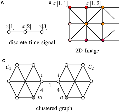
Figure 1. Graph signals defined over (A) a chain graph (representing, e.g., discrete time signals), (B) grid graph (representing, e.g., 2D-images) and (C) a general graph (representing, e.g., social network data), whose edges $\left\{i,j\right\}\in {E}$ are captioned by edge weights W_{i, j}.

In what follows, we quantify the extend to which a graph signal $x\left[·\right]\in {ℝ}^{{V}}$ conforms with the clustering structure of the data graph ${G}=({V},{E},\text{W})$ using its total variation (TV)

$\begin{array}{ll}\Vert x[·]{\Vert }_{\text{TV}}:={\displaystyle \sum _{\{i,j\}\in {E}}{W}_{i,j}}|x[j]-x[i]|.& (1)\end{array}$

For a subset of edges ${S}\subseteq {E}$, we use the shorthand

$\begin{array}{ll}\Vert x[·]{\Vert }_{{S}}:={\displaystyle \sum _{\{i,j\}\in {S}}{W}_{i,j}}|x[j]-x[i]|.& (2)\end{array}$

For a supervised machine learning application, the signal values x[i] might represent class membership in a classification problem or the target (output) value in a regression problem. For the house price example considered in Hallac et al. [12], the vector-valued graph signal x[i] corresponds to a regression weight vector for a local pricing model (used for the house market in a limited geographical area represented by the node i).

Consider a partition ${F}=\left\{{{C}}_1,\dots ,{{C}}_{\left|{F}\right|}\right\}$ of the data graph ${G}$ into $\left|{F}\right|$ disjoint subsets ${{C}}_l$ of nodes (“clusters”) such that ${V}={\bigcup }_{l=1}^{\left|{F}\right|}{{C}}_l$. We associate a subset ${C}\subseteq {V}$ of nodes with a particular “indicator” graph signal

$\begin{array}{ll}{{I}}_{{C}}[i]:=\{\begin{array}{ll}1\hfill & \text{ if }i\in {C}\hfill \\ 0\hfill & \text{ else}\text{.}\hfill \end{array}& (3)\end{array}$

A simple model of clustered graph signals is then obtained by piece-wise constant or clustered graph signals of the form

$\begin{array}{ll}x[i]={\displaystyle \sum _{l=1}^{|{F}|}{a}_l{{I}}_{{{C}}_l}[i].}& (4)\end{array}$

In Figure 2, we depict a clustered graph signal for a chain graph with 10 nodes which are partitioned into two clusters: ${{C}}_1$ and ${{C}}_2$.

FIGURE 2

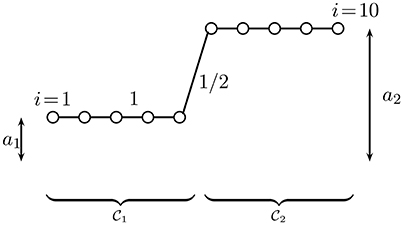
Figure 2. A clustered graph signal $x\left[i\right]=a_1{{I}}_{{{C}}_1}\left[i\right]+a_2{{I}}_{{{C}}_2}\left[i\right]$ (cf. Equation 4) defined over a chain graph which is partitioned into two equal-size clusters ${{C}}_1$ and ${{C}}_2$ which consist of consecutive nodes. The edges connecting nodes within the same cluster have weight 1, while the single edge connecting nodes from different clusters has weight 1/2.

It will be convenient to define, for a given partition ${F}$, its boundary $\partial {F}\subseteq {E}$ as the set of edges $\left\{i,j\right\}\in {E}$ which connect nodes $i\in {{C}}_a$ and $j\in {{C}}_b$ from different clusters, i.e., with ${{C}}_a\ne {{C}}_b$. With a slight abuse of notation, we will use the same symbol $\partial {F}$ also to denote the set of nodes which are connected to a node from another cluster.

The TV of a clustered graph signal of the form (Equation 4) can be upper bounded as

$\begin{array}{ll}\Vert x[·]{\Vert }_{\text{TV}}\le 2\underset{l\in \{1,\dots ,|{F}|\}}{\max }|a_l|{\displaystyle \sum _{\{i,j\}\in \partial {F}}{W}_{i,j}}.& (5)\end{array}$

Thus, for a partition ${F}$ with small weighted boundary $\sum _{\left\{i,j\right\}\in \partial {F}}{W}_{i,j}$, the associated clustered graph signals (Equation 4) have small TV ||x[·]||_TV due to Equation (5).

The signal model (Equation 4), which also has been used in Sharpnack et al. [23] and Wang et al. [24], is closely related to the stochastic block model (SBM) [30]. Indeed, the SBM is obtained from Equation (4) by choosing the coefficients $a_{{C}}$ uniquely for each cluster, i.e., $a_{{C}}\in \left\{1,\dots ,\left|{F}\right|\right\}$. Moreover, the SBM provides a generative (stochastic) model for the edges within and between the clusters ${{C}}_l$.

We highlight that the clustered signal model (Equation 4) is somewhat dual to the model of band-limited graph signals [1, 4–7, 17, 19]. The model of band-limited graph signals is obtained by the subspaces spanned by the eigenvectors of the graph Laplacian corresponding to the smallest (in magnitude) eigenvalues, i.e., the low-frequency components. Such band-limited graph signals are smooth in the sense of small values of the Laplacian quadratic form [31]

$\begin{array}{ll}{\displaystyle \sum _{\{i,j\}\in {E}}{W}_{i,j}}{(x[j]-x[i])}^2=x^{T}Lx.& (6)\end{array}$

Here, we used the vector representation x = (x[1], …, x[N])^T of the graph signal x[·] and the graph Laplacian matrix L ∈ ℝ^N×N defined element-wise as

$\begin{array}{ll}{L}_{i,j}=\{\begin{array}{ll}{\displaystyle {\sum }_{k\in {V}}{W}_{i,k}}\hfill & \text{ if }i=j\hfill \\ -W_{i,j}\hfill & \text{ otherwise}\text{.}\hfill \end{array}& (7)\end{array}$

A band-limited graph signal x[·] is characterized by a clustering (within a small bandwidth) of their graph Fourier transform (GFT) coefficients [22]

$\begin{array}{ll}\tilde{x}[l]:=u_l^{T}x,\text{ for }l=1,\dots ,N,& (8)\end{array}$

with the orthonormal eigenvectors ${\left\{{\text{u}}_l\right\}}_{l=1}^N$ of the graph Laplacian matrix L. In particular, by the spectral decomposition of the psd graph Laplacian matrix L (cf. Equation 7), we have L = UΛU^H with U = (u₁, …, u_N) and the diagonal matrix Λ having (in decreasing order) the non-negative eigenvalues λ_l of L on its diagonal.

In contrast to band-limited graph signals, a clustered graph signal of the form (Equation 4) will typically have GFT coefficients which are spread out over the entire (graph) frequency range. Moreover, while band-limited graph signals are characterized by having a sparse GFT, a clustered graph signal of the form (Equation 4) has a dense (non-sparse) GFT in general. On the other hand, while a clustered graph signal of the form (Equation 4) has sparse signal differences ${\left\{x\left[i\right]-x\left[j\right]\right\}}_{\left\{i,j\right\}\in {E}}$, the signal differences of a band-limited graph signal are dense (non-sparse).

Let us illustrate the duality between the clustered graph signal model (Equation 4) and the model of band-limited graph signals (cf. [7, 17]) by considering a dataset representing a finite length segment of a time series. The data graph ${{G}}_0$ underlying this time series data is chosen as a chain graph (cf. Figure 2), consisting of N = 100 nodes which represent the individual time samples. The time series is partitioned into two clusters ${{C}}_1,{{C}}_2$, each cluster consisting of 50 consecutive nodes (time samples). We model the correlations between successive time samples using edge weight W_{i, j} = 1 for data points i, j belonging to the same cluster and a smaller weight W_{i, j} = 1/2 for the single edge {i, j} connecting the two clusters ${{C}}_1$ and ${{C}}_2$.

A clustered graph signal (time series) $x_0\left[i\right]=a_1{{I}}_{{{C}}_1}\left[i\right]+a_2{{I}}_{{{C}}_2}\left[i\right]$ (cf. Equation 4) defined over ${{G}}_0$ is characterized by very sparse signal differences ${\left\{x_0\left[i\right]-x_0\left[j\right]\right\}}_{\left\{i,j\right\}\in {E}}$. Indeed the signal difference x₀[i] − x₀[j] of the clustered graph signal x₀[·] is non-zero only for the single edge {i, j} which connects ${{C}}_1$ and ${{C}}_2$. In stark contrast, the GFT of x₀[·] is spread out over the entire (graph) frequency range (cf. Figure 3), i.e., the graph signal x₀[·] does not conform with the band-limited signal model.

FIGURE 3

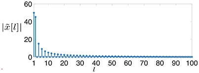
Figure 3. The magnitudes of the GFT coefficients $\tilde{x}\left[l\right]$ (cf. Equation 8) of a clustered graph signal x₀[·] defined over a chain graph (cf. Figure 2).

On the other hand, we illustrate in Figure 4 a graph signal x_BL[·] with GFT coefficients ${\tilde{x}}_{\text{BL}}\left[l\right]=1$ (cf. Equation 8) for l = 1, 2 and ${\tilde{x}}_{\text{BL}}\left[l\right]=0$ otherwise. Thus, the graph signal is clearly band-limited (it has only two non-zero GFT coefficients) but the signal differences x_BL[i] − x_BL[j] across the edges $\left\{i,j\right\}\in {E}$ are clearly non-sparse.

FIGURE 4

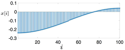
Figure 4. A band-limited graph signal defined over a chain graph with N = 100.

2.2. Recovery via nLasso

Given a dataset with data graph ${G}=({V},{E},\text{W})$, we aim at recovering a graph signal $x\left[·\right]\in {ℝ}^{{V}}$ from its noisy values

$\begin{array}{ll}y[i]=x[i]+e[i]& (9)\end{array}$

provided on a (small) sampling set

$\begin{array}{ll}{M}:=\{i_1,\dots ,i_M\}\subseteq {V}.& (10)\end{array}$

Typically M ≪ N, i.e., the sampling set is a small subset of all nodes in the data graph ${G}$.

The recovered graph signal $\widehat{x}\left[·\right]$ should incur only a small empirical (or training) error

$\begin{array}{ll}\widehat{E}(\widehat{x}[·]):={\displaystyle \sum _{i\in {M}}|}\widehat{x}[i]-y[i]|.& (11)\end{array}$

Note that the definition (Equation 11) of the empirical error involves the ℓ₁-norm of the deviation $\widehat{x}\left[·\right]i-y\left[i\right]$ between recovered and measured signal samples. This is different from the error criterion used in the ordinary Lasso, i.e., the squared-error loss $\sum _{i\in {M}}{(\widehat{x}\left[i\right]-y\left[i\right])}^2$ [32]. The definition (Equation 11) is beneficial for applications with measurement errors e_i (cf. Equation 9) having mainly small values except for a few large outliers [18, 33]. However, by contrast to plain Lasso, the error function in Equation (11) does not satisfy a restricted strong convexity property [34], which might be detrimental for the convergence speed of the resulting recovery methods (cf. Section 4).

In order to recover a clustered graph signal with a small TV $\left|\right|\widehat{x}\left[·\right]|{|}_{\text{TV}}$ (cf. Equation 5) from the noisy signal samples ${\left\{y\left[i\right]\right\}}_{i\in {M}}$ it is sensible to consider the recovery problem

$\begin{array}{ll}\widehat{x}[·]\in \underset{\tilde{x}[·]\in {ℝ}^{{V}}}{\text{arg}\text{min}}\widehat{E}(\tilde{x}[·])+\lambda \Vert \tilde{x}[·]{\Vert }_{\text{TV}}.& (12)\end{array}$

This recovery problem amounts to a convex optimization problem [35], which, as the notation already indicates, might have multiple solutions $\widehat{x}\left[·\right]$ (which form a convex set). In what follows, we will derive conditions on the sampling set ${M}$ such that any solution $\widehat{x}\left[·\right]$ of Equation (12) allows to accurately recover clustered a graph signal x[·] of the form (Equation 4).

Any graph signal obtained from Equation (12) balances the empirical error $\hat{E}(\widehat{x}\left[·\right])$ with the TV $\left|\right|\widehat{x}\left[·\right]|{|}_{\text{TV}}$ in an optimal manner. The parameter λ in Equation (12) allows to trade off a small empirical error against the amount to which the resulting signal is clustered, i.e., having a small TV. In particular, choosing a small value for λ enforces the solutions of Equation (12) to yield a small empirical error, whereas choosing a large value for λ enforces the solutions of Equation (12) to have small TV. Our analysis in section 3 provides a selection criterion for the parameter λ which is based on the location of the sampling set ${M}$ (cf. Equation 10) and the partition ${F}$ underlying the clustered graph signal model (Equation 4). Alternatively, for sufficiently large sampling sets one might choose λ using a cross-validation procedure [13].

Note that the recovery problem (Equation 12) is a particular instance of the generic nLasso problem studied in Hallac et al. [12]. There exist efficient convex optimization methods for solving the nLasso problem (Equation 12) (cf. [36] and the references therein). In particular, the alternating method of multipliers (ADMM) has been applied to the nLasso problem in Hallac et al. [12] to obtain a scalable learning algorithm which can cope with massive heterogeneous datasets.

3. When Is Network Lasso Accurate?

The accuracy of graph signal recovery methods based on the nLasso problem (Equation 12), depends on how close the solutions $\widehat{x}\left[·\right]$ of Equation (12) are to the true underlying graph signal $x\left[·\right]\in {ℝ}^{{V}}$. In what follows, we present a condition which guarantees any solution $\widehat{x}\left[·\right]$ of Equation (12) to be close to the underlying graph signal x[·] if it is clustered of the form (Equation 4).

A main contribution of this paper is the insight that the accuracy of nLasso methods, aiming at solving Equation (12), depends on the topology of the underlying data graph via the existence of certain flows with demands [37]. Given a data graph ${G}$, we define a flow on it as a mapping $h\left[·\right]:{V}\times {V}\to ℝ$ which assigns each directed edge (i, j) the value h[(i, j)], which can be interpreted as the amount of some quantity flowing through the edge (i, j) [37]. A flow with demands has to satisfy the conservation law

$\begin{array}{ll}{\displaystyle \sum _{j\in {N}(i)}h(j,i)-h(i,j)}=d[i],\text{ for any }i\in {V}& (13)\end{array}$

with a prescribed demand d[i] for each node $i\in {V}$. Moreover, we require flows to satisfy the capacity constraints

$\begin{array}{ll}|h(i,j)|\le W_{i,j}\text{ for any edge }(i,j)\in {E}\setminus \partial {F}.& (14)\end{array}$

Note that the capacity constraint (Equation 14) applies only to intra-cluster edges and does not involve the boundary edges $\partial {F}$. The flow values h(i, j) at the boundary edges $(i,j)\in \partial {F}$ take a special role in the following definition of the notion of resolving sampling sets.

Definition 1. Consider a dataset with data graph ${G}=({V},{E},\text{W})$ which contains the sampling set ${M}\subseteq {V}$. The sampling set ${M}$ resolves a partition ${F}=\left\{{{C}}_1,\dots ,{{C}}_{\left|{F}\right|}\right\}$ with constants K and L if, for any b_{i, j} ∈ {0, 1} with $\left\{i,j\right\}\in \partial {F}$, there exists a flow h[·] on ${G}$ (cf. Equations 13, 14) with

$\begin{array}{ll}h(i,j)=b_{i,j}·L·W_{i,j},h(j,i)={\overline{b}}_{i,j}·L·W_{i,j}& (15)\end{array}$

for every boundary edge $\left\{i,j\right\}\in \partial {F}$ and demands (cf. Equation 13) satisfying

$\begin{array}{ll}|d[i]|\le Kfori\in {M},andd[i]=0fori\in {V}\setminus {M}.& (16)\end{array}$

This definition requires nodes of a resolving sampling set to be sufficiently well connected with every boundary edge $\left\{i,j\right\}\in \partial {F}$. In particular, we could think of injecting (absorbing) certain amounts of flow into (from) the data graph at the sampled nodes. At each sampled node $i\in {M}$, we can inject (absorb) a flow of level at most K (cf. Equation 16). The injected (absorbed) flow has to be routed from the sampled nodes via the intra-cluster edges to each boundary edge such that it carries a flow value L · W_{i, j}. Clearly, this is only possible if there are paths of sufficient capacity between sampled nodes and boundary edges available.

The definition of resolving sampling sets is quantitive as it involves the numerical constants K and L. Our main result stated below is an upper bound on the estimation error of nLasso methods which depends on the value of these constants. It will turn out that resolving sampling sets with a small values of K and large values of L are beneficial for the ability of nLasso to recover the entire graph signal from noisy samples observed on the sampling set. However, the constants K and L are coupled via the flow h[·] used in Definition 1, e.g., the constant K always has to satisfy

$\begin{array}{ll}K\ge \underset{\{i,j\}\in \partial {F}}{\max }L{W}_{i,j}.& (17)\end{array}$

Thus, the minimum possible value for K depends on the values of the edge weights W_{i, j} of the data graph. Moreover, the minimum possible value for L depends on the precise connectivity of sampled nodes with the boundary edges $\partial {F}$. Indeed, Definition 1 requires to route (by satisfying the capacity constraints, Equation 14), an amount of flow given by LW_{i, j} from a boundary edge $\left\{i,j\right\}\in \partial {F}$ to the sampled nodes in ${M}$.

In order to make (the somewhat abstract) Definition 1 more transparent, let us state an easy-to-check sufficient condition for a sampling set ${M}$ such that it resolves a given partition ${F}$.

Lemma 2. Consider a partition ${F}=\left\{{{C}}_1,\dots ,{{C}}_{\left|{F}\right|}\right\}$ of the data graph ${G}$ which contains the sampling set ${M}\subseteq {V}$. If each boundary edge $\left\{i,j\right\}\in \partial {F}$ with $i\in {{C}}_a$, $j\in {{C}}_b$ is connected to sampled nodes, i.e., $\left\{m,i\right\}\in {E}$ and $\left\{n,j\right\}\in {E}$ with $m\in {M}\cap {{C}}_a$, $n\in {M}\cap {{C}}_b$, and weights W_m,i, W_n,j ≥ LW_{i, j}, then the sampling set ${M}$ resolves the partition ${F}$ with constants L and

$\begin{array}{ll}K=L·\underset{i\in {V}}{\max }|{N}(i)\cap \partial {F}|.& (18)\end{array}$

In Figure 1C we depict a data graph consisting of two clusters ${F}=\left\{{{C}}_1,{{C}}_2\right\}$. The data graph contains the sampling set ${M}=\left\{m,n\right\}$ which resolves the partition ${F}$ with constants K = L = 4 according to Lemma 2.

The sufficient condition provided by Lemma 2 can be used to guide the choice for the sampling set ${M}$. In particular Lemma 2 suggests to sample more densely near the boundary edges $\partial {F}$ which connect different clusters. This rationale allows to cope with applications where the underlying partition ${F}$ is unknown. In particular, we could use highly scalable local clustering methods (cf. [38]) to find the cluster boundaries $\partial {F}$ and then select the sampled nodes in their vicinity. Another approach to cope with lack of information about ${F}$ is based on using random walks to identify the subset of nodes with a large boundary which are sampled more densely [39].

We now state our main result which is that solutions of the nLasso problem (Equation 12) allow to accurately recover the true underlying clustered graph signal x[·] (conforming with the partition ${F}$ (cf. Equation 4) from the noisy measurements (Equation 9) whenever the sampling set ${M}$ resolves the partition ${F}$.

Theorem 3. Consider a clustered graph signal x[·] of the form (Equation 4), with underlying partition ${F}=\left\{{{C}}_1,\dots ,{{C}}_{\left|{F}\right|}\right\}$ of the data graph into disjoint clusters ${{C}}_l$. We observe the noisy signal values y[i] at the samples nodes ${M}\subseteq {V}$ (cf. Equation 9). If the sampling set ${M}$ resolves the partition ${F}$ with parameters K > 0, L > 1, any solution $\widehat{x}\left[·\right]$ of the nLasso problem (Equation 12) with λ: = 1/K satisfies

$\begin{array}{ll}\Vert \widehat{x}[·]-x[·]{\Vert }_{\text{TV}}\le (K+4/(L-1)){\displaystyle \sum _{i\in {M}}|}e[i]|.& (19)\end{array}$

Thus, if the sampling set ${M}$ is chosen such that it resolves the partition ${F}=\left\{{{C}}_1,\dots ,{{C}}_{\left|{F}\right|}\right\}$ (cf. Definition 1), nLasso methods (cf. Equation 12) recover a clustered graph signal x[·] (cf. Equation 4) with an accuracy which is determined by the level of the measurement noise e[i] (cf. Equation 9).

Let us highlight that the knowledge of the partition ${F}$ underlying the clustered graph signal model (Equation 4) is only needed for the analysis of nLasso methods leading to Theorem 3. In contrast, the actual implementation methods of nLasso methods based on Equation (12) does not require any knowledge of the underlying partition. What is more, if the true underlying graph signal x[·] is clustered according to Equation (4) with different signal values a_l for different clusters ${{C}}_l$, the solutions of the nLasso Equation (12) could be used for determining the clusters ${{C}}_l$ which constitute the partition ${F}$.

We also note that the bound (Equation 19) characterizes the recovery error in terms of the semi-norm $\left|\right|\widehat{x}\left[·\right]-x\left[·\right]|{|}_{\text{TV}}$ which is agnostic toward a constant offset in the recovered graph signal $\widehat{x}\left[·\right]$. In particular, having a small value of $\left|\right|\widehat{x}\left[·\right]-x\left[·\right]|{|}_{\text{TV}}$ does in general not imply a small squared error ${\displaystyle {\sum }_{i\in \mathcal{V}}{(\widehat{x}[i]-x[i])}^2]}$ as there might be an arbitrarily large constant offset contained in the nLasso solution $\widehat{x}\left[·\right]$.

However, if the error $\left|\right|\widehat{x}\left[·\right]-x\left[·\right]|{|}_{\text{TV}}$ is sufficiently small, we might be able to identify the boundary edges $\left\{i,j\right\}\in \partial {F}$ of the partition ${F}$ underlying a clustered graph signal of the form (Equation 4).

Indeed, for a clustered graph signal of the form (Equation 4), the signal difference x[i] − x[j] across edges is non-zero only for boundary edges $\left\{i,j\right\}\in \partial {F}$. Lets assume the signal differences of x[·] across boundary edges $\left\{i,j\right\}\in {F}$ are lower bounded by some positive constant η > 0 and the nLasso error satisfies $\left|\right|\widehat{x}\left[·\right]-x\left[·\right]|{|}_{\text{TV}}<\eta /2$. As can be verified easily, we can then perfectly recover the boundary $\partial {F}$ of the partition ${F}=\left\{{{C}}_1,\dots ,{{C}}_{\left|{F}\right|}\right\}$ as precisely those edges $\left\{i,j\right\}\in {E}$ for which $|\widehat{x}\left[i\right]-\widehat{x}\left[j\right]|\ge \eta /2$. Given the boundary $\partial {F}$, we can recover the partition ${F}$ and, in turn, average the noisy observations y[i] over all sampled nodes $i\in {M}$ belonging to the same cluster. This simple post-processing of the nLasso estimate $\widehat{x}\left[i\right]$ is summarized in Algorithm 1.

Algorithm 1

Algorithm 1. Post-Processing for nLasso.

Lemma 4. Consider the setting of Theorem 3 involving a clustered graph signal x[·] of the form (Equation 4) with coefficients a_l satisfying $|a_l-a_{l^{\prime }}|>\eta$ for l ≠ l′ with a known positive threshold η > 0. We observe noisy signal samples y[i] (cf. Equation 9) over the sampling set ${M}$ with a bounded error e[i] ≤ ϵ. If the sampling set ${M}$ resolves the partition ${F}$ with parameters K > 0, L > 1 such that

$\begin{array}{ll}(K+4/(L-1)){\displaystyle \sum _{i\in {M}}|}e[i]|<\eta /2,& (20)\end{array}$

then the signal $\tilde{x}\left[·\right]$ delivered by Algorithm 1 satisfies

$\begin{array}{ll}{\displaystyle \sum _{i\in {V}}{(\tilde{x}[i]-x[i])}^2}\le N{\epsilon }^2.& (21)\end{array}$

4. Numerical Experiments

In order to illustrate the theoretical findings of section 3 we report the results of some illustrative numerical experiments involving the recovery of clustered graph signals of the form (Equation 4) from a small number of noisy measurements (Equation 9). To this end, we implemented the iterative method ADMM [16] to solve the nLasso (Equation 12) problem. We applied the resulting semi-supervised learning algorithm to two synthetically generated data sets. The first data set represents a time series, which can be represented as a graph signal over a chain graph. The nodes of the chain graph, which represent the discrete time instants are partitioned evenly into clusters of consecutive nodes. A second experiment is based on data sets generated using a recently proposed generative model for complex networks.

4.1. Chain Graph

Our first experiment, is based on a graph signal defined over a chain graph ${{G}}_{\text{chain}}$ (cf. Figure 2) with N = 10⁵ nodes ${V}=\left\{1,2,\dots ,N\right\}$, connected by N − 1 undirected edges. The nodes of the data graph ${{G}}_{\text{chain}}$ are partitioned into N/10 equal-sized clusters ${{C}}_l$, l = 1, …, N/10, each constituted by 10 consecutive nodes. The intrinsic clustering structure of the chain graph ${{G}}_{\text{chain}}$ matches the partition ${{F}}_{\text{chain}}={\left\{{{C}}_l\right\}}_{l=1}^{N/10}$ via the edge weights W_{i, j}. In particular, the weights of the edges connecting nodes within the same cluster are chosen i.i.d. according to $W_{i,j}~\left|{N}(2,1/4)\right|$ (i.e., the absolute value of a Gaussian random variable with mean 2 and variance 1/4). The weights of the edges connecting nodes from different clusters are chosen i.i.d. according to $W_{i,j}~\left|{N}(1,1/4)\right|$.

We then generate a clustered graph signal x[·] of the form (Equation 4) with coefficients a_l ∈ {1, 5}, where the coefficients a_l and $a_{l^{\prime }}$ of consecutive clusters ${{C}}_l$ and ${{C}}_{l^{\prime }}$ are different. The graph signal x[·] is observed via noisy samples y[i] (cf. Equation 9 with $e\left[i\right]~{N}(0,1/4)$) obtained for the nodes $i\in {V}$ belonging to a sampling set ${M}$. We consider two different choices for the sampling set, i.e., ${M}={{M}}_1$ and ${M}={{M}}_2$. Both choices contain the same number of nodes, i.e., $\left|{{M}}_1\right|=\left|{{M}}_2\right|=2·10^4$. The sampling set ${{M}}_1$ contains neighbors of cluster boundaries $\partial {{F}}_{\text{chain}}$ and conforms to Lemma 2 with constants K = 5.39 and L = 2 (which have been determined numerically). In contrast, the sampling set ${{M}}_2$ is obtained by selecting nodes uniformly at random from ${V}$ and thereby completely ignoring the cluster structure ${{F}}_{\text{chain}}$ of ${{G}}_{\text{chain}}$.

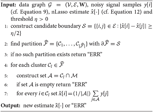
The noisy measurements y[i] are then input to an ADMM implementation for solving the nLasso problem (Equation 12) with λ = 1/K. We run ADMM for a fixed number of 300 iterations and using ADMM-parameter ρ = 0.01 [16]. In Figure 5 we illustrate the recovered graph signals (over the first 100 nodes of the chain graph) $\widehat{x}\left[·\right]$, obtained from noisy signal samples over either sampling set ${{M}}_1$ or ${{M}}_2$.

FIGURE 5

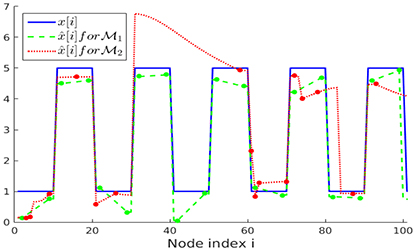
Figure 5. Clustered graph signal x[·] along with the recovered graph signals obtained from noisy signal samples set ${{M}}_1$ (Lemma 2) and ${{M}}_2$ (random).

As evident from Figure 5, the recovered signal obtained when using the sampling set ${{M}}_1$, which takes the partition ${{F}}_{\text{chain}}$ into account, better resembles the original graph signal x[·] than when using the randomly selected sampling set ${{M}}_2$. The favorable performance of ${{M}}_1$ is also reflected in the empirical normalized mean squared errors (NMSE) between the real and recovered graph signals, which are ${\text{NMSE}}_{{{M}}_1}=3.3·10^{-2}$ and ${\text{NMSE}}_{{{M}}_2}=2.192·10^{-1}$, respectively.

We have repeated the above experiment with the same parameters but considering noiseless initial samples y[i] for both sampling sets ${{M}}_1$ and ${{M}}_2$. The recovered graph signals $\widehat{x}\left[·\right]$ for the first 100 nodes of the chain are presented in Figure 6. It can be observed that the recovery starting from the sampling set ${{M}}_1$ (conforming to the partition ${{F}}_{\text{chain}}$) perfectly resembles the original graph signal x[·], as expected according to our upper bound in Equation (19). The NMSE obtained after running ADMM for 300 iterations for solving the nLasso problem (Equation 12) are ${\text{NMSE}}_{{{M}}_1}=7.5·10^{-6}$ and ${\text{NMSE}}_{{{M}}_2}=1.475·10^{-1}$, respectively.

FIGURE 6

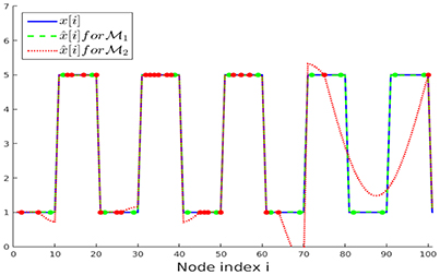
Figure 6. Clustered graph signal x[·] along with the recovered graph signals obtained from noiseless signal samples over sampling set ${{M}}_1$ (Lemma 2) and ${{M}}_2$ (random). The noiseless signal samples y[i] = x[i] are marked with dots.

4.2. Complex Network

In this second experiment, we generate a data graph ${{G}}_{\text{lfr}}$ using the generative model introduced by Lancichinetti et al. [40], in what follows referred to as LFR model. The LFR model aims at imitating some key characteristics of real-world networks such as power law distributions of node degrees and community sizes. The data graph ${{G}}_{\text{lfr}}$ contains a total of N = 10⁵ nodes which are partitioned into 1,399 clusters, ${{F}}_{\text{lfr}}=\left\{{{C}}_1,\dots ,{{C}}_{1399}\right\}$. The nodes ${V}$ of ${{G}}_{\text{lfr}}$ are connected by a total of 9.45·10⁵ undirected edges ${E}$.

The edge weights W_{i, j}, which are also provided by the LFR model, conform to the cluster structure of ${{G}}_{\text{lfr}}$, i.e., inter-cluster edges $\left\{i,j\right\}\in {E}$ with $i,j\in {{C}}_l$ have larger weights compared to intra-cluster edges $\left\{i,j\right\}\in {E}$ with $i\in {{C}}_l$ and $j\in {{C}}_{l^{\prime }}$. Given the data graph ${{G}}_{\text{lfr}}$ and partition ${{F}}_{\text{lfr}}$ we generate a clustered graph signal according to Equation (4) as $x\left[i\right]=\sum _{j=1}^{1399}{a}_j{{I}}_{{{C}}_j}\left[i\right]$ with coefficients a_j randomly chosen i.i.d. according to a uniform distribution ${U}(1,50)$.

We then try to recover the entire graph signal x[·] by solving the nLasso problem (Equation 12) using noisy measurements y[i], according to Equation (9) with i.i.d. measurement noise $e\left[i\right]~{N}(0,1/4)$, obtained at the nodes in a sampling set ${M}$. As in section 4.1, we consider two different choices ${{M}}_1$ and ${{M}}_2$ for the sampling set which both contain the same number of nodes, i.e., $\left|{{M}}_1\right|=\left|{{M}}_2\right|=10^4$. The nodes in sampling set ${{M}}_1$ are selected according to Lemma 2, i.e., by choosing nodes which are well connected (close) to boundary edges $\partial {{F}}_{\text{lfr}}$ which connect different clusters of the partition ${{F}}_{\text{lfr}}$. In contrast, the sampling set ${{M}}_2$ is constructed by selecting nodes uniformly at random, i.e., the partition ${{F}}_{\text{lfr}}$ is not taken into account.

In order to construct the sampling set ${{M}}_1$, we first sorted the edges $\left\{i,j\right\}\in {E}$ of the data graph ${{G}}_{\text{lfr}}$ in ascending order according to their edge weight W_{i, j}. We then iterate over the the edges according to the list, starting with the edge having smallest weight, and for each edge $\left\{i,j\right\}\in {E}$ we select the neighboring nodes of i and j with highest degree and add them to ${{M}}_1$, if they are not already included there. This process continues until the sampling set ${{M}}_1$ has reached the prescribed size of 10⁴. Using Lemma 2, we then verified numerically that the sampling set ${{M}}_1$ resolves ${{F}}_{\text{lfr}}$ with constants K = 142.6 and L = 2 (cf. Definition 1).

The measurements y[i] collected for each sampling sets ${{M}}_1$ and ${{M}}_2$ are fed into the ADMM algorithm (using parameters ρ = 1/100) for solving the nLasso problem (Equation 12) with λ = 1/K. The evolution of the NMSE achieved by the ADMM output for an increasing number the iterations is shown in Figure 7. According to Figure 7 the signal recovered from the sampling set ${{M}}_1$ approximates the true graph signal x[·] more closely compared to when using the sampling set ${{M}}_2$. The NMSE achieved after 300 iterations of ADMM is ${\text{NMSE}}_{{{M}}_1}=1.56·10^{-2}$ and ${\text{NMSE}}_{{{M}}_2}=4.25·10^{-2}$, respectively.

FIGURE 7

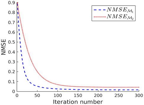
Figure 7. Evolution of the NMSE achieved by increasing number of nLasso-ADMM iterations when using sampling set ${{M}}_1$ or ${{M}}_2$, respectively.

Finally, we compare the recovery accuracy of nLasso to that of plain label propagation (LP) [41], which relies on a band-limited signal model (cf. section 2.1). In particular, LP quantifies signal smoothness by the Laplacian quadratic form (Equation 6) instead of the total variation (Equation 1), which underlies nLasso (Equation 12). The signals recovered after running the LP algorithm for 300 iterations for the two sampling sets ${{M}}_1$ and ${{M}}_2$ incur an NMSE of ${\text{NMSE}}_{{{M}}_1}=3.1·10^{-2}$ and ${\text{NMSE}}_{{{M}}_2}=7.43·10^{-2}$, respectively. Thus, the signals recovered using nLasso are more accurate compared to LP, as illustrated in Figure 8. However, our results indicate that LP also benefits by using the sampling set ${{M}}_1$ whose construction is guided by our theoretical findings (cf. Lemma 2).

FIGURE 8

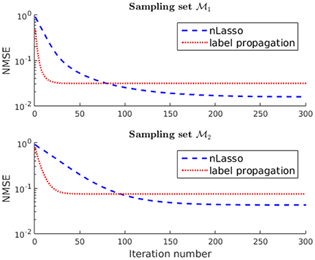
Figure 8. Evolution of the NMSE achieved by increasing number of nLasso-ADMM iterations and LP iterations. Both algorithms are fed with the same signal samples obtained either over sampling set ${{M}}_1$ or ${{M}}_2$, respectively.

5. Proofs

The high-level idea behind the proof of Theorem 3 is to adapt the concept of compatibility conditions for Lasso type estimators [32]. This concept has been championed for analyzing Lasso type methods [32]. Our main technical contribution is to verify the compatibility condition for a sampling set ${M}$ which resolves the partition ${F}$ underlying the signal model (Equation 4) (cf. Lemma 6 below).

5.1. The Network Compatibility Condition

As an intermediate step toward proving Theorem 3, we adopt the compatibility condition [42], which has been introduced to analyze Lasso methods for learning sparse signals, to the clustered graph signal model (Equation 4). In particular, we define the network compatibility condition for sampling graph signals with small total variation (cf. Equation 1).

Definition 5. Consider a data graph ${G}=({V},{E},\text{W})$ whose nodes ${V}$ are partitioned into disjoint clusters ${F}=\left\{{{C}}_1,\dots ,{{C}}_{\left|{F}\right|}\right\}$. A sampling set ${M}\subseteq {V}$ is said to satisfy the network compatibility condition, with constants K, L > 0, if

$\begin{array}{ll}K{\displaystyle \sum _{i\in {M}}|}z[i]|+\Vert z[·]{\Vert }_{{E}\setminus \partial {F}}\ge L\Vert z[·]{\Vert }_{\partial {F}}& (22)\end{array}$

for any graph signal $z\left[·\right]\in {ℝ}^{{V}}$.

It turns out that any sampling set ${M}$ which resolves the partition ${F}=\left\{{{C}}_1,\dots ,{{C}}_{\left|{F}\right|}\right\}$ with constants K and L (cf. Definition 1) also satisfies the network compatibility condition (Equation 22) with the same constants.

Lemma 6. Any sampling set ${M}$ which resolves the partition ${F}$ with parameters K, L > 0 satisfies the network compatibility condition with parameters K, L.

Proof: Let us consider an arbitrary but fixed graph signal $z\left[·\right]\in {ℝ}^{{V}}$. Since the sampling set ${M}$ resolves the partition ${F}$ there exists a flow h[e] on ${G}$ with (cf. Definition 1)

$\begin{array}{l}{\displaystyle \sum _{j\in {N}(i)}h}(j,i)-{\displaystyle \sum _{j\in {N}(i)}h}(i,j)=0\text{for all }i\notin {M}\\ {\displaystyle |{\displaystyle \sum _{j\in {N}(i)}h}(j,i)-{\displaystyle \sum _{j\in {N}(i)}h}(i,j)|}\le K\text{for all}i\in {M}\\ |h(i,j)|\le W_{i,j}\text{for}(i,j)\notin \partial {F}\\ h(i,j)·h(j,i)=0\text{for}\{i,j\}\in \partial {F}& (23)\end{array}$

Moreover, due to Equation (15), we have the important identity

$\begin{array}{ll}(h(i,j)-h(j,i))(z[i]-z[j])=L{W}_{i,j}|z[i]-z[j]|& (24)\end{array}$

which holds for all boundary edges $\left\{i,j\right\}\in \partial {F}$. This yields, in turn,

$\begin{array}{l}L\Vert z[·]{\Vert }_{\partial {F}}\stackrel{(2)}{=}{\displaystyle \sum _{\{i,j\}\in \partial {F}}|}z[i]-z[j]|L{W}_{i,j}\\ \stackrel{(24)}{=}{\displaystyle \sum _{(i,j)\in \partial {F}}(z[i]-z[j])}h(i,j).& (25)\end{array}$

Since ${E}$ = ∂${F}$∪(${E}$\∂${F}$), we can develop (Equation 25) as

$\begin{array}{l}L\Vert z[·]{\Vert }_{\partial {F}}\\ ={\displaystyle \sum _{(i,j)\in {E}}(z[i]-z[j])h(i,j)}-{\displaystyle \sum _{(i,j)\in {E}\setminus \partial {F}}(z[i]-z[j])h(i,j)}\\ ={\displaystyle \sum _{i\in {V}}z}[i]{\displaystyle \sum _{j\in {N}(i)}(h(j,i)-h(i,j))}\\ -{\displaystyle \sum _{(i,j)\in {E}\setminus \partial {F}}(z[i]-z[j])h(i,j)}\\ \stackrel{(23)}{\le }K{\displaystyle \sum _{i\in {M}}|}z[i]|+{\displaystyle \sum _{\{i,j\}\in {E}\setminus \partial {F}}|}z[i]-z[j]|W_{i,j}\\ =K{\displaystyle \sum _{i\in {M}}|}z[i]|+\Vert z[·]{\Vert }_{{E}\setminus \partial {F}}& (26)\end{array}$

which verifies (Equation 22).    □

The next result shows that if the sampling set satisfies the network compatibility condition, any solution of the nLasso (Equation 12) allows to accurately recover a clustered graph signal (cf. Equation 4).

Lemma 7. Consider a clustered graph signal x[·] of the form (Equation 4) defined on the data graph ${G}=({V},{E},\text{W})$ whose nodes ${V}$ are partitioned into the clusters ${F}=\left\{{{C}}_1,\dots ,{{C}}_{\left|{F}\right|}\right\}$. We observe the noisy signal values y[i] at the sampled nodes ${M}\subseteq {V}$ (cf. Equation 9). If the sampling set ${M}$ satisfies the network compatibility condition with constants L > 1, K > 0, then any solution of the nLasso problem (Equation 12), for the choice λ: = 1/K, satisfies

$\begin{array}{ll}\Vert \widehat{x}[·]-x[·]{\Vert }_{\text{TV}}\le (K+4/(L-1)){\displaystyle \sum _{i\in {M}}|}e[i]|.& (27)\end{array}$

Proof: Consider a solution $\widehat{x}\left[·\right]$ of the nLasso problem (Equation 12) which is different from the true underlying clustered signal x[·] (cf. Equation 4). We must have (cf. Equation 9)

$\begin{array}{ll}{\displaystyle \sum _{i\in {M}}|\widehat{x}[i]-y[i]|}+\lambda \Vert \widehat{x}[·]{\Vert }_{\text{TV}}\le {\displaystyle \sum _{i\in {M}}|e[i]|}+\lambda \Vert x[·]{\Vert }_{\text{TV}}& (28)\end{array}$

since otherwise the true underlying signal x[·] would achieve a smaller objective value in Equation (12) which, in turn, would contradict the premise that $\widehat{x}\left[·\right]$ is optimal for the problem (Equation 12).

Let us denote the difference between the solution $\widehat{x}\left[·\right]$ of Equation (12) and the true underlying clustered signal x[·] by $\tilde{x}\left[·\right]:=\widehat{x}\left[·\right]-x\left[·\right]$. Since x[·] satisfies Equation (4),

$\begin{array}{ll}\Vert x[·]{\Vert }_{{E}\setminus \partial {F}}=0,\text{ and }\Vert \tilde{x}[·]{\Vert }_{{E}\setminus \partial {F}}=\Vert \widehat{x}[·]{\Vert }_{{E}\setminus \partial {F}}.& (29)\end{array}$

Applying the decomposition property of the semi-norm || · ||_TV to Equation (28) yields

$\begin{array}{l}{\displaystyle \sum _{i\in {M}}|\widehat{x}[i]-y[i]|+\lambda \Vert \widehat{x}[·]{\Vert }_{{E}\setminus \partial {F}}}\\ \le {\displaystyle \sum _{i\in {M}}|}e[i]|+\lambda \Vert x[·]{\Vert }_{\partial {F}}-\lambda \Vert \widehat{x}[·]{\Vert }_{\partial {F}}.& (30)\end{array}$

Therefore, using Equation (29) and the triangle inequality,

$\begin{array}{l}{\displaystyle \sum _{i\in {M}}|}\widehat{x}[i]-y[i]|+\lambda \Vert \tilde{x}[·]{\Vert }_{{E}\setminus \partial {F}}\\ \le \lambda \Vert \tilde{x}[·]{\Vert }_{\partial {F}}+{\displaystyle \sum _{i\in {M}}|}e[i]|.& (31)\end{array}$

Since $\sum _{i\in {M}}|\widehat{x}\left[i\right]-y\left[i\right]|\ge 0$, Equation (31) yields

$\begin{array}{ll}\lambda \Vert \tilde{x}[·]{\Vert }_{{E}\setminus \partial {F}}\le \lambda \Vert \tilde{x}[·]{\Vert }_{\partial {F}}+{\displaystyle \sum _{i\in {M}}|}e[i]|,& (32)\end{array}$

i.e., for sufficiently small measurement noise e[i], the signal differences of the recovery error $\tilde{x}\left[·\right]=\widehat{x}\left[·\right]-x\left[·\right]$ cannot be concentrated across the edges within the clusters ${{C}}_l$. Moreover, using

$\begin{array}{l}{\displaystyle \sum _{i\in {M}}|}\widehat{x}[i]-y[i]|\stackrel{(9)}{=}{\displaystyle \sum _{i\in {M}}|}\widehat{x}[i]-x[i]-e[i]|\\ \ge {\displaystyle \sum _{i\in {M}}|}\tilde{x}[i]|-{\displaystyle \sum _{i\in {M}}|}e[i]|,& (33)\end{array}$

the inequality Equation (31) becomes

$\begin{array}{ll}{\displaystyle \sum _{i\in {M}}|}\tilde{x}[i]|+\lambda \Vert \tilde{x}[·]{\Vert }_{{E}\setminus \partial {F}}\le \lambda \Vert \tilde{x}[·]{\Vert }_{\partial {F}}+2{\displaystyle \sum _{i\in {M}}|}e[i]|.& (34)\end{array}$

Thus, since the sampling set ${M}$ satisfies the network compatibility condition, we can apply Equation (22) to $\tilde{\text{x}}\left[·\right]$ yielding

$\begin{array}{ll}{\displaystyle \sum _{i\in {M}}|}\tilde{x}[i]|+(1/K)\Vert \tilde{x}[·]{\Vert }_{{E}\setminus \partial {F}}\ge (1/K)L\Vert \tilde{x}[·]{\Vert }_{\partial {F}}.& (35)\end{array}$

Inserting Equation (35) into Equation (34), with λ = 1/K, yields

$\begin{array}{ll}\lambda (L-1)\Vert \tilde{x}[·]{\Vert }_{\partial {F}}\le 2{\displaystyle \sum _{i\in {M}}|}e[i]|.& (36)\end{array}$

Combining Equations (32) and (36) yields

$\begin{array}{l}\Vert \tilde{x}[·]{\Vert }_{\text{TV}}=\Vert \tilde{x}[·]{\Vert }_{{E}\setminus \partial {F}}+\Vert \tilde{x}[·]{\Vert }_{\partial {F}}\\ \stackrel{(32)}{\le }2\Vert \tilde{x}[·]{\Vert }_{\partial {F}}+(1/\lambda ){\displaystyle \sum _{i\in {M}}|}e[i]|\\ \stackrel{(36)}{\le }\frac{1+4\lambda /(L-1)}{\lambda }{\displaystyle \sum _{i\in {M}}|e[i]|}.& (37)\end{array}$

  □

5.2. Proof of Theorem 3

Combine Lemma 6 with Lemma 7.

6. Conclusions

Given a known cluster structure of the data graph, we introduced the notion of resolving sampling sets. A sampling set resolves a cluster structure if there exists a sufficiently large network flow between the sampled nodes, with prescribed flow values over boundary edges which connect different clusters. Loosely speaking, this requires to choose the sampling set mainly in the boundary regions between different clusters in the data graph. Thus, we can leverage efficient clustering methods for identifying the cluster boundary regions in order to find sampling sets which resolve the intrinsic cluster structure of the network structure underlying a dataset.

The verification if a particular sampling set resolves a given partition requires to consider all possible sign patterns for the boundary edges, which is intractable for large graphs. An important avenue for follow-up work is the investigation if resolving sampling sets can be characterized easily using probabilistic models for the underlying network structure and sampling sets. Moreover, we plan to extend our analysis to nLasso methods using other loss functions, e.g., the squared error loss and also the logistic loss function in the context of classification problems.

Author Note

Parts of the work underlying this paper have been presented in Mara and Jung [43]. A preprint of this manuscript is available under https://arxiv.org/abs/1704.02107 [44].

Author Contributions

AJ initiated the research and provided first proofs for the main results. NT helped with proof reading and pointing to some typos in the proofs. AM took care of the numerical experiments.

Conflict of Interest Statement

The authors declare that the research was conducted in the absence of any commercial or financial relationships that could be construed as a potential conflict of interest.

Acknowledgments

The authors are grateful to Madelon Hulsebos for a careful proof-reading of an early manuscript. Moreover, the constructive comments of reviewers are appreciated sincerely. This manuscript is available as a pre-print at the following address: https://arxiv.org/abs/1704.02107. Copyright of this pre-print version rests with the authors.

References

1. Sandryhaila A, Moura JMF. Classification via regularization on graphs. In 2013 IEEE Global Conference on Signal and Information Processing. Austin, TX (2013). p. 495–8. doi: 10.1109/GlobalSIP.2013.6736923

CrossRef Full Text | Google Scholar

2. Chen S, Sandryhaila A, Moura JMF, Kovačević J. Signal recovery on graphs: variation minimization. IEEE Trans Signal Process. (2015) 63:4609–24. doi: 10.1109/TSP.2015.2441042

CrossRef Full Text | Google Scholar

3. Bishop CM. Pattern Recognition and Machine Learning. New York, NY: Springer (2006).

Google Scholar

4. Chapelle O, Schölkopf B, Zien A, (eds.). Semi-Supervised Learning. Cambridge, MA: The MIT Press (2006). doi: 10.7551/mitpress/9780262033589.001.0001

CrossRef Full Text | Google Scholar

5. Zhou D, Schölkopf B. A regularization framework for learning from graph data. In: ICML Workshop on Statistical Relational Learning and Its Connections to Other Fields, vol. 15. Banff (2004). p. 67–8.

Google Scholar

6. Gadde A, Anis A, Ortega A. Active semi-supervised learning using sampling theory for graph signals. In: Proceedings of the 20th ACM SIGKDD International Conference on Knowledge Discovery and Data Mining. KDD '14 (2014). p. 492–501. doi: 10.1145/2623330.2623760

CrossRef Full Text | Google Scholar

7. Ando RK, Zhang T. Learning on graph with laplacian regularization. In: Advances in Neural Information Processing Systems. Vancouver, BC (2007).

Google Scholar

8. Belkin M, Niyogi P, Sindhwani V. Manifold regularization: a geometric framework for learning from labeled and unlabeled examples. J Mach Lear Res. (2006) 7:2399–434.

Google Scholar

9. Sandryhaila A, Moura JMF. Big data analysis with signal processing on graphs: representation and processing of massive data sets with irregular structure. IEEE Signal Process Mag. (2014) 31:80–90. doi: 10.1109/MSP.2014.2329213

CrossRef Full Text | Google Scholar

10. Shuman DI, Narang SK, Frossard P, Ortega A, Vandergheynst P. The emerging field of signal processing on graphs: extending high-dimensional data analysis to networks and other irregular domains. IEEE Signal Process Mag. (2013) 30:83–98. doi: 10.1109/MSP.2012.2235192

CrossRef Full Text

11. Narang SK, Gadde A, Ortega A. Signal processing techniques for interpolation in graph structured data. In: 2013 IEEE International Conference on Acoustics, Speech and Signal Processing (2013). p. 5445–9. doi: 10.1109/ICASSP.2013.6638704

CrossRef Full Text

12. Hallac D, Leskovec J, Boyd S. Network Lasso: clustering and optimization in large graphs. In: Proceedings of SIGKDD (2015). p. 387–96. doi: 10.1145/2783258.2783313

CrossRef Full Text

13. Hastie T, Tibshirani R, Friedman J. The Elements of Statistical Learning. Springer Series in Statistics. New York, NY: Springer (2001).

14. Hastie T, Tibshirani R, Wainwright M. Statistical Learning with Sparsity. The Lasso and its Generalizations. Boca Raton FL: CRC Press (2015).

15. Yamada M, Koh T, Iwata T, Shawe-Taylor J, Kaski S. Localized lasso for high-dimensional regression. In: Proceedings of the 20th International Conference on Artificial Intelligence and Statistics. Fort Laud-erdale, FL (2017). p. 325–33.

16. Boyd S, Parikh N, Chu E, Peleato B, Eckstein J. Distributed Optimization and Statistical Learning via the Alternating Direction Method of Multipliers. vol. 3 of Foundations and Trends in Machine Learning. Hanover, MA: Now Publishers (2010).

17. Romero D, Ma M, Giannakis GB. Kernel-based reconstruction of graph signals. IEEE Trans Signal Process. (2017) 65:764–78. doi: 10.1109/TSP.2016.2620116

CrossRef Full Text

18. Tsitsvero M, Barbarossa S, Lorenzo PD. Signals on graphs: uncertainty principle and sampling. IEEE Trans Signal Process. (2016) 64:4845–60. doi: 10.1109/TSP.2016.2573748

CrossRef Full Text

19. Chen S, Varma R, Sandryhaila A, Kovačević J. Discrete signal processing on graphs: sampling theory. IEEE Trans Signal Process. (2015) 63:6510–23. doi: 10.1109/TSP.2015.2469645

CrossRef Full Text

20. Chen S, Varma R, Singh A, Kovačević J. Signal recovery on graphs: fundamental limits of sampling strategies. IEEE Trans Signal Inform Process Over Netw. (2016) 2:539–54. doi: 10.1109/TSIPN.2016.2614903

CrossRef Full Text

21. Segarra S, Marques AG, Leus G, Ribeiro A. Reconstruction of graph signals through percolation from seeding nodes. IEEE Trans Signal Process. (2016) 64:4363–78. doi: 10.1109/TSP.2016.2552510

CrossRef Full Text

22. Wang X, Liu P, Gu Y. Local-set-based graph signal reconstruction. IEEE Trans Signal Process. (2015) 63:2432–44. doi: 10.1109/TSP.2015.2411217

CrossRef Full Text

23. Sharpnack J, Rinaldo A, Singh A. Sparsistency of the Edge Lasso over Graphs. AIStats (JMLR WCP). La Palma (2012).

24. Wang YX, Sharpnack J, Smola AJ, Tibshirani RJ. Trend filtering on graphs. J Mach Lear Res. (2016) 17:1–41. Available online at: http://jmlr.org/papers/v17/15-147.html

25. Golub GH, Van Loan CF. Matrix Computations. 3rd Edn. Baltimore, MD: Johns Hopkins University Press (1996).

26. Goodfellow I, Bengio Y, Courville A. Deep Learning. Cambridge, MA: MIT Press (2016).

27. Cui S, Hero A, Luo ZQ, Moura JMF, (eds.). Big Data Over Networks. Cambridge, UK: Cambridge University Press (2016).

28. Zhu X, Rabbat M. Graph spectral compressed sensing for sensor networks. In: Proceedings of IEEE ICASSP 2012. Kyoto (2012). p. 2865–8.

29. Newman MEJ. Networks: An Introduction. New York, NY: Oxford University Press (2010).

30. Mossel E, Neeman J, Sly A. Stochastic block models and reconstruction. ArXiv e-prints. (2012).

31. Bapat RB. Graphs and Matrices. London: Springer-Verlag (2014).

32. Bühlmann P, van de Geer S. Statistics for High-Dimensional Data. New York, NY: Springer (2011).

33. Chambolle A, Pock T. An introduction to continuous optimization for imaging. Acta Numer. (2016) 25:161–319. doi: 10.1017/S096249291600009X

CrossRef Full Text

34. Agarwal A, Negahban S, Wainwright MJ. Fast global convergence of gradient methods for high-dimensional statistical recovery. Ann Stat. (2012) 40:2452–82. doi: 10.1214/12-AOS1032

CrossRef Full Text

35. Boyd S, Vandenberghe L. Convex Optimization. Cambridge: Cambridge University Press (2004).

36. Zhu Y. An augmented ADMM algorithm with application to the generalized lasso problem. J Comput Graph Stat. (2017) 26:195–204. doi: 10.1080/10618600.2015.1114491

CrossRef Full Text

37. Kleinberg J, Tardos E. Algorithm Design. New York, NY: Addison Wesley (2006).

38. Spielman DA, hua Teng S. A local clustering algorithm for massive graphs and its application to nearly-linear time graph partitioning. arXiv:0809.3232 (2008).

39. Basirian S, Jung A. Random walk sampling for big data over networks. In: Proceedings of International Conference on Sampling Theory and Applications. Tallinn (2017).

40. Lancichinetti A, Fortunato S, Radicchi F. Benchmark graphs for testing community detection algorithms. Phys Rev E (2008) 78:046110. doi: 10.1103/PhysRevE.78.046110

CrossRef Full Text

41. Zhu X, Ghahramani Z. Learning from Labeled and Unlabeled Data with Label Propagation. Technical Report CMU-CALD-02-107, Carnegie Mellon University (2002).

42. van de Geer SA, Bühlmann P. On the conditions used to prove oracle results for the Lasso. Electron J Stat. (2009) 3:1360–92. doi: 10.1214/09-EJS506

CrossRef Full Text

43. Mara A, Jung A. Recovery conditions and sampling strategies for network lasso. In: Proceedings of 51st Asilomar Conference Signals, Systems, Computers. Pacific Grove, CA (2017).

44. Jung A, Tran NQ, Mara A. When is network lasso accurate? arXiv:170402107 (2017).