Predicting Dynamical Crime Distribution From Environmental and Social Influences

Introduction

Recent advances in the spatial analysis of crime strongly affected the ways in which scholars and practitioners consider the origins and dispersion of crime. Hotspot mapping [1] and near repeat analysis [2] have allowed police to more efficiently target criminogenic places. Analyses of the physical contexts for crime was pioneered in criminology by Brantingham and Brantingham [3], who considered the underlying social and physical “fabric” or environmental backcloth as a framework for action. More recently, Caplan and Kennedy [4] proposed Risk Terrain Modeling (RTM) as a spatial analytical technique for empirical study of crime distribution. Resulting risk terrain maps show where certain crime events are statistically more likely to occur based on certain environmental vulnerabilities at micro places [4–7]. This technique considers the effects of multiple factors on creating distinct, identifiable areas that are conducive to crime, but emphasizes the importance of environmental characteristics on the attraction of motivated offenders and the emergence, persistence, and desistance of crime [4–6]. For each place, it produces a risk score, that is a measure of the clustering of environmental risk factors, and can be used to forecast where crime will occur and (possibly) cluster over a period of time.

Spatial analysis—as it is used in the criminological research literature—often ignores the mechanism through which disconnected offenders cluster in space and time despite a seeming lack of deliberate coordination of activities. For instance, Sherman et al. [1] found that up to 50% of crime is produced at 3% of city locations. While Spelman [8] concluded that the statistical concentration of crime at places may be due to random and often temporary fluctuations in crime events, [9] noted that, even after correcting for such fluctuations, the worst locations accounted for a disproportionately high number of crime incidents. It appears as though, through independent action, offenders ultimately converge at the same places over given periods of time to commit similar types of crimes. If this is the case, why is this so, and how do offenders know where to go?

A possible answer comes from the concept of near repeat victimization that states that a criminal incident increases the likelihood that a nearby location or individual will be targeted in a subsequent incident [10]. This can result from either the same perpetrator repeating a crime in a location where it has been successful, or from new perpetrators encouraged directly (e.g., by a member of the same gang) or indirectly (e.g., by traces indicative of a successful event) by the first one. This has the potential of creating a positive feedback loop, with subsequent criminal events in what are defined as risky places—if close enough in space and time - increasing further the probability of additional events clustering in the same area, and so on Kennedy et al. [11]. This is described in the Theory of Risky Places [12], where the vulnerability that comes from being in high risk locations, combined with the exposure to offenders, leads to a greater probability of crime occuring.

While this concept is fairly recent in criminology, it is well-known in the scientific literature on collective behavior in biological systems. Similar feedback loops driven by past events and social information have been found to create clustering in unicellular organisms, insects, fish, birds, and mammals [13–15], even in uniform environmental conditions. However the final location of the cluster is highly dependent on the structure of the environment: clusters are more likely to originate at attractive places for the organisms, and the positive feedback process will promote the disproportionate concentration of individuals at some of the attracting places only (sometimes at a single one) while others will be abandoned [13, 16–18]. In addition, once this process has reached its stable state, the probability of starting a new cluster elsewhere—even at another attractive location - is low [13].

The striking parallel between the mechanisms of crime hotspot formation and those of clustering in social animals suggests that crime suppression and prevention efforts would strongly benefit from better understanding the combined effects of the social and physical environments in which offenders operate. For this purpose, we propose here to combine tools for the spatial analysis of crime with methods for measuring and modeling social influence in animal groups, with the goal of improving methods for forecasting crime distribution. In particular we will use RTM as a tried and tested method to identify environmental predictors of criminal events; we will also use simulation methods to determine spatio-temporal correlations between successive events, after controlling for environmental effects. Finally, we will show that combining event-dependent and environmental influences provides improvement in forecasting changes in crime distribution over purely spatial methods (e.g., RTM) or methods based on modeling near repeat victimization only.

Materials and Methods

Data

Crime Data

This study selectively focuses on street robberies, or robberies that occur at outdoor public spaces (e.g., streets, sidewalks, parking lots, lots/yards in front of commercial dwellings) between 2009 and 2012 in Newark, New Jersey (6,888 recorded events). The robbery data were acquired from the public records of the Newark Police Department (NPD). They only contain the time, location and nature of criminal offenses without identifying information on either the perpetrators or their victims, and therefore an ethics approval was not required as per institutional and national guidelines. Adopting the FBI's UCR Part I crime definitions, the NPD defines robbery as “the taking or attempting to take anything from the care, custody, or control of a person or persons by force or threat of force or violence and/or by putting the victim in fear” [19]. The robbery dataset includes each incident's longitude and latitude coordinates, as well as the date (e.g., 07.28.2010), day (e.g., Monday or Saturday), and hour (0–23. where 0 denotes 12 a.m.) of occurrence. For the analyses, Newark was modeled as a contiguous grid of equally sized cells the length of about half a city block (the mean blockface length is approximately 137.77 m). Each incident was therefore associated with the 68.88 m by 68.88 m cell containing its longitude and latitude coordinates.

Land Use Data

The independent variables (risk factors) of the risk terrain model were the operationalized spatial influences of land use features in Newark; the following 20 criminogenic features were included for testing in the RTM analysis: packaged liquor stores, take-out restaurants, gas stations, college campuses, parks, convenience stores, light rail stops, eat-in restaurants, foreclosed properties, parking garages, pawn shops, gyms and health clubs, grocery stores, recreation centers, at-risk housing, vacant properties, laundromats, bars, known drug markets, and schools. These data were acquired from the NPD Compstat unit or from InfoGroup, a lead provider of verified business data in the U.S.

All land use data coordinates were converted to cell coordinates matching the spatial coordinates of the crime data.

Risk Terrain Map

A risk terrain map represents the risk of a criminal event occurring at a location given the land use features of this location (see section Land Use Data above for a list of the land use features tested in this study) and relative to all the other locations considered in the analysis (all cells have approximately the size of half city blocks in Newark in this study). RTM is used to identify the relative influence of each land use feature on the occurrence of criminal events and these influences are then combined to calculate the overall relative risk associated with each considered location.

RTM has been described in detail elsewhere [6] and we will only describe its general functioning here. RTM is a two-step modeling process. In the first step RTM uses an elastic net penalization from the “penalized” R package [20] with cross-validation to perform both variable selection and regularization on a Poisson regression model of environmental risks. Model factors that stand up to shrinkage with nonzero coefficients in the penalized model are accepted as useful risk factors and passed to the next step for building the most parsimonious model.

In the second step RTM conducts a bidirectional stepwise regression using the “gamlss” R package [21] on the remaining risk factors resulting from the first step. Stepwise regression is a method to automatically reduce the complexity of a statistical model by identifying the predictive variables that significantly improve the fit to the data. The process consists in adding and removing predictive variables in a stepwise manner (i.e., one predictor at a time) and evaluating whether it significantly improves the fit to the data using in our case a BIC (Bayesian Information Criterion) score. The BIC score is a measure of the likelihood of the fit penalized by the number of predictors in the model. The model with the lowest BIC score is preferred as it strikes a balance between higher likelihood of the fit and lower complexity of the model. We repeated this process twice: once assuming a Poisson distribution of the model's residuals, and another time assuming a negative binomial distribution. Overall relative risk scores are then produced for each cell unit to produce the final risk terrain map covering the entire geographic extent of the Newark study area, which excluded the seaport and airport areas because their crimes fall under a different law enforcement jurisdiction than the NPD.

For the current study, the risk terrain map was produced using the RTMDx software, which was developed by Rutgers Center on Public Security [5]. This utility automates the RTM steps of operationalizing the spatial influence of risk factors, selecting/validating the risk factors with existing outcome event data, weighting the risk factors in relation to one another, and producing the final risk terrain map.

For each of the 20 potential risk factors described in section Land Use Data, at least 6 variables were built to measure spatial influences. These measured whether the raster cells in Newark were within 0.5, 1, 1.5, 2, 2.5, or 3 blocks of the features or in an area of high density of the factor's features. Although the extent of spatial influence can theoretically be operationalized at less than one-half block or beyond three blocks, these distances were set as the minimum and maximum search extents because they are believed to give a meaningful reach of a land use feature's influence from a policing perspective [22, 23], and the half-block increments were used to account for varying extents of the land use features' spatial influences. For both the distance and the density calculations, we determined which cells of the study area fall into the areas defined by the different spatial extents by calculating the distance of the cell centroids to the land use feature of interest ([24], p. 5). Then, raster cells that fall within the threshold proximity (0.5, 1, 1.5, 2, 2.5, or 3 blocks) were represented as 1 (highest risk), whereas the cells outside this threshold proximity were represented as 0 (not highest risk). Density variables were reclassified into highest density (density ≥ mean + 2 standard deviations) and not highest density (density < mean + 2 standard deviations) regions. Highest density regions were represented as 1, and regions that are not highest density were represented as 0. Ultimately, 186 model factors were produced that represent various distances from or densities of the 20 land use features in the risk terrain model. These values were then assembled into a table with rows representing cells and columns representing binary variables, and the count of street robbery events (the dependent variable) at each raster cell was calculated.

Spatio-Temporal Event-Dependence

The near repeat victimization hypothesis states that the occurrence of a criminal event at a location increases the likelihood of a subsequent event occurring at the same or a nearby location within a given time window. In order to measure this effect, we first calculate the spatio-temporal association between events as follows. For each robbery event in Newark in 2009 and 2010 we compute the probability that another event occurred within m cells from (m = 0, 1, 2, …, 40) and n days after (n = 0, 1, 2, …, 40) the original event.

The next step is to determine whether these probabilities are higher/lower than those expected under the assumption that there are no spatio-temporal dependence between events. For this, we use a permutation method to generate 1,000 surrogate data sets (of the same length as the original data set) in which the dependence between successive events is broken. First we randomly sample crime locations from the original data set with replacement. The probability of sampling a given location is proportional to the environmental risk value for this location as obtained from the RTM calculation (see previous section). We then associate a time to each surrogate location by randomly sampling existing occurrence times from the original data set with replacement. This procedure ensures that all surrogate events are independent in time, and that their spatial dependence is only driven by the structure of the environment, and not the location of previous events.

For each of the 1,000 surrogate data sets, we then calculate the spatio-temporal association between events following the same procedure as for the original data set. We then calculate the average ratio between the spatio-temporal association matrix of the original data set and that of the 1,000 surrogate data sets (a 2D Gaussian smoothing with standard deviation of 1 day and 1 cell is also applied to the resulting matrix). A ratio superior to 1 for a given combination of n and m indicates a likelihood higher than random for an event to occur m cells from and n days after a previous event. A ratio inferior to 1 indicates the opposite.

If the near repeat victimization hypothesis is correct, we expect to see a maximum increase in likelihood at m = 0 and n = 0, with a progressive decrease as both m and n increase.

Forecasting Model

We propose to integrate together the environmental influences determined via RTM and the event-dependent spatio-temporal associations determined via permutation in a computer simulation model. The goal of the model is to forecast the most likely locations of future crime occurrences, given a risk terrain map locally weighted by the presence of past crime occurrences. The general functioning of the model is as follows:

1. Calculate a risk terrain map of the area of interest as described in section Risk Terrain Map. This map will be fixed for the entirety of the simulation as we assume that environmental risks do not change faster than the time scale of the simulation (a few days to a few weeks in the case of this study).

2. Calculate the spatio-temporal influence of crime occurrences on future events as described in section Spatio-Temporal Event-Dependence.

3. Create an initial spatio-temporal event-dependent risk map using existing crime occurrence data. This map should have the same dimensions as the risk terrain map. All cells of the map are initially set to 1. Each cell's value is then modified according to the distance to and time since each past crime occurrence, based on the spatio-temporal influence ratio calculated in the previous step. We assume that the respective influences of multiple past events are additive.

4. For each simulation step (1 day in the case of this study),

a. determine the number of crime occurrences based on a distribution calculated from the original data set.

b. For each simulated crime occurrence:

i. Determine its location by randomly selecting a cell on the map. The probability of a cell being selected is proportional to the environmental risk value at its location on the risk terrain map multiplied by the event-dependent risk value at its location on the map.

ii. Update the event-dependent spatio-temporal risk map to include the influence of the new simulated event.

c. Before starting the next step, update the event-dependent spatio-temporal risk map to account for the temporal change in event-dependent spatial influence.

By simulating the model N times, we can compute a predicted probability of crime occurrence for each cell of the map.

Model Performance

We compare the forecasting performance of our model (referred to as full model in the rest of the text) against three control simulation models:

1. A random model, in which the locations of the simulated events will be selected independently of any environmental or event-dependent influence.

2. An environmental model only (referred to as RTM-only model in the rest of the text), in which the probability of a cell being selected is proportional to the environmental risk score at its location on the risk terrain map only.

3. An event-dependent spatio-temporal model only (referred to as event-only model in the rest of the text), in which the probability of a cell being selected is proportional to the the event risk value at its location on the event-dependent risk map only. Note that in this case, we will recompute the shape of the spatio-temporal influence as in section Spatio-Temporal Event-Dependence, but in absence of environmental influence.

For this comparison, we use a risk terrain map computed as described in section Risk Terrain Map using the Newark data from 2009 and 2010. The shape of the spatio-temporal influence is also computed using the 2009–2010 data. The data from 2011 and 2012 are used to initialize the event risk map and measure the performance of the models. This ensures that the model is never tested against data that has been used to parameterized it. In particular, each simulation starts at a given date in 2012 and the corresponding event risk map is initialized with all the data earlier than this date up to one year in the past.

Given a starting date, each model is simulated N times for n days after the starting date. For each actual crime occurrence in the n days after the start date, we compute the proportion ρ of simulated events that fall within 5 blocks of it. A higher average value of ρ indicates a higher clustering of simulated events around real events and therefore a better ability of the model to forecast changes in crime distribution. We can then rank the models by measuring the ratio between their average ρ and the average ρ of the random model which does not have any predictive ability.

Results

Risk Terrain Map

According to the results of the bidirectional stepwise regression presented in Table 1, the risk terrain exhibits 11 land use features that have a criminogenic spatial influence on robberies in Newark (see Table 1). The Relative Risk Values in the table correspond to the exponentiated coefficients for each predictive variable in the best model selected by the RTM procedure. Once exponentiated, each coefficient is the multiplier value corresponding to a unit change in the respective predictive variable. They convey the weighting of the variables in relation to one another and reveals that a single feature might be a more or less important factor for the emergence of robberies at particular places. For instance, places influenced by nearby gas stations are almost twice as risky, or vulnerable, to robbery as places influenced by nearby takeout restaurants.

TABLE 1

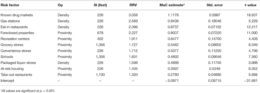
Table 1. Negative binomial type II Risk Terrain Model Factors: MuC, mean parameter coefficients; standard errors; RRV, relative risk values; Op, operationalizations; SI, spatial influence.

Places that are under the combined criminogenic spatial influence of these land use features had a higher risk of robberies than the places that were not. The risk terrain map represents weighted combinations of these risks at places throughout Newark, with risk scores ranging from the minimum standardized risk score of 1 to the maximum of 249.059 (see Figure 1A). So a place with a risk score of 249 had an expected rate of robberies that is 249 times higher than a place with a risk score of 1.

FIGURE 1

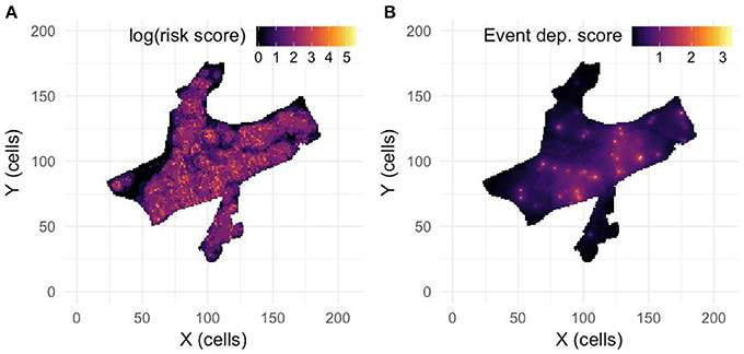
Figure 1. (A) Risk terrain map calculated for robberies in Newark using data from January 1, 2009 to December 31, 2010 following the method described in section Risk Terrain Map. Lighter colors indicate cells with higher relative risk values (log scale). (B) Event dependence map calculated using data from January 1, 2011 to December 31, 2011 and Equation 1. Lighter colors indicate cells with elevated risk due to past robbery occurrences.

Spatio-Temporal Event-Dependence

In the 2009–2010 data, the distribution of the number of daily robbery occurrences follows a Poisson distribution with an average value of λ ≃ 3.97 (see Figure S1A) and we observe no strong autocorrelation between successive days (see Figure S1B). In the model, we use this Poisson distribution without autocorrelation to randomly allocate a number of crime occurrences to each time step of the simulation.

As expected under the near repeat victimization hypothesis, we observe a maximum increase in likelihood (3.59) at m = 0 cells and n = 0 days, with a progressive decrease as both m and n increase (see Figure 2). We find that this likelihood landscape can be well approximated by an inverse function of m combined with a decreasing exponential function of n, of the form:

$\begin{array}{cc}1+\frac{\alpha e^{\delta n}}{\beta m+\gamma }& (1)\end{array}$

with α ≃ 2.59, β ≃ 1.47, γ = 1 and δ ≃ −0.32 when environmental influences are taken into account during the permutation process, and with α ≃ 4.62, β ≃ 1.1, γ = 1 and δ ≃ −0.2 when they are not.

FIGURE 2

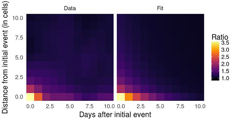
Figure 2. Spatio-temporal influence of previous robbery occurrences on future events calculated with data from January 1, 2009 to December 31, 2010 following the method described in section Spatio-Temporal Event-Dependence (Left), and its fit with Equation 1 (Right). The colors represent the ratio between the probability that another event occurred within m cells from and n days after the original event and the same probability after random permutation of the events. As expected under the near repeat victimization hypothesis, we observe a maximum increase in likelihood (3.59) at m = 0 cells and n = 0 days, with a progressive decrease as both m and n increase.

We use this calibrated function in the forecasting model to generate the initial event-dependence map (see Figure 1B for an example) and update it after each simulated event, as described in section Forecasting Model.

Model Performance

Figure 3 shows examples of forecasting landscapes produced for January 1–7, 2012, for the RTM-only model (Figure 3A), the event-dependence-only model (Figure 3B), and the full model (Figure 3C), against the actual robbery occurrences during that period (white dots). Figure 3D shows for that particular week in 2012 how each model compares to the random model following the procedure described in section Model Performance. All models perform better than random, with the full model combining environmental and event-dependent influences performing better than the RTM-only model accounting for environmental influences only and the event-dependence-only model accounting for spatial-temporal event dependencies only, in that order.

FIGURE 3

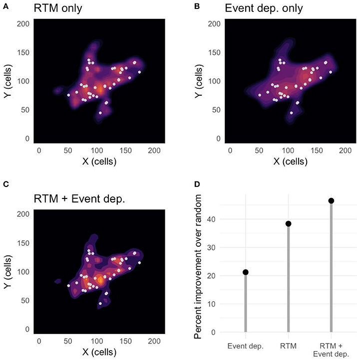
Figure 3. Example of predictions made by (A) the RTM-only model, (B) the event-dependent-only model, and (C) the full (RTM + event dependence) model, against real robbery occurrences (white dots) in Newark, from January 1, 2012 to January 7, 2012. Lighter colors indicate locations in Newark where the models predict a higher likelihood of future robbery occurrences. (D) Shows the improvement that each model provides over a random model without predictive ability, calculated following the procedure described in section Model Performance.

Figure 4 summarizes the results of similar analyzes for predictions over 3, 7, 14, and 28 days for 51 different weeks in 2012 (instead of just the first week of 2012 as in the examples in Figure 3). In each case, the results show that the full model performs significantly better than the random model, the event-dependence-only model and the RTM-only model, in that order (as shown by the non-overlapping notches in the boxplots; Wilcoxon ranked test, all p-values < 0.001).

FIGURE 4

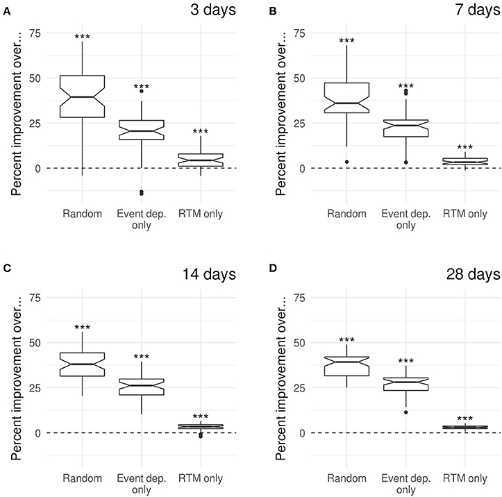
Figure 4. Performance comparison between the full model and the random, event-dependent-only and RTM-only models for predictions at (A) 3 days, (B) 7 days, (C) 14 days, and (D) 28 days. Performance are shown as percent improvement of the full model over each of the other 3 models. Each boxplot corresponds to 51 measurements, each corresponding to the beginning of a different week in 2012. The notches in the boxplots correspond to the 95% confidence interval of the median and them not containing the zero line indicates strong evidence for the median to significantly differ from zero [37]. The symbols above each boxplot correspond to the significance level as calculated using a Wilcoxon ranked test with a null hypothesis of no improvement (ns, non-significant; *p < 0.05; **p < 0.01; ***p < 0.001).

Finally, Figure 5 summarizes a direct comparison between the RTM-only model (the current state of the art in predictive criminology) and the full model that accounts for both event-dependent and environmental influences. For predictions over 1–10 days, for 51 differents weeks in 2012, the full model performs significantly better than the RTM-only model (as shown by the non-overlapping notches in the boxplots; Wilcoxon ranked test, all p-values < 0.001). Note that the variance of the data decreases with the number of days over which the predictions are calculated because of the increasing number of actual robbery occurrences that can be used to compute the average ρ value for each model.

FIGURE 5

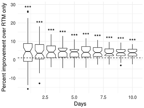
Figure 5. Performance comparison between the full model and the RTM-only model (the current state of the art model in predictive criminology) for predictions at 1–10 days. Performance are shown as percent improvement of the full model over the RTM-only model. Each boxplot corresponds to 51 measurements, each corresponding to the beginning of a different week in 2012. The notches in the boxplots correspond to the 95% confidence interval of the median and them not containing the zero line indicates strong evidence for the median to significantly differ from zero [37]. The symbols above each boxplot correspond to the significance level as calculated using a Wilcoxon ranked test with a null hypothesis of no improvement (ns, non-significant; *p < 0.05; **p < 0.01; ***p < 0.001).

Discussion

We presented in this paper a hybrid approach to model the event-dependent and environmental drivers of criminal behaviors (more specifically robberies) at the scale of a large city (Newark, NJ). This approach combines methods from collective behavior (modeling of dynamic interactions between agents or events) and criminology (risk terrain modeling) to improve forecasting of the emergence and evolution of patterns of criminal activities. The rationale behind this hybrid approach is that RTM—the current state-of-the-art in criminology [4]—does not account for the dependence between successive events, i.e., that the occurrence of a crime at a location increases temporarily the likelihood of future occurrences at or in the neighborhood of that location, independently of other factors such as the environmental makeup. We proposed to complement RTM with a procedure simulating this spatio-temporal event-dependence in order to obtain more accurate forecasting of the changes in the distribution of crime occurrences over time.

The first step of this procedure is to estimate the spatio-temporal dependence between successive events after controlling for environmental influences as estimated using RTM (Figure 1A). Our results (Figure 2) show that, indeed, there is an elevated risk of robbery around previously robbed locations. This increase can be modeled as an inverse function of the distance to the original robbery, and its intensity decreases exponentially with the duration since the original robbery. This is in line with recent studies on hot spots policing that suggest that crime is not randomly distributed and is dependent on events that occurred in close proximity to new ones. For instance, based on a meta-analysis, [25] demonstrated the efficacy of event dependent approaches in increasing the chances that crime can be reduced or prevented in these areas of concentration.

The second step of the procedure uses simulations seeded with historical data to estimate the distribution of future robbery occurrences. In these simulations, the probability of a robbery happening at a location is proportional to the environmental risk at this location (as estimated by risk terrain modeling) modulated by nearby past occurrences (as estimated in the first step of the procedure). In our study, we compare the performance of this hybrid model with the performance of RTM (by setting the event-dependence to zero) and with the performance of an event-dependent only model (by setting the same environmental risk for all cells). This comparison is achieved by measuring the ability of each model to cluster predicted events for a period of time around the location of actual events during that same period of time, relative to a fully randomized model. Our results show that the predictions of the hybrid model are significantly better than the predictions of the other tested models, and that this improvement is maintained over time (at least for predictions up to 4 weeks in the future). The size of the improvement over the RTM-only model may seem limited (4–5% in average) but it is nonetheless significant and can be explained by the quick attenuation of the spatio-temporal influence of past events (see Figure 2) typical of crimes of opportunity such as robberies. Larger effect sizes should be expected for crimes involving stronger interactions between the agents involved. For instance, drug markets and prostitution strolls are more enduring, often locating in the same place over long periods of time, suggesting that social factors work as facilitators in perpetuating these locations as areas of delinquency.

From a criminological perspective, our results suggest that the complexity of crime hotspots in a jurisdiction, which are derived through individual offender activities, do not necessarily require sophisticated individual behavior rules to emerge, persist, or desist. The process can be described probabilistically as a combination of environmental factors and interactions between neighboring successive events. Crimes may not always occur at expected highest-risk places or within existing hotspot areas. But, as time passes, the rational choices and stochasticity of individual offenders' decisions yields a few more crimes at the most “suitable” places. The greater number of crimes at these suitable places induces a greater number (and veracity) of perceptions that these places are “most suitable” to commit crime and reap rewards. Additional crime events stimulate more offenders to choose these places to commit their crimes, and so on Andresen [26].

So, in explaining the clustering of illegally behaving individuals, we view these as a set of dynamic mechanisms whereby hotspots appear at the global level from local interactions among its lower-level components, without being explicitly coded at the individual offender level [14]. In this scenario, positive feedback for a “hotspot cohort” of offenders results from the execution of simple behavioral “rules of thumb” that promote the creation of hotspots. A successful robbery event, for instance, whereby an offender received cash from a victim and was never arrested or punished for it, is a kind of positive feedback which creates the conditions for similar/repeat crimes at the same locale and ultimately clustering at some places, and not others [27]. This is similar to the results of many studies on the aggregation behavior of social animals: they preferentially cluster at favorable locations but, because the individuals are also attracted toward each other, (1) they tend to aggregate at only one or a few among all the favorable locations, and (2) they can sometimes form a stable aggregate at an unfavorable location if a large enough groups has been formed there by chance [16, 18, 28]. In the criminological context, this would explain why not all high-risk locations—as predicted by RTM—become crime hotspots, and why low-risk locations may turn into hotspots in rare cases [11].

By combining environmental and event-dependent influences, our approach suggests a graduated approach to mitigating crime through intervention. At a short timescale, our model predictions can inform practitioners when allocating police resources to places forecasted to be soon in greatest need of mitigation, based on the accumulation of recent crime occurrences. This would (1) help prevent the formation of hotspots by better directing police action and (2) help identify locations to where crime might be displaced after police intervention at an emerging hotspot [29]. On a longer timescale, our ability to identify the environmental drivers of crime may help policy makers better plan the urban and economic development of neighborhoods, either avoiding environmental features that are known to increase risk, or mitigating their effect with those decreasing risk [4, 30].

Conclusion

Malleson et al. [31] argue that modern criminology theory has highlighted the individual-level nature of crime—whereby overall crime rates emerge from individual crimes that are committed by individual people in individual places. However, they say, “traditional modeling methodologies struggle to capture the complex dynamics of the system. The decision whether or not to commit a burglary, for example, is based on a person's unique behavioral circumstances and the immediate surrounding environment.” Malleson et al. [31] add that an effective way to address these problems is through individual-level simulation techniques such as agent-based modeling have begun to spread to the field of criminology. This paper builds on this work and provides new insights into how this approach can advance crime analysis in the future. Indeed, our work:

1. demonstrates that combining event-dependence with environmental predictors enhances our forecasts of future crime over existing methods, even in the case of crime of opportunity—such as robberies—with high attenuation rates;

2. supports the hypothesis that offenders pay attention to the results of previous crime incidences when deciding to commit a crime at a given location;

3. offers a new approach to operationalize and measure risk from exposure (past event) and vulnerability (environment) in assessing their combined spatial influence on crime outcomes and distributions;

Finally, while this approach borrows from the study of collective behaviors in biology, it reciprocates through offering a tested method to forecast behavior accounting for both individual decisions and environmental factors at different spatio-temporal scales. In addition, recent advances in understanding the role individual behavioral modulations and social networks play in shaping the collective behavior of animal groups [32–36] should provide new sources of inspiration for the design of control strategies for place-based policing and community redevelopment efforts.

Author Contributions

SG, LK, and JC: conceived the study; JC: performed the RTM analysis; SG: performed the event-dependence analysis; SG: implemented all the models and performed their analysis and comparison; SG: wrote the manuscript with contributions from LK and JC.

Funding

This work was supported by a grant from the National Institute of Justice (#2016-IJ-CX-K001, Next Generation Risk Terrain Modeling Software: Development and Sustainability). It was also supported by the Initiative for Multidisciplinary Research Teams (IMRT) Award at Rutgers University (Forecasting Crime Emergence and Persistence) and the Rutgers Center on Public Security. The data was obtained as part of a grant from the National Institute of Justice (#2012-IJ-CX-0038, Risk terrain modeling experiment: A multi-jurisdictional place-based test of an environmental risk-based patrol deployment strategy).

Conflict of Interest Statement

The authors declare that the research was conducted in the absence of any commercial or financial relationships that could be construed as a potential conflict of interest.

Supplementary Material

The Supplementary Material for this article can be found online at: https://www.frontiersin.org/articles/10.3389/fams.2018.00013/full#supplementary-material

References

1. Sherman LW, Gartin PR, Buerger ME. Hot spots of predatory crime: routine activities and the criminology of place. Criminology (1989) 27:27–56.

Google Scholar

2. Bowers KJ, Johnson SD. Domestic burglary repeats and space-time clusters: the dimensions of risk. Eur J Criminol. (2005) 2:67–92. doi: 10.1177/1477370805048631

CrossRef Full Text | Google Scholar

3. Brantingham P, Brantingham P. Criminality of place: crime generators and crime attractors. Eur J Crim Policy Res. (1995) 3:5–26. Available online at: https://link.springer.com/article/10.1007%2FBF02242925

Google Scholar

4. Caplan JM, Kennedy LW. Risk Terrain Modeling Manual: Theoretical Framework and Technical Steps of Spatial Risk Assessment for Crime Analysis. Newark, NJ: Rutgers Center on Public Security (2010).

5. Caplan JM, Kennedy LW, Piza EL. Joint utility of event-dependent and environmental crime analysis techniques for violent crime forecasting. Crime Delinquency (2012) 59:243–70. doi: 10.1177/0011128712461901

CrossRef Full Text | Google Scholar

6. Caplan JM, Kennedy LW. Risk Terrain Modeling: Crime Prediction and Risk Reduction. Univ of California Press (2016). Available online at: https://market.android.com/details?id=book-PinlCwAAQBAJ

Google Scholar

7. Kennedy LW, Caplan JM, Piza E. Risk clusters, hotspots, and spatial intelligence: risk terrain modeling as an algorithm for police resource allocation strategies. J Quant Criminol. (2011) 27:339–62. doi: 10.1007/s10940-010-9126-2

CrossRef Full Text | Google Scholar

8. Spelman W. Abandoned buildings: magnets for crime? J. Crim. Justice (1993) 21:481–95. doi: 10.1016/0047-2352(93)90033-J

CrossRef Full Text | Google Scholar

9. Eck JE, Weisburd DL. Crime places in crime theory. In: John E, David E, editors. Crime and Place. Monsey, NY: Criminal Justice Press (1995). p. 1–33.

Google Scholar

10. Johnson SD, Bernasco W, Bowers KJ, Elffers H, Ratcliffe J, Rengert G, et al. Space time patterns of risk: a cross national assessment of residential burglary victimization. J Quant Criminol. (2007) 23:201–219. doi: 10.1007/s10940-007-9025-3

CrossRef Full Text | Google Scholar

11. Kennedy LW, Caplan JM, Piza EL, Buccine-Schraeder, H. Vulnerability and exposure to crime: applying risk terrain modeling to the study of assault in chicago. Appl Spat Anal Policy (2015) 9:529–48. doi: 10.1007/s12061-015-9165-z

CrossRef Full Text | Google Scholar

12. Kennedy LW, Caplan JM. A theory of Risky Places. Newark, NJ: Rutgers Center on Public Security (2012). Available online at: http://www.rutgerscps.org/uploads/2/7/3/7/27370595/risktheorybrief_web.pdf

Google Scholar

13. Camazine S, Deneubourg JL, Franks NR, Sneyd J, Theraulaz G, Bonabeau E. Self-Organization in Biological Systems. Princeton, NJ: Princeton University Press (2001).

Google Scholar

14. Garnier S, Gautrais J, Theraulaz G. The biological principles of swarm intelligence. Swarm Intell. (2007) 1:3–31. doi: 10.1007/s11721-007-0004-y

CrossRef Full Text | Google Scholar

15. Sumpter DJT. The principles of collective animal behaviour. Philos. Trans. R. Soc. Lond. B Biol. Sci. (2006) 361:5–22. doi: 10.1098/rstb.2005.1733

PubMed Abstract | CrossRef Full Text | Google Scholar

16. Deneubourg JL, Lioni A, Detrain C. Dynamics of aggregation and emergence of cooperation. Biol. Bull. (2002) 202:262–7. doi: 10.2307/1543477

PubMed Abstract | CrossRef Full Text | Google Scholar

17. Franks NR, Pratt SC, Mallon EB, Britton NF, Sumpter DJT. Information flow, opinion polling and collective intelligence in house-hunting social insects. Philos. Trans. R. Soc. Lond. B Biol. Sci. (2002) 357:1567–83. doi: 10.1098/rstb.2002.1066

PubMed Abstract | CrossRef Full Text | Google Scholar

18. Jeanson R, Deneubourg JL. Conspecific attraction and shelter selection in gregarious insects. Am. Nat. (2007) 170:47–58. doi: 10.1086/518570

PubMed Abstract | CrossRef Full Text | Google Scholar

19. FBI. Crime in the United States, (2014). U.S. Department of Justice, Federal Bureau of Investigation (2015). Available online at: https://ucr.fbi.gov/crime-in-the-u.s/2014/crime-in-the-u.s.-2014/resource-pages/offense-definitions.pdf

20. Goeman JJ. L1 penalized estimation in the Cox proportional hazards model. Biom. J. (2010) 52:70–84. doi: 10.1002/bimj.20090002

PubMed Abstract | CrossRef Full Text | Google Scholar

21. Stasinopoulos MD, De Bastiani F. Flexible Regression and Smoothing: Using GAMLSS in R. 1st edition. CRC Press/Taylor & Francis Group (2017).

Google Scholar

22. Taylor RB. Social order and disorder of street blocks and neighborhoods: ecology, microecology, and the systemic model of social disorganization. J. Res. Crime Delinq. (1997) 34:113–55.

Google Scholar

23. Taylor RB, Harrell A. Physical Environment and Crime. Washington, DC: US Department of Justice, Office of Justice Programs, National Institute of Justice (1996).

Google Scholar

24. Heffner J. Statistics of the RTMDx utility. Risk Terrain Modeling Diagnostics Utility User Manual (2013), p. 35–39.

25. Braga AA, Papachristos AV, Hureau DM. The effects of hot spots policing on crime: an updated systematic review and meta-analysis. Justice Q. (2014) 31: 633–63. doi: 10.1080/07418825.2012.673632

CrossRef Full Text | Google Scholar

26. Andresen M. A. Environmental Criminology: Evolution, Theory, and Practice. Taylor & Francis (2014). Available online at: https://books.google.com/books?id=8bgTAwAAQBAJ

Google Scholar

27. Bernasco W, Block R. Robberies in Chicago: a block-level analysis of the influence of crime generators, crime attractors, and offender anchor points. J Res Crime Delinq. (2011) 48:33–57. doi: 10.1177/0022427810384135

CrossRef Full Text | Google Scholar

28. Canonge S, Sempo G, Jeanson R, Detrain C, Deneubourg JL. Self-amplification as a source of interindividual variability: shelter selection in cockroaches. J. Insect Physiol. (2009) 55:976–82. doi: 10.1016/j.jinsphys.2009.06.011

PubMed Abstract | CrossRef Full Text | Google Scholar

29. Piza EL, Kennedy LW, Caplan JM. Facilitators and impediments to designing, implementing, and evaluating risk-based policing strategies using risk terrain modeling: insights from a multi-city evaluation in the United States. Eur J Crim Policy Res. (2018) 1–25. doi: 10.1007/s10610-017-9367-9

CrossRef Full Text | Google Scholar

30. Kennedy LW, Caplan JM, Piza EL. A Multi-Jurisdictional Test of Risk Terrain Modeling and Place-Based Evaluation of Environmental Risk-Based Patrol Deployment Strategies (2015). Available online at: http://www.rutgerscps.org/uploads/2/7/3/7/27370595/nij6city_results_inbrief_final.pdf

31. Malleson N, Heppenstall A, See L, Evans A. Using an agent-based crime simulation to predict the effects of urban regeneration on individual household burglary risk. Environ. Plann. B Plann. Design (2013) 40:405–26. doi: 10.1068/b38057

CrossRef Full Text | Google Scholar

32. Becker J, Brackbill D, Centola D. Network dynamics of social influence in the wisdom of crowds. Proc Natl Acad Sci U.S.A. (2017) 114:E5070–E5076. doi: 10.1073/pnas.1615978114

PubMed Abstract | CrossRef Full Text | Google Scholar

33. Bode NWF, Wood AJ, Franks DW. The impact of social networks on animal collective motion. Anim. Behav. (2011) 82:9–38. doi: 10.1016/j.anbehav.2011.04.011

CrossRef Full Text | Google Scholar

34. Michelena P, Jeanson R, Deneubourg JL, Sibbald AM. Personality and collective decision-making in foraging herbivores. Proc R Soc B Biol Sci. (2010) 277:1093–1099. doi: 10.1098/rspb.2009.1926

PubMed Abstract | CrossRef Full Text | Google Scholar

35. Pruitt JN, Keiser CN. The personality types of key catalytic individuals shape colonies' collective behaviour and success. Anim. Behav. (2014) 93:87–95. doi: 10.1016/j.anbehav.2014.04.017

CrossRef Full Text | Google Scholar

36. von Rueden C, Gavrilets S, Glowacki L. Solving the puzzle of collective action through inter-individual differences. Philos. Trans. R. Soc. Lond. B Biol. Sci. (2015) 370:20150002. doi: 10.1098/rstb.2015.0002

PubMed Abstract | CrossRef Full Text | Google Scholar

37. Chambers JM, Cleveland WS, Kleiner B, Tukey PA. Comparing Data Distributions. New York, NY: Chapman & Hall (1983).

Google Scholar