 Chen-Yun Lin
 Arin Minasian2
- 1Department of Mathematics, Duke University, Durham, NC, United States
- 2Department of Electrical Engineering, University of Toronto, Toronto, ON, Canada
- 3Department of Mathematics, University of Toronto, Toronto, ON, Canada
- 4Department of Statistical Science, Duke University, Durham, NC, United States
- 5Mathematics Division, National Center for Theoretical Sciences, Taipei, Taiwan
In this paper, we propose a novel principal bundle model and apply it to the image denoising problem. This model is based on the fact that the patch manifold admits canonical groups actions such as rotation. We introduce an image denoising algorithm, called the diffusive vector non-local Euclidean median (dvNLEM), by combining the traditional nonlocal Euclidean median (NLEM), the rotational structure in the patch space, and the diffusion distance. A theoretical analysis of dvNLEM, as well as the traditional nonlocal Euclidean median (NLEM), is provided to explain why these algorithms work. In particular, we show how accurate we could obtain the true neighbors associated with the rotationally invariant distance (RID) and Euclidean distance in the patch space when noise exists, and how we could apply the diffusion geometry to stabilize the selected metric. The dvNLEM is applied to an image database of 1,361 images and a comparison with the NLEM is provided. Different image quality assessments based on the error-sensitivity or the human visual system are applied to evaluate the performance.
1. Introduction
A widely accepted approach to model the low dimension structure is by considering the manifold; that is, we assume that the collected dataset, while might be of high dimension, is located on a low dimensional manifold [1–3]. Under this assumption, several algorithms were proposed toward this goal, like isomap [1], locally linear embedding [4], eigenmaps (EM) [2], diffusion maps [3], Hessian LLE [5], vector diffusion maps [6, 7], non-linear independent component analysis or empirical intrinsic geometry [8, 9], alternating diffusion [10, 11], horizontal diffusion maps [12] etc.
One example of such model is the patch manifolds. It is well-known that the non-local mean (NLM) [13] algorithm leads to a better edge preservation [14], and this improvement is directly related to the diffusion process on the nonlinear geometric structure [15]. One can further consider the rotational structure of patch spaces to denoise images [16–21]. Two patches are viewed the same or called rotationally invariant, if they are the same up to rotation. While the patch space model and diffusion-based algorithms have been successfully applied to different fields, such as the inpainting problem [22–25] and the medical imaging problem [19, 26, 27], however, to the best of our knowledge, a companion theoretical study is lacking. It is not clear how we could correctly find the neighbors when noise exists, and why the patch size should be neither too big nor too small and thus why patch space approaches are better than pixel-based ones.
In this paper, we focus on the idea of manifold learning via the principal bundle approach and its associated theoretical analysis. We model the patch space by a principal bundle so that rotationally invariant patches are modeled by fibers diffeomorphic to SO(2). We further show that with high probability, which depends on the patch size and the noise level, one could accurately determine the neighborhood from the noisy patches (Theorem 3.2 and Remark 3.3). We apply it to the image denoising problem and propose an image denoising algorithm, dvNLEM. Although the results indicate that a suitable chosen patch size enhance the neighbor search accuracy, the error is inevitable. We then further stabilize the above theoretical results by applying the diffusion distance (DD), which has been theoretically proved to be robust to noise [28]. Based on the theoretical understanding, we consider the diffusive vector nonlocal Euclidean median (dvNLEM) algorithm that combines the rotational alignment, the DD, and the median. In the dvNLEM, we consider the RID where the RID of two rotationally invariant patches is 0. To reduce the noise influence, the RID is further stabilized by the DD. With the DD, we determine the neighboring patches, and evaluate the median value of the central pixels of all neighboring patches. To overcome this computational intensity, we use scale-invariant feature transform (SIFT) features as a relaxation step to estimate the neighbors.
2. Mathematical Model
For the i-th pixel on a given grayscale image I ∈ ℝN × N and an odd integer q, we associate it with a patch Pi of size q × q centerd at the i-th pixel. If the i-th pixel is close to the boundary of I, we pad the image by 0 and generate the corresponding patch. Denote the set of all patches as To express the notation in a compact format, we stack the columns of the matrix I into a vector I∨ ∈ ℝN2, where the ((ℓ−1)N+1)-th to the (ℓN)-th entries in I∨ is the ℓ-th column of I, where ℓ = 1, …, N. We represent the image I and patches Pi in the matrix form and the column form interchangeably.
For a clean image I(c), we represent its noisy image as
the i-th clean patch as and its associated noisy patch as
where ξi is additive Gaussian white noise with mean 0 and standard deviation 1.
Definition 2.1. The rotationally invariant distance (RID) between two patches, Pi and Pj is defined as
where || · || denotes the ℓ2 norm and O.Pj means rotating the patch P by O.
By identifying patches up to rotation, we make the following assumption. First, recall the definition of a fiber bundle with group structure G [29].
Definition 2.2 (Fiber bundle with group structure G). Let F and M be manifolds. A fiber bundle E with fiber F over M consists of a topological space E together with a map π : E : → M satisfying the local triviality condition. Let G be a Lie group, for example the rotation group SO(2). Let the map.: G × F → F be a smooth left action of F. That is, the map (the action of G).: (x, g) ↦ g.x from G × F to F satisfies
where e is the neutral element of G and
This group G is often called the gauge group or the transition group. If the fiber is equal to the structure group, then (π, E, M, G) is called a principal G bundle. See Definition 5.7 in Gallier [30]. This definition is equivalent to the definition of principal bundle requiring G as a right action on E. See, Propositions 5.5 and 5.6 in Gallier [30]. Suppose P : ℝ2 → ℝ represents a patch. For O ∈ SO(2) and s ∈ ℝ2 expressed by a column vector, we define the action on P as
This is a left group action since for any O1, O2 ∈ SO(2),
Since each fiber, including a patch and its rotated patches, can be identified as S1, and SO(2) is diffeomorphic to S1, the patch space could be viewed as a principal SO(2) bundle.
Assumption 2.3 (SO(2)-principal bundle). The patch space is a finite subset of the fiber bundle E with π : E → M and a left SO(2) group action so that the quotient space is a finite subset of the corresponding base manifold.
Note that the SO(2) action preserves the fiber that is diffeomorphic to SO(2). In Supplementary Material, we further discuss how patch spaces naturally carry principal bundle structures.
3. Theoretical Analysis
The theoretical findings below show that with high probability, the clean patch neighbors could be “accurately” evaluated from the noisy patch neighbors with respect to RID. Lemma 3.1 gives that the square distance between non-overlapping patches is distributed according to a non central chi-squared distribution. We approximate the square distance between overlapping patches by a chi-squared distribution. Theorem 3.2 gives the large deviation bound for the RID, which allows us to take the RID into account to denoise the image. If we omit the rotation action, then we obtain the large deviation bound for the Euclidean distance (Corollary 3.4), which explains why the traditional NLM/NLEM algorithms work.
We introduce the following sets associated with and , and O ∈ SO(2):
whose cardinality is the size of the overlapping pixels;
which is associated with the “swapped” pixel indices after rotation; and
which is associated with the overlapped pixels with “identical indices” after rotation and depends on O. By definition, KI(O) ⊆ KS(O) ⊆ KO(O). Note that KI(O) has only at most one element. For the NLEM, KI(O) and KS(O) are both empty.
Lemma 3.1. For any two patches and and a fixed O, denote and .
1. If and are disjoint, then is a noncentral χ2 random variable with q2 degrees of freedom and non-centrality parameter .
2. If and overlap, then
Moreover, X can be approximated by , where
Since , is a biased estimator of . When two patches overlap, depending on the clean patches' structure, the RID estimator from the noisy patches might be biased toward overlapped patches. Thus, if the overlapping patches are included in the denoising process, the search of the nearest neighboring patches might be biased to the “local patches” that have overlaps.
Theorem 3.2. Suppose and are disjoint patches and σq < ϵ. If , then
which decreases as q decreases. If , then
which decreases as q increases.
Remark 3.3. For overlapping patches, can be approximated by where c and f are given by (13). By direct computation, one can see c decreases and the degree of freedom f increases as q increases. This suggests similar conclusion as in Theorem 3.2 due to the behaviour of chi-squared distributions. That is, if , the tail-area probability decreases as q increases; if , then decreases as q increases.
The above observations suggest that we need to choose a suitable patch size q to rule out unwanted patches and keep desired patches. In practice, we found that an odd value q between 7 and 15 leads to a good performance, but the optimal q depends on the image. If O is the identity, the same argument explains why the ℓ2 distance between two clean patches could be well approximated by noisy patches.
Corollary 3.4. Suppose and are disjoint patches and σq < ϵ. If , then
which decreases as q decreases. If , then
which decreases as q increases.
The quantity σ2q2 could be understood as the “total energy” of the added noise, and the condition σ2q2 < ϵ2 means that the RID estimated from two noisy patches is controlled by the square root of the energy of the noise. With this energy viewpoint, we could apply the technique developed in El Karoui and Wu [28]. However, we carried out the proof in the above way to emphasize the main purpose of the RID, and to find the true neighbors and the dependence on the patch size.
Before closing this section, we mention that even if by choosing suitable patch size we could more accurately find the neighbors, the error is inevitable. Thus, to further find correct neighbourhoods, we need more tools to stabilize the found neighbors. In this work, we apply the diffusion geometry framework to stabilize the RID for the image denoising purpose, which is detailed in the next section.
4. Diffusive Vector Non-local Euclidean Median Algorithm
Take a clean grayscale image denoted as I(c) ∈ ℝN × N normalized to be of mean 0 and standard deviation 1. Take the associated noisy image I(n), the noisy patches with σ > 0. The goal of the denoising problem is finding an algorithm that will recover I(c) from I(n) as accurately as possible. Based on the theoretical analysis shown in section 3, we now discuss the dvNLEM algorithm.
4.1. dvNLEM Algorithm
Theorem 3.2 essentially says that even when noise exists, we could still find the true neighbors with the RID with high probability; in other words, it is possible to find wrong neighbors. Based on the principal bundle model, we apply the diffusion map and the DD to “filter out” wrong neighbors and improve the overall accuracy. The idea is to combine the fiber bundle structure underlying the patch space with the diffusion map (DM). With the RID, define the affinity matrix W ∈ ℝN2 × N2 by
where i, j = 1, …, N2 and ϵ > 0 is the pre-determined bandwidth. With the affinity matrix W, the graph Laplacian and the associated transition matrix. A = D−1W where D is the degree matrix which is diagonal and defined as By taking the top m eigenvalues and eigenvectors of the transition matrix, we then embed each patch into a low-dimensional space via the DM (24) and calculate the DD to evaluate the true neighbors of each patch. For each patch , we identify its N1 ∈ ℕ nearest neighbors in the sense of DD and denote this set as NDD(i). Based on the robustness property of the DM [28, 31], this step acts as an additional filtering procedure to dismiss the patches in the initial nearest neighbors set determined by the RID. The denoised image, denoted as Ĩ(dvNLEM) ∈ ℝN×N.
If we identify a patch its N1 ∈ ℕ nearest neighbors associated with the RID instead of DD, denoted as NRID(i), and denoise the noisy image by the Euclidean median, we obtain an intermittent denoising algorithm, which we call the vector nonlocal Euclidean median (vNLEM) and denote the denoised image as Ĩ(vNLEM).
4.1.1. Numerical Techniques to Speed Up the Computation–Search Window
While the proposed algorithm seems a straightforward generalization of the NLM/NLEM/NLPR, there are numerical issues we have to handle.
Obtaining the pairwise distances between all pairs of patches is computationally intense and time-consuming. One practical solution is to only consider a pre-assigned number of nearest neighbors. By doing so, we simultaneously reduce the computational time and the memory required to save W.
We further limit our algorithm to consider only patches within a given search window centered at the reference patch. For a patch , we consider the search window of size (2N2 + 1) × (2N2 + 1) centered at the patch
where N2 ∈ ℕ so that (2N2 + 1) × (2N2 + 1) > N1. With this search window, we form the affinity matrix by the following:
4.1.2. Numerical Techniques to Improve the RID Evaluation–SIFT
Finding the RID between two given patches incurs huge computational costs. Also, performing a direct numerical rotation might lead to a non-negligible error and deviate the estimated RID. To alleviate these two troubles and facilitate the derivation of the affinity matrix, we use the scale invariant feature transform (SIFT) [32] to approximate the RID. We could consider the central moments [16, 17, 19], the curvelet transform [21], or the Fast Affine Template Match [33] algorithm, to capture the rotational feature. To simplify the discussion, we focus on the SIFT algorithm.
The particular feature we extract by SIFT is the orientation feature. For each pixel, based on the local image gradient direction, an orientation angle is calculated and assigned. We use this orientation to approximate the RID distances between the patches. Denote the orientation for the center of as . The relative angle between and achieving the RID is approximated by . We then rotate by , where Rθ ∈ SO(2) means the rotation by θ degrees. Next, we perform the exhaustive search over a small range centered around the estimated angular relationship :
where is the chosen upsampling operator that increases the sampling rate of the patch by k ∈ ℕ times and θl > 0 is the parameter chosen by the user. The use of Uk is to improve the accuracy of numerical rotation. Hence the estimated RID is
We use the following affinity weights in (25):
4.1.3. The Proposed dvNLEM Algorithm
The proposed algorithms after the above modifications are summarized in Algorithm 1. We slightly abuse the terminology and also call the modified denoising scheme in (25) based on the estimated DD the dvNLEM and denote Ĩ(dvNLEM) as the denoised image by dvNLEM. Similarly, we call the modified denoising scheme in (23) based on the approximated RID (22) the vNLEM algorithm and denote Ĩ(vNLEM) as the denoised image by vNLEM.
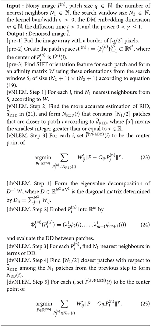
Algorithm 1. Diffusive vector non-local Euclidean median algorithm
5. Image Quality Assessment
In the literature, the denoising performance is commonly evaluated by the “error-based” measurements, such as the signal-to-noise ratio (SNR) or the peak SNR. However, it is well known that those error-based quantities might capture only partial information of the image quality. In this study, we consider different image quality assessment (IQA) methods that additionally take different aspects of the image into account, like the human visual system, to evaluate the performance of different denoising algorithms. IQA is an important subfield in image processing. The goal is to find an index quantifying “how good” an image is that is suitable for different scenarios. We consider measures of two major. The first category consists of objective measures based on a chosen theoretical model without taking the human visual system (HVS) into account. The second category consists of objective measures based on models taking the HVS into account. Below we summarize these measures. Denote the clean image as I ∈ ℝN × N. We are concerned with how close the noisy observation I + σ ξ is to I, or the denoised image Ĩ is to I.
The SNR and peak-signal-to-noise ratio (PSNR) belong to the first category.
While SNR and PSNR are widely applied IQA's in the field, they do not necessarily tell us all aspects of how well the denoising methods performed. For example, they do not readily capture the edge preserving capability of an algorithm.
To capture the edge preservation performance, we consider the third measurement, the Sobolev index [34], which also belongs to the first category. Let Î and denote the discrete Fourier transforms of I and Ĩ, respectively. The Sobolev index of order κ is then defined by the Sobolev norm, and is given by
where Ω is the lattice of the frequency domain and ηω is the two-dimensional frequency vector associated with ω ∈ Ω.
We further consider the earth mover's distance (EMD) [35]. The EMD between two probability distributions μ and ν on ℝ is defined as
where is the cumulative distribution function of μ and similarly for fν. We will evaluate the EMD to compare how close the distribution of the estimated noise is to the added noise.
While the above measurements have been widely applied in different problems and provide useful information, it has been well-accepted that they do not capture all aspects from the perspective of image quality. In generally, it is not statistically consistent with human observers [36].
Several metrics have been designed in the past decades to faithfully take the HVS into account. These metrics emphasize the importance of luminance, the contrast, and the frequency/phase content. We consider the state-of-art measurement the Feature SIMilarity (FSIM) index [36] in this category. The FSIM is based on the model that the HVS perceives an image mainly based on its low-level features, such as edges and zero crossings, and it separates the similarity measurement task into phase congruency and gradient magnitude. Here we summarize the FSIM index. Suppose the dynamical range of the image is . The definition of FSIM depends on the definition of the phase congruency and gradient magnitude. The phase congruent of I at i, denoted as PI(i), and the gradient magnitude of I at i, denoted as GI(i), are defined in Zhang et al. [36]. Similarly, we can define PĨ(i) and GĨ(i). The FSIM between I and Ĩ is defined as
where
and
Here, we follow [36] and choose T1 = 0.85 and T2 = 160. There are several other measures of this kind in the field, and we refer interested readers to Zhang et al. [36] and Wang et al. [37] for a review of these indices.
6. Numerical Result
We fix the following parameters for NLEM, vNLEM, and dvNLEM for a fair comparison. Fix q = 13. We build 13 × 13 patches around each pixel of the noisy image. We chose ϵ = (16.5)2, the number of nearest neighbors as N1 = 100, the size of the search window for creating the initial affinity matrix is determined by N2 = 10; that is, 21 × 21 neighbours in each the search window. The θl in (20) is set to 30 degrees, the upsampling operator Uk is implemented by the bicubic interpolation, and k is set to 2. After building the transition matrix, we choose m = 30 to evaluate the DM and DD. We select γ = 0.1 for the final denoising step. The Matlab code is available via request.
To compare our results with those of the NLEM algorithm, we also preformed the NLEM denoising with ϵ = (6.5)21 with the same patch size q = 13 and search window 21 × 21. The kernel bandwidth is chosen to give the best performance for the NLEM algorithm in terms of SNR and PSNR.
In Table 1 we report the different IQA metrics, including SNR, PSNR, RMS, SOB, OT, and FSIM discussed previously as well as the computational time, by running the three denoising algorithms on 1,361 sample images of size 512 × 5122. There are 98 images for animals, 143 images for flowers, 52 images for fruits, 115 images for landscapes, 450 images for faces, 419 images for manmade structures, and 44 miscellaneous images. The SOB metric is applied to the image recovery error. This measure particularly reflects the amount of edge information wiped out due to the denoising process. Therefore, the scheme with a lower SOB index performs the better. For the other indices, the higher the index is, the better the performance is. Under the null hypothesis that the performance of two algorithms is the same, we reject the hypothesis by the Mann–Whitney U-test with the p value less than 10−4. Note that based on the overall statistics, VNELM and dvNLEM outperform NLEM statistically significantly on all IQA metrics. On the other hand, we cannot distinguish the performance of vNLEM and dvNLEM statistically, except on the FSIM index. This result suggests that dvNLEM could better recover features sensitive to HVS.
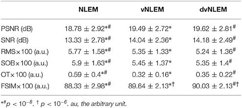
Table 1. Summary statistics over 1,361 images of different denoising algorithms evaluated by different image quality assessment metrics.
The execution times based on 17 images are 501.8 ± 203.3, 1489.8 ± 26.1, and 1619 ± 34.8 s for NLEM, vNLEM, and dvNLEM, respectively. This execution time is obtained on a PC with 8 Gb of RAM using a single core from Intel Corei7 CPU with a clock speed of 3.7 GHz running on Microsoft Windows 7.
6.1. Application to the Cytometry Problem
In this last example, we apply the vNLEM and dvNLEM to the third-harmonic-generation (THG) microscopy image. The goal of the THG microscopy-based imaging cytometry is to automatically differentiate and count different types of blood cells with less blood ex vivo, or even in vivo [38]. One of the many strengths of THG is reflecting the granularity of leukocytes, which allows us to apply image processing techniques for the automatic classification. However, the raw data is noisy most of time, and a denoising technique is needed. We now apply the NLEM, vNLEM, and dvNLEM to the THG sectioning image of the whole blood smear at 1 hour post blood sampling. The data is provided by Professor Tzu-Ming Liu, Faculty of Health Sciences, University of Macau. The result is shown in Figure 1. Note that since we do not have the “ground truth” for a comparison, we only show the FSM for the quality evaluation purpose. While the result is encouraging, a systematical study of the problem, and a systematic comparison of the proposed algorithm with existing algorithms is needed. The result will be reported in a future work.
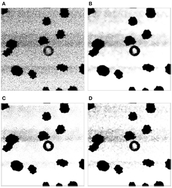
Figure 1. The cytometry image. Since the “ground truth” is not available for a comparison, we only show the FSIM for the quality evaluation purpose. (A) Original image. (B) NLEM, FSIM = 0.947. (C) vNLEM, FSIM = 0.967. (D) dvNLEM, FSIM = 0.97.
7. Conclusion and Discussion
In this paper, a principal bundle structure is applied to model the patch space and describe the rotational structure, based on which a theoretical analysis of the RID is provided to explain how accurate we could obtain the true neighbors when noise exists. Based on the well studied DD, the RID could be further stabilized when noise exists; that is, we nonlinearly filter out the wrongly found nearest neighbors. The theoretical result also serves as an explanation of why NLM and NLEM work well. The theoretical results lead to an image denoising algorithm, vNLEM and dvNLEM, by combining the traditional NLEM, the rotational structure in the patch space, and the DD. Numerically, we apply the commonly applied SIFT as a relaxation step to estimate the rotational alignment. The numerical simulation provides positive evidence of the potential of the proposed algorithm. The potential of the proposed model, algorithms, and the associated theory are statistically supported by a large image database composed of 1,361 images. Below, we discuss the limitations of the current work and several future works.
First, the computational complexity needs to be further improved. Note that the main difference between the vNLEM/dvNLEM and the NLEM algorithms is the chosen metric. In the vNLEM, there is no fast algorithm yet to determine the nearest neighbors with respect to the RID, to the best of our knowledge. Although we have delegated the problem of evaluating the RID distance to that of evaluating the SIFT distance, the numerical performance still has a significant room for improvement.
Second, although the manifold model has been widely accepted in the field, and the DD applied in dvNLEM is based on the manifold structure, it is certainly arguable if in general a patch space could be well approximated by a manifold. On one hand, we might need different models, and hence different metrics, for different kinds of images. For example, while the RID helps reduce the dimension of the patch space of a “structured” image, its deterministic nature might render it unsuitable for analyzing a “texture” image, since the texture features are stochastic in nature. In short, it might be beneficial to take the metrics designed for the texture analysis into account. On the other hand, we could consider to segment the given noisy image into different categories, and run the vNLEM on each category. This segmentation step is related to the “multi-manifold model” considered in the literature [39, 40], and could be understood as a generalization of the search window method used in this paper.
Third, we should consider different structures in the denoising procedure. In addition to taking the rotation group to fibrate the patch space, it is an intuitive generalization to further consider other groups, like the dilation group or even the general linear group. Also, while the current work focuses on grayscale images, the proposed algorithm has the potential to be generalized to colored images. In colored images, more structures, like the color space, will be taken into account. Furthermore, in practice we would expect to have more than one image from the practical problem. Under the assumption that the noise behavior is similar, it is of great interest to see if we could further improve the denoise performance by denoising multiple available images simultaneously.
Fourth, note that the proposed algorithm could be understood as aiming to reduce the error introduced to the clean image. However, it has been widely argued in the IQA society that simply reducing the error might not lead to the optimal result in all scenarios. It might be more important to take the human perception into account, if the images are meant to be watched by a human being. While the proposed vNLEM provides a satisfactory result by the FSIM evaluation, note that the “features” considered in the FSIM are not used in the algorithm. It is reasonable to expect that by taking these features into account, we could further improve the result.
Fifth, in this paper we focus only on comparing our algorithm with the NLEM and study the corresponding theoretical properties and the geometric structure of the underlying patch space model. For the image denoising purpose, there are several other image denoising algorithms available in the field, and we will do a systematic comparison in a upcoming report. For example, while not specifically indicated, the widely used algorithm BM3D [41] and its generalizations, for example [42], and BPFA are also based on the patch space model. We could view the sparsity structure used in BM3D and the Bayesian approach in BPFA as a different way to design a “metric” to compare different patches.
Last but not least, although we compared the algorithm on a big image database and reported the statistical significance, note that statistical significance does not imply practical significance. Particularly, the included images are not exhaustive. A more systematic comparison is thus needed. Furthermore, we do not claim that the proposed denoise algorithm is better than any of the state-of-the-art image denoising algorithm, like the BM3D. In practice, the overall performance depends on the problems encountered, and the specific applications, like the cytometry problem, and a systematic comparison with other algorithms will be discussed in a upcoming research report.
Author Contributions
AM and XQ contribute to the code implementation. C-YL and H-TW contribute to the theoretical development and manuscript preparation.
Funding
H-TW's research is partially supported by Sloan Research Fellow FR-2015-65363 and partially by Connaught New Researcher grant 498992.
Conflict of Interest Statement
The authors declare that the research was conducted in the absence of any commercial or financial relationships that could be construed as a potential conflict of interest.
Acknowledgments
H-TW would like to thank the valuable discussions with Professor Ingrid Daubechies and Professor Amit Singer. C-YL would like to thank Professor Chiahui Huang for her helpful discussions. The authors would like to thank Professor Tzu-Ming Liu for sharing the cytometry image. H-TW's research is partially supported by Ministry of Science and Technology 107-2119-M-002-016-, NCTS Taiwan.
Supplementary Material
The Supplementary Material for this article can be found online at: https://www.frontiersin.org/articles/10.3389/fams.2018.00021/full#supplementary-material
Footnotes
1. ^The code is available in https://www.mathworks.com/matlabcentral/fileexchange/40624-non-local-patch-regression
2. ^The images are collected from :
• Caltech-UCSD Birds-200-2011 collection at : http://www.vision.caltech.edu/visipedia/CUB-200-2011.html
• Digital Image Processing, 3rd ed, by Gonzalez and Woods at : http://www.imageprocessingplace.com/DIP-3E/dip3e_book_images_downloads.htm
• USC-SIPI image database at: http://sipi.usc.edu/database/
References
1. Tenenbaum JB, de Silva V, Langford JC. A global geometric framework for nonlinear dimensionality reduction. Science (2000) 290:2319–23. doi: 10.1126/science.290.5500.2319
2. Belkin M, Niyogi P. Laplacian eigenmaps for dimensionality reduction and data representation. Neural Comput. (2003) 15:1373–96. doi: 10.1162/089976603321780317
3. Coifman RR, Lafon S. Diffusion maps. Appl Comput Harmon Anal. (2006) 21:5–30. doi: 10.1016/j.acha.2006.04.006
4. Roweis ST, Saul LK. Nonlinear dimensionality reduction by locally linear embedding. Science (2000) 290:2323–6. doi: 10.1126/science.290.5500.2323
5. Donoho DL, Grimes C. Hessian eigenmaps: locally linear embedding techniques for high-dimensional data. Proc Natl Acad Sci USA. (2003) 100:5591–6. doi: 10.1073/pnas.1031596100
6. Singer A, Wu HT. Vector diffusion maps and the connection laplacian. Commun Pure Appl Math. (2012) 65:1067–144. doi: 10.1002/cpa.21395
7. Singer A, Wu HT. Spectral convergence of the connection Laplacian from random samples. Inf Infer. (2017) 6:58–123. doi: 10.1093/imaiai/iaw016
8. Singer A, Coifman RR. Non-linear independent component analysis with diffusion maps. Appl Comput Harmon Anal. (2008) 25:226–39. doi: 10.1016/j.acha.2007.11.001
9. Talmon R, Coifman RR. Empirical intrinsic geometry for intrinsic modeling and nonlinear filtering. Proc Nat Acad Sci USA. (2013) 110:12535–40. doi: 10.1073/pnas.1307298110
10. Lederman RR, Talmon R. Learning the geometry of common latent variables using alternating-diffusion. Appl Comput Harmon Anal. (2015) 44:509–36. doi: 10.1016/j.acha.2015.09.002
11. Talmon R Wu HT. Discovering a latent common manifold with alternating diffusion for multimodal sensor data analysis. Appl Comput Harmon Anal 2018.
12. Gao T. The Patch Manifolds of Many Natural Images Have Low Dimensional Structure. Available online at: https://arxiv.org/pdf/1602.02330.pdf (2016).
13. Buades A, Coll B. A non-local algorithm for image denoising. In: IEEE Computer Society Conference on Computer Vision and Pattern Recognition. San Diego, CA (2005) p. 60–5.
14. Jain P, Taygi V. A survey of edge-preserving image denoising methods. Inf Syst Front. (2016) 18:159–70. doi: 10.1007/s10796-014-9527-0
15. Singer A, Shkolnisky Y, Nadler B. Diffusion interpretation of nonlocal neighborhood filters for signal denoising. SIAM J Imaging Sci. (2009) 2:118–39. doi: 10.1137/070712146
16. Zimmer S, Didas S, Weickert J. A rotationally invariant block matching strategy improving image denoising with non-local means. In: Proc 2008 Int Workshop on Local and Non-local Approximation in Image Processing, LNLA 2008 Lausanne (2008).
17. Grewenig S, Zimmer S, Weickert J. Rotationally invariant similarity measures for nonlocal image denoising. J Vis Commun Image Represent. (2011) 22:117–30. doi: 10.1016/j.jvcir.2010.11.001
18. Qi X. Vector Nonlocal Mean Filter. Toronto, ON: University of Toronto (2015). Available online at: Http://hdl.handle.net/1807/70528
19. Guizard N, Coupe P, Fonov VS, Manjon JV, Arnold DL, Collins DL. Rotation-invariant multi-contrast non-local means for MS lesion segmentation. Neuroimage (2015) 8:376–89. doi: 10.1016/j.nicl.2015.05.001
20. Sreehari S, Venkatakrishnan SV, Drummy LF, Simmons JP, Bouman CA. Rotationally-invariant non-local means for image denoising and tomography. In: International Conference on Image Processing (ICIP) Quebec City, QC (2015).
21. Zhang D, He J, Du M. Image restoration via patch orientation-based low-rank matrix approximation and nonlocal means. J Electron Imaging (2016) 25:023021. doi: 10.1117/1.JEI.25.2.023021
22. Gepshtein S, Keller Y. Image completion by diffusion maps and spectral relaxation. In: IEEE Transactions on Image Processing : A Publication of the IEEE Signal Processing Society (2013) p. 2983–94. doi: 10.1109/TIP.2013.2237916
23. Osher S, Shi Z, Zhu W. Low Dimensional Manifold Model for Image Processing. Tech report, UCLA, Tech Rep CAM report 1604. (2016).
24. Yin R, Gao T, Lu Y, Daubechies I. A tale of two bases: local-nonlocal regularization on image patches with convolution framelets. SIAM J Imaging Sci. (2017) 10:711–50. doi: 10.1137/16M1091447
25. Zhou M, Chen H, Paisley J, Ren L, Li L, Xing Z, et al. Nonparametric bayesian dictionary learning for analysis of noisy and incomplete images. IEEE Trans Image Process. (2012) 21:130–44. doi: 10.1109/TIP.2011.2160072
26. Chan C, Fulton R, Feng DD, Meikle S. Median non-local means filtering for low SNR image denoising: application to PET with anatomical knowledge. In: IEEE Nuclear Science Symposium Conference Record. (2010) p. 3613–8. doi: 10.1109/NSSMIC.2010.5874485
27. Manjón JV, Coupé P, Buades A, Louis Collins D, Robles M. New methods for MRI denoising based on sparseness and self-similarity. Med Image Anal. (2012) 16:18–27. doi: 10.1016/j.media.2011.04.003
28. El Karoui N, Wu HT. Connection graph Laplacian methods can be made robust to noise. Ann Stat. (2016) 44:346–72. doi: 10.1214/14-AOS1275
29. Eguchi T, Gilkey PB, Hanson AJ. Gravitation, gauge theories and differential geometry. Phys Rep. (1980) 66:213–393.
30. Gallier J. Notes On Group Actions Manifolds, Lie Groups and Lie Algebras (2005). Available online at: http://www.cis.upenn.edu/~cis610/lie1.pdf (Accessed November 21 2016).
31. El Karoui N. On information plus noise kernel random matrices. Ann Stat. (2010) 38:3191–216. doi: 10.1214/10-AOS801
32. Lowe DG. Distinctive image features from scale-invariant keypoints. Int J Comput Vis. (2004) 60:91–110. doi: 10.1023/B:VISI.0000029664.99615.94
33. Korman S, Reichman D, Tsur G, Avidan S. Fast-match: fast affine template matching. Int J Comput Vis. (2017) 121:111–25. doi: 10.1007/s11263-016-0926-1
34. Wilson DL, Baddeley AJ, Owens RA. A new metric for grey-scale image comparison. Int J Comput Vis. (1997) 24:5–17.
35. Villanic C. Topics in Optimal Transportation. Graduate Studies in Mathematics; American Mathematical Society (2003).
36. Zhang L, Zhang L, Mou X, Zhang D. FSIM: a feature similarity index for image quality assessment. IEEE Trans Image Process. (2011) 20:2378–86. doi: 10.1109/TIP.2011.2109730
37. Wang Z, Bovik AC, Sheikh HR, Simoncelli EP. Image quality assessment: from error visibility to structural similarity. IEEE Trans Image Process. (2004) 13:600–12. doi: 10.1109/TIP.2003.819861
38. Wu CH, Wang TD, Hsieh CH, Huang SH, Lin JW, Hsu SC, et al. Imaging cytometry of human leukocytes with third harmonic generation microscopy. Sci Rep. (2016) 6:37210. doi: 10.1038/srep37210
39. Yang W, Sun C, Zhang L. A multi-manifold discriminant analysis method for image feature extraction. Pattern Recogn. (2011) 44:1649–57. doi: 10.1016/j.patcog.2011.01.019
41. Dabov K, Foi A, Katkovnik V. Image denoising by sparse 3D transformation-domain collaborative filtering. IEEE Trans Image Process. (2007) 16:1–16. doi: 10.1109/TIP.2007.901238
Keywords: non-local means, diffusion geometry, principal bundles, patch size, image denoising
Citation: Lin C-Y, Minasian A, Qi XJ and Wu H-T (2018) Manifold Learning via the Principle Bundle Approach. Front. Appl. Math. Stat. 4:21. doi: 10.3389/fams.2018.00021
Received: 23 April 2018; Accepted: 31 May 2018;
Published: 25 June 2018.
Edited by:
Lixin Shen, Syracuse University, United StatesCopyright © 2018 Lin, Minasian, Qi and Wu. This is an open-access article distributed under the terms of the Creative Commons Attribution License (CC BY). The use, distribution or reproduction in other forums is permitted, provided the original author(s) and the copyright owner are credited and that the original publication in this journal is cited, in accordance with accepted academic practice. No use, distribution or reproduction is permitted which does not comply with these terms.
*Correspondence: Chen-Yun Lin, Y3lsaW5AbWF0aC5kdWtlLmVkdQ==