Adoption of the Transport and Burgers' Equations in Modeling Neurological Shock-Waves in the Human Brain Due to Improvised Explosive Devices (IEDs)

Introduction

Many current neurological shock-waves occurring within the human brain result from the blasts that emanate from improvised explosive devices (IEDs), within the context of modern warfare.

These multi-directional, transitory shock-waves (otherwise known as compression-waves) propagate radially and, therefore, spherically outwards from the IED, through the atmosphere and into the body and brain. Considering the exposure of the head only to a direct IED blast, as the shock-wave exits the inner-side of the skull-bone, entering the less dense brain-tissue at this very thin interface, its high velocity drops almost instantaneously to a much lower magnitude, therefore resulting in a dual-valued discontinuity. This is known as a shock. The wave then continues to propagate, non-linearly, through the brain-tissue, until it reaches its exit point at the adjacent interface, which can be taken (for simplicity) to be diametrically opposite the initial point of entry. At this final point of exit, almost as instantaneously as the first shock occurred, the propagating wave increases to the same velocity as its initial value, before continuing through the skull-bone, traveling onwards and outwards.

Assumptions and Definition of the Problem

This shock-wave motion is described largely by the mass-momentum-energy conservation laws resulting from the differing bone–brain densities and the brain mass-diffusivity coefficient, γ, which has the value of γ = 1 × 10⁻⁹ m²/s. When dealing with the modeling of both energy and temperature within the brain, in addition to the transfer of particulate matter, the larger convective-diffusivity coefficient of γ = 1.38 × 10⁻⁷ m²/s is also adopted. This is usually added to the mass-diffusivity coefficient of γ = 1 × 10⁻⁹ m²/s, thus yielding γ = 1.39 × 10⁻⁷ m²/s, allowing more involved calculation and analysis of the overall advective, dynamical neurological properties. These factors also affect other features of the shock-wave's propagation. For example, components of the propagating wave are both reflected and transmitted as dictated by reflection coefficient, R, and the transmission coefficient, T, respectively. Each of these proportions are explained by the above same momentum and energy conservation laws, describing the behavior of billiard balls as they impact one another and are deflected on a billiard table. There follows a discussion of the mechanics and physics of such shock-wave motion, as a precursor to the main exposition in the following sections.

The effect of the propagating shock-wave then creates a disturbance in the brain pressure, which has been experimentally observed to almost instantly increase to a peak, then dissipates either exponentially, sinusoidally—or a combination of each of these factors. The variation in this pressure, which includes both positive and negative pressures and pressure-gradients—and, in many cases, a succession of oscillatory decreasing peak and trough magnitudes—is highly damaging within a neurological context. In many cases, this results in both neurological trauma, such as traumatic brain injury (TBI), and mental disorders later.

This paper seeks to mathematically model the mechanics of this shock-wave motion, simply within the human brain itself. This is in order to illustrate and explain why these physical characteristics occur, and to further propose ways and means to mitigate against shock- and pressure-waves, either before or after the event, and how possibly to prevent—or at least alleviate—resultant harmful effects.

The main aim of this research, however, will be to mathematically model the physics of shock- and pressure- waves propagating through the brain. It is a particular objective of this to verify the model by comparison with existing experimental data, and to also predict the results of future experimental data in the hope of building upon existing scientific knowledge.

A secondary outcome of this research will hopefully be to give particular emphasis to the modification of the incident waves, prior to entry into the skull-brain configuration. This will possibly be achieved by way of application of an appropriate smoothing term that will be described within the body of this paper, along with other better-known wave-attenuating methods.

Prior to commencing the modeling of the above mechanics and physics, a number of assumptions will be made, in order to simplify the model in the initial stages:

1. As a basic simplification of the model, only IED shock-waves that are immediately incident upon the human skull (resulting in those that directly propagate through the human brain) will be considered, even though they are often transmitted to the head via other parts of the body, the limbs, and from all external directions as well.

2. Initially, the skull-brain configuration will be depicted by the construction of two uniform parallel plates, x meters apart, with a uniform, largely incompressible, gel-like fluid contained between each of them. Initially, all wave propagation and associated flow-mechanics will be assumed to have features occurring only in a one-dimensional spatial-frame of reference.

3. Throughout the models, both media such as the skull-bone and the brain tissue (through which the initial shock- and pressure-wave propagate) will be considered as incompressible. However, for the purposes of modeling distributions of respective energies, the compressibility of flow will also be a factor requiring consideration, especially for reasons of conservation. This is because energy distribution is variable in such a way that total energy requires overall summation—or integration—of each individual, variable, infinitesimal energy present.

4. Following on from point 3, the system as a whole will ultimately be modeled as a semi-compressible, or visco-elastic, set of models, in which the Euler-Lagrange equations of state (such as Navier-Stokes', Burgers', and Transport equations) require application and solution. Additionally, the conservation equations—such as those of mass, momentum, and energy—will also be utilized, since they are fundamental considerations within this area of research.

5. Given that shock-wave propagation across an interface incurs both reflection, R, and transmission, T, components (of the original wave due to the same conservation laws), then the impedance, Z, of each medium through which the shock-wave travels will be calculated to derive R and T. In carrying out these calculations, it should be possible to assist in predicting the nature of the inherent physics, as inferred by point 9, below.

6. Whilst it is also possible to model external factors, such as the shock-wave's behavior prior to its entry into the human head, these will be neglected to simplify matters given that the post-shock physical situation within both the skull and brain themselves is of more important significance within the body of this research.

7. For the purposes of this research, the spheroidal dimensions of the human skull-brain configuration have been neglected for simplicity, as they would potentially instigate unnecessary over-complexity at this stage.

8. Although the curved nature of the internal walls of the skull-cavity may eventually be modeled as a parabolic reflector, they are not factored into the research at this stage for simplicity. This is the reason why one-dimensional wave propagation is only considered, as discussed in point 2.

9. Coefficients R and T, respectively, will also help to explain the oscillatory behavior observed, along with additional under- and over- pressures and the initial peak pressure value, including an explanation of why this latter factor occurs sooner when the wave-velocity is of higher magnitude. The multi-directionality of both the initial and ensuing mechanics and physics is also mentioned, bearing these reflection and transmission coefficients and components in mind.

10. In each of the above cases, we define the velocity of the shock-wave as u (t, x), which propagates over the spatial-interval (diameter of the brain), 0 ≤ x ≤ 0.176 m, [1], and over an interval of time defined as the period 0 ≤ t ≤ T seconds, for time, t. In any future research papers, u (t, x) will also be used to represent both pressure and energy, and so should not be confused.

11. For accuracy in the mathematical models, and to compare them with other experimental results and observations, the initial conditions associated with the peak-pressures, P_M, will be taken to be T = 4.65 × 10⁻⁴ s and L = 2.325 × 10⁻³ m at this value, as outlined by Moore et al. [2].

Experimental and Observed Results

Up to the present, a number of non-standardized experiments have been conducted, [3–5], with the intention of simulating the initial neurological shock–waves that originate from IED blast exposure, resulting in somewhat contradictory results [3]. Also, it has recently been stated that “clinical needs continue to exceed current knowledge” [3]. This is taken to infer that the mathematics and physics of the initial blast and resulting shock-wave dynamics, as well as mitigation of harmful effects, is not clearly understood in neurological terms [5–7], nor suitably explained [2]. It was stated by Mediavilla et al. [1] that “the mechanisms of wave propagation in the human head must be investigated.” Keeping this mantra in mind, this paper's mathematical- and physics- based findings have been conducted.

Neurological Shock-Wave Dynamics Explained

Because TBI results from the exposure of military personnel to explosive detonations during modern warfare [5–9]—largely due to IEDs—there is a considerable need for further research in this area. This is to explain, and ultimately mitigate against, the negative consequences of harmful brain trauma, as well as possible mental and psychological disorders that often result.

Experimental results have indicated that shock waves resulting from IEDs, which enter the skull-bone and then propagate through the brain, travel at very high velocities. These are sometimes as high as 5,000 m per second, [1]. As verified by the literature available, these velocities are considerably variable and of a non-linear nature, given their measured variability as they transit through the human skull-brain structure.

The literature refers to the motion of these acoustic waves as shock-wave dynamics, which indicates that these features can indeed be modeled by the application of partial differential equations (PDEs). There is a particular set of PDEs that can be particularly applied in this area, to model the whole physical situation regarding this motion and the resulting shock–wave dynamics.

Preliminary Mathematical Exposition: The Effect of the Directional Nature of Shock-Waves on the Reflection and Transmission Coefficients, and Resulting Pressure-Wave and Energies Relating to Conservation Laws and the Rankine-Hugoniot Jump Condition

All acoustic waves encountering an obstacle, boundary, or interface, are reflected to various extents. This is directly related to both the conservation of mass, momentum, and energy.

When an object with mass, m₁, impacts with another of mass, m₂, then there are largely three cases to consider, especially given that the transfer of acoustic energy and the momentum of the atmosphere through which the shock-wave travels—before impacting with the body or head—all behave in much the same way as colliding and deflected billiard balls.

These momentum—and energy—changes (or impulses) can be expressed in terms of both density and velocity, and we refer to the product of such quantities as the impedance, Z, which is unique to each and every medium through which the shock-wave travels.

The calculated reflection coefficient, R–due to the ratio of the difference to the sum of the respective impedances of each of the two media through which a wave propagates—therefore affects the ultimate transmission of the initial shock-wave and its resulting components, such as the eventual pressure-wave.

There are essentially three separate cases of momentum change affecting the nature of the reflection coefficient, R, which largely depend upon the “mass of the shock-wave,” m_s, the mass of the head, m_h, the initial shock-wave velocity, v_s, and the initial velocity of the head, v_h, for example.

If the mass, m_s, of the shock-wave is less than the mass, m_h, of the head, m_s < m_h, a lower value of the energy will be transmitted to the latter, with a resulting minimal pressure-wave and, ultimately, both small reflection and transmission components resulting in less serious damage. If the masses are equal, m_s = m_h = m, then this is equivalent to the momentum of one of the objects either being reflected or transmitted by a factor of m(v_s + v_h), in which the final velocity is equal to $\frac{1}{2}(v_s+v_h)$. This latter assertion ties in directly with the Rankine-Hugoniot condition, which is a conservation law in itself [10]. However, one should bear in mind that one of the two rebounding velocities will be negative in value when a reflection takes place. In the third scenario, when m_s > m_h for a very powerful shock, then there will be a similar high level of both energy reflection and transmission, and more serious consequences therefore arising from significant transfer of both momentum and energy, the latter causing acceleration of the head.

Given that momentum is also highly correlated with energy, as previously referred to, then it is clear that such mechanics will inevitably affect the energy of each system being observed. In short, according to Gerber [11], “the reflection coefficient is a measure of the strength and magnitude of the reflected wave.” In particular, it is the related momentum that ultimately imparts the energy of the wave to the whole system being considered. This is explained by the magnitude and direction of both reflection and transmission coefficients described above.

Impedance is denoted by the letter Z, where Z = Vρ, in which V represents the velocity of the propagating wave, and ρ represents the density of the media through which it travels. By analyzing the dimensional units of this quantity, which are in the form ML⁻²T⁻¹, it is possible to assert that impedance is equivalent to energy flux, a vital concept becoming apparent in later sections–and in the adoption of Green's Theorem. For an incident shock-wave passing through two media, but only very close to either the discontinuous air-skull or skull-brain interfaces, each with different densities, ρ_s and ρ_h, with velocities v_s and v_h, respectively, the reflection coefficient, R, may then be expressed in terms of the impedances of each medium, such that:

$\begin{array}{cc}\begin{array}{r}R=\frac{Z_S-Z_B}{Z_B+Z_S}\end{array}& (1)\end{array}$

where Z_S represents the impedance of the skull and Z_B represents the impedance of the brain from which the shock initially passes into the brain as it propagates.

From existing medical literature, one can show that average densities for skull-bone and brain-tissue are 1,750 and 1,170 kg/m³ respectively.

Let us ignore the importance of the initial shock-wave as it enters the skin of both the body and the head, given that it then meets the vanishingly small skull-brain interface with the initial and secondary velocities of v_s = 3,415 m/s and v_h = 1461.794 m/s [1]. In addition, since the respective skull-bone and brain-tissue densities through which it travels are taken to be both ρ_s = 1, 750 kg/m³ and ρ_h = 1, 170 kg/m³ on average, respectively, then we write:

$\begin{array}{cc}\begin{array}{r}R=\frac{1,750\times 3,415-1,170\times 1461.794}{1,750\times 3,415+1,170\times 1461.794}\end{array}& (2)\end{array}$

in which we see that the impedances for both the skull-bone and the brain are 5.98 × 10⁶ kgm⁻²s⁻¹ and 1.7103 × 10⁵ kgm⁻²s⁻¹ respectively, for the given parameters in question.

From Equation (2), we find that:

$\begin{array}{cc}\begin{array}{r}R\cong 0.555\end{array}& (3)\end{array}$

This value of R indicates that the initial, incident, shock is reflected by 55.5 per cent of its original impact value, which is a significant component consistent with the respective change in the reflection of the momentum involved. Moreover, were this latter value to be even larger—due to the ratio of difference of the impedances to the sum of each of them—then an even larger component of the shock-wave would be reflected. We note that the total magnitude of both the transmission and reflection coefficients is T + R = 1, meaning that T = 0.445, as discussed further below.

Given the fact that there will always be some type of reflection coefficient, one may query the apparent coincidence that, in some cases, such reflected values of R (and T) often appear to be accompanied by initial negative valued pressures, otherwise known as under-pressures. In fact, the above sum can also be written as T = 1 − R for waves traveling to the right, or alternatively as T = −(1 − R) for waves traveling to the left-hand side, where R < 0. Not only is the resulting wave equal to 2T, but this emphasizes the point that a negative value of R appears to be coincident with such under-pressures. This is especially true when the superposition of all the reflected waves takes account of alternating negative components symbolizing troughs, as well as positive ones that indicate the presence of peaks, the theory of which is shown below. This is exemplified, not only in pressure-time plots and integrals throughout this paper but also in currently published papers.

Such alternating positive and negative values of R and T in each subsequent reflection are also explained by the conservation laws, either prior to the peak pressure occurring, or after this point of discontinuity, where shock-wave reflections are always significantly larger shortly after impact than they are elsewhere during their journeys. Just as the impact velocity produces either a given peak under-pressure or over-pressure, the reflection coefficient is also similarly affected. All these factors are interconnected, so it is perhaps of little surprise that each of them is indicative and explicable in terms of the physical natures of the others.

These latter considerations support the point regarding the transmission coefficient, T, which dictates the size of the resulting shock-wave's amplitude in the original direction of motion, as opposed to the incident value of R < 0 in the other. This has further implications for the nature of the pressure-wave—along with its reflected components—such as its overall amplitude magnification, which results from the initial shock-wave impact.

As outlined above, the transmission of the first resulting pressure wave (on impact with the initial interface) is described by the resultant relationship:

$\begin{array}{cc}\begin{array}{r}T=1-R\end{array}& (4)\end{array}$

or, by substituting Equation (1) into Equation (4) and simply manipulating algebraically, we have:

$\begin{array}{cc}\begin{array}{r}T=\frac{2Z_B}{Z_S+Z_B}\end{array}& (5)\end{array}$

This amplification factor will undoubtedly raise the prospect of a similarly induced and magnified or shrunken pressure-wave, and certainly explains the occurrence of both under- and over- pressures as an alternative to the previous analysis.

Similarly, when the shock wave meets the secondary interface, at the diametrically opposite side of the brain, at x = 0.176 m (which we shall refer to as surface 2), then the magnitude of the reflection coefficient there is reversed, and we theoretically also obtain a positive value of R ≅ 0.555. In reality, and using current laws of physics, R is likely to be less than 0.555 due to both frictional forces and energy conversion, but its positive value implies that the wave now propagates, this time, in the direction of the exiting shock-wave motion. Due to the initially large, positive value of T close to the interface, and its assumed reduction in value after the peak-pressure point, these factors indicate that there is a loss of energy with subsequent attenuation of the resulting pressure-wave—until the next point of lower-valued reflection.

As the pressure wave continues reflecting, ultimately oscillating back and forth with successively lower values of R and T each time—whilst also changing their directional signs in accordance with this motion—one will often (predictably) witness a rapid increase in the resulting pressure-wave up to the peak value and a rapid damping of it thereafter. This is due to frictional forces and the conversion of energy into other forms, as explained by the conservation laws, particularly as t increases without bound. Depending on the nature of the initial shock-wave, the converse of the above may also be true and, sometimes, an asymptotic discontinuity occurs at the interface due to these factors, as some models in the section on Boundary Conditions for a Typical Case indicate.

One should also bear in mind that the first positive value of R > 0 at surface 2 (along with its negative valued T component, toward the left at this point), after the initial value R ≅ −0.555 occurs at surface 1 (x = 0 m), will also frequently be responsible for the secondary under-pressure, which often occurs after the peak pressure-magnitude has taken place at the point of the phase-angle depicted by x = 2.325 × 10⁻³ m and t = 4.65 × 10⁻⁴ s.

Again, due to both conservation of mass, momentum, and energy, since each of the quantities repeatedly change sign—therefore implying that energy appears to either leave and enter, or be transferred within, the system during what may or may not be adiabatic processes. The continually reversing magnitudes of both R and T then rapidly decrease in size. They oscillate between polar positive and negative values, therefore approaching zero magnitude, so that the overall resulting pressure-wave not only exhibits under-pressures, but is also ultimately attenuated before assuming a steady state.

If these processes prove to be adiabatic, it is, therefore, reasonable to assume that, once the shock-wave has entered the human head, then the energy changes that are witnessed are being continually converted into other forms, rather than a supposition that it is actually entering or leaving the system. This is the reason why an adiabatic system, from which energy does not rapidly leave again, post-impact, could be highly damaging to a fragile structure—because the energy present is transferred to the various parts of the brain in ways ultimately resulting in neurological trauma, rather than being released in ways that possibly do not have as harmful and damaging an impact.

By adopting a method of recursion, we may assume that the superimposition of all the n reflected amplitudes of the reflected waves in Equation (5) will be of the form:

$\begin{array}{cc}\{\begin{array}{c}{\psi }_I=A(T^n+R^n)\\ {\psi }_R=-A(T^n+R^n)\end{array}& (6)\end{array}$

for n = 1, 2, 3, …, although it is likely that both R and T will be decaying quantities as the wave's components lose energy after repeatedly rebounding back and forth. At this stage, we simply assume that R and T remain constant at the calculated values of 0.555 and 0.445, respectively. In adopting this stance, we ensure that the eventually magnified wave amplitude is of a maximum value for the purposes of reference in further calculations.

Subtracting the odd expressions (reflected waves) from the even (transmitted waves) in Equation (6), we obtain the amplified wave:

$\begin{array}{cc}\begin{array}{r}\psi =2A\left[{(1-R)}^n+R^n\right]\end{array}& (7)\end{array}$

Expanding this as a power series, we obtain:

$\begin{array}{cc}\begin{array}{l}\psi =2A[1-nR+\frac{n\left(n-1\right)}{2}{R}^2-\frac{n\left(n-1\right)\left(n-2\right)}{6}{R}^3\\ +\dots -O\left(R^n\right)]+2A{R}^n\end{array}& (8)\end{array}$

This is a convergent series for R < 1, and by considering each separate series for n = 1, 2, 3, . . . , 8, for example, we may write the total series as:

$\begin{array}{cc}\begin{array}{l}\psi =2A[8-35R+85R^2-125R^3+127R^4-83R^5\\ +37R^6-8R^7+2R^8]\end{array}& (9)\end{array}$

Substituting R = 0.555, we have:

$\begin{array}{cc}\begin{array}{l}\psi =2A(8-19.425+26.182-21.369\\ +12.050-4.371+1.081-0.130+0.018)A\\ \psi =4.072A\end{array}& (10)\end{array}$

Using the basic formula for the sum to infinity of a geometric progression:

$\begin{array}{cc}\begin{array}{r}\psi =2A\left(\frac{a}{1-R}\right)\end{array}& (11)\end{array}$

where a represents the first term and R the common ratio, we can check that as n → ∞, Equation (7) yields the maximum possible amplitude magnification of ψ = 4.098A, which means that the above value in Equation (10) is in very close agreement with this.

Given that we observe damped oscillating values of R and T, these factors strongly suggest that any resulting pressure-wave solution to the model will be in the form of an exponentially decreasing sinusoidal function whose peak value prior to decay is magnified around a maximum of 4 times that of the original incident wave. However, this figure is likely to be less—for this particular model—when the original function is multiplied by each of the coefficients in Equation (9) due to the enhanced destructive components of each successive sinusoidal wave reflection. In other words, any function—or physical process—which experiences decreasing oscillating values (as described in this section)—a process further enhanced by R–can be said to display exponentially damped sinusoidal motion in the form y = Ae^−ksin (ωk), or other variation of this. Here, k represents a generalized variable, ω represents some as yet unknown value of the angular frequency, and A and B are constants. These latter assertions are directly obtained from what the conservation laws, reflection and transmission coefficients, and elementary mathematics, reveal. In future work, a maximum amplitude magnification factor less than or equal to 4.098 will be especially used in the plotting of decaying sinusoidal pressure-time graphs.

It is significant to further emphasize that this latter section, regarding reflection coefficients, has been primarily concerned with incident shock-waves for simplicity. However, shock-waves that impact the human skull at angles other than at 90° must also be considered, as must the whole asymmetric mechanics of neurological shock-waves in a more holistic sense. It is, therefore, important to at least state the analogous equation, as illustrated by Gerber [11], which reads:

$\begin{array}{cc}\begin{array}{l}R=\frac{\left(\frac{dp}{d\eta }\right)\text{ sin }\left(\mu +\lambda \right)}{\left(\frac{dp}{d\zeta }\right)\text{ sin }\left(\mu -\lambda \right)}\hfill \end{array}& (12)\end{array}$

where:

$\begin{array}{cc}\begin{array}{r}\frac{dp}{d\zeta }=cos(\mu )\frac{dp}{ds}+sin(\mu )\frac{dp}{dn}\end{array}& (13)\end{array}$

and:

$\begin{array}{cc}\begin{array}{r}\frac{dp}{d\eta }=cos(\mu )\frac{dp}{ds}+sin(\mu )\frac{dp}{dn}\end{array}& (14)\end{array}$

where p represents pressure, and μ and λ are the angles of incidence in the directions of ζ and η, respectively, for some dummy-variables, s and n.

One should, therefore, adopt Equation (12), and the directional derivatives—Equations (13) and (14)—for more complex situations in which multi-directional shock-waves need to be modeled.

In conclusion, therefore, the conservation of mass, momentum and energy, together with the implications of the related reflection and transmission coefficients, infer that much of currently unexplained neurological shock-wave physics can be explained in a more concrete fashion with these considerations in mind. In addition, our understanding of this area can be engineered and facilitated to greater depth by further considering related areas with the use of partial differential equations, such as Burgers' equation, together with at least sinusoidal-based boundary conditions and the resulting sinusoidal-based solutions. To this effect, the solutions of this equation further model and describe all the features observed during experimental studies, which have not been explained and are currently poorly understood.

The Burgers' and Transport Equations as Appropriate Models

Suggesting the existence of neurological shock-waves implies that the well-known parabolic quasi-linear Burgers' equation, and its linear form—known as the transport equation—can be applied to appropriate situations to model observed mechanics resulting from individual exposure to IEDs.

As can be illustrated by using various mathematical transformations, such as the Hopf-Cole transformation, these basic forms of Burgers' equation can be reduced to the heat- and diffusion- equation, which together are another two (almost identical) results, particularly crucial in terms of further modeling other factors, such as the heat and diffusion transfer rates due to cavitation, [7], within this analysis [12]. The wave-equation may also be applicable here, especially in terms of modeling other aspects of the propagation, such as vast increases in both pressure and energy levels resulting from reflection of propagating shock-waves. These reflected waves serve to often amplify the initial shock-wave, a process known in engineering and physics as superposition (which serves to equally cancel out waves), certainly a factor that has been observed during shock-tube simulations [12].

In some of the literature, such as Physics of IED Blast Shock Tube Simulations for mTBI Research [1], fluid–structure interaction (FSI) has been applied by utilizing the Euler–Lagrangian. These computer-aided simulations were, in turn, based upon mathematical models developed by other researchers prior to these 2011 experimental results [13]. Such factors, therefore, support the conclusion that application of Burgers' and Transport equations are correct PDE models to apply, given prior theoretical application of the Euler–Laplacian.

Moore et al. [2], emphasize the fact that IED mechanics is indeed a non-linear process, and further indicate that a smoothing algorithm is already available within the finite element method (FEM) software that they themselves used in optimizing their own models. To clarify this statement further, they explain that “in addition, the software provides mesh decimation, refinement and smoothing algorithms that can be used to optimize the mesh for computational efficiency.” A possibly similar mathematical factor, γu_xx, on the right-hand-side of the second-order Burgers' equation (Equation 2, below) has this effect—graphically speaking—particularly when plotting the three-dimensional shock-wave solution in Figure 1C, where Mathematica software was used.

FIGURE 1

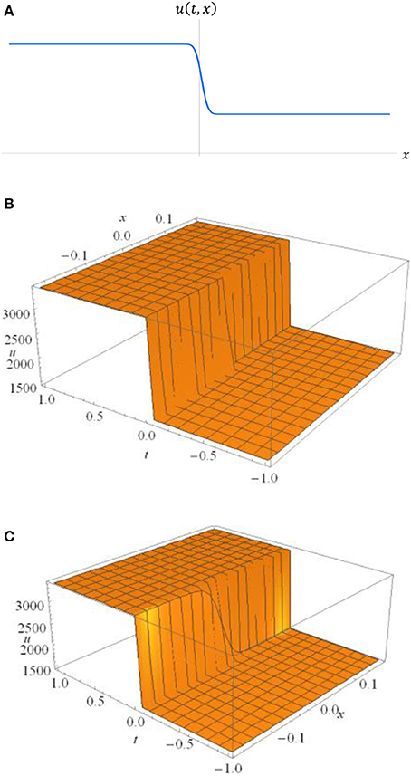
Figure 1. (A) Shock-wave solution illustrating the discontinuity between the incoming (horizontal) wave velocity of u (t, x) = v_I = 3, 415 m/s, and the outgoing velocity of u (t, x) = v_F = 1461.794 m/s—where v_I and v_F are each taken to be constant for −∞ ≤ x ≤ 0 and 0 ≤ x ≤ ∞, in this case, respectively. In the case of a spatially fixed-size skull, there are actually three intervals, whereby −∞ ≤ x ≤ 0, 0 ≤ x ≤ x_R and x_R ≤ x ≤ ∞, each representing v_I = 3, 415 m/s, v_F = 14671.794 m/s and then v_I = 3, 415 m/s again, respectively. Note that, in this graph, the vertical-axis represents general (non-linear) velocity, u (t, x), whilst the horizontal-axis generally represents distance, x meters. (B). Shock-wave solution, with a vanishingly-small diffusion coefficient, in 3-dimensions over the spatio-temporal ranges of −0.176 ≤ x ≤ 0.176 m and −1 ≤ t ≤ 1 s. If the solution is plotted with x and t axes reversed, Mathematica simply rotates the plot by 90°. As characteristic of plotting all shock-waves, its motion is essentially illustrated as propagating with respect to both the x- and t-axes, with a sharp discontinuity at x = 0 and t = 0, primarily. (C) Shock-Wave solution, with a moderately-small diffusion coefficient, in 3-dimensions over the spatio-temporal ranges of −0.176 ≤ x ≤ 0.176 m and −1 ≤ t ≤ 1 s. As in (B), if the solution is plotted with x and t-axes reversed, Mathematica simply rotates the plot by 90°. As is characteristic of the plotting of all shock-waves its motion is, again, essentially illustrated as propagating with respect to both the x- and t-axes.

Taking this explanation further, it is hoped that the smoothing term of Burgers' equation could potentially be applied—within more practical contexts—to mitigate against both initial shock- and resulting pressure-wave within an actual combat situation, for example. Certainly, graphically speaking, when γu_xx is applied to the original first-order Burgers' equation—Equation (3)—one can clearly see that the shock-wave becomes considerably (and necessarily) smoothed out, as illustrated in Figure 1C. It should be obvious—from the three-dimensional graphical plots—that this factor has had considerable effect in greatly reducing the severity of the shock, within a purely mathematical context.

Given this mathematical and physical evidence, it may be conjectured that such theoretical calculations, and the clear negative damping effects to this extent, will eventually be the basis for a technology that will ultimately mitigate not only against initial transitory IED shock-waves, but also against resulting, equally harmful, pressure-waves that occur immediately thereafter, either within the brain, or on the battlefield.

In the following models from the literature, the solutions to the associated PDEs—such as the Burgers' and Transport equations, especially involving calculated variable pressures—will illustrate just how significant (within the context of mathematical models at this stage) this smoothing term is, in greatly reducing high-magnitude pressures (often in terms of Mega- or Giga-Pascals) to nothing more than mere fractions. These will sometimes be in the order of one millionth of a Pascal, or smaller, above and below the base-level of atmospheric standard temperature and pressure (STP), the latter taken to be that of zero Pascals.

One should be aware, given the experimentally-observed, calculated (experimentally or theoretically) and graphically-plotted pressure curves where the pressure generally tends to repeatedly vary between negative and positive values, and similarly for pressure-gradients of the same respective signs, that they are generally not referred to as monotonic functions. Instead, they are more likely to be oscillatory in nature—or at least may contain oscillatory frequencies within an exponentially decaying curve itself, at least—where respective functions also display varying opposite signs and varying first derivatives, as suggested by the analysis of both reflection and transmission coefficients in the section Preliminary Mathematical Exposition: Effect of the Directional Nature of Shock-Waves on Reflection and Transmission Coefficients, Resulting Pressure-wave and Energies, Related to Conservation Laws and the Rankine-Hugoniot Jump Condition. It is this oscillatory nature of pressure-waves that sets them apart from the often monotonically decreasing or increasing functions that generally describe initial shock-waves in the theoretical sense, as profiled in Figures 1A–C, 2 (though the latter can also illustrate oscillatory motion as well, under certain circumstances). These are facts a researcher should be aware of, certainly in terms of mathematically modeling both types of observed results—for example, when an individual intends to apply Fourier analysis to transform a discrete curve (or discrete data) into its representative continuous form. In these terms, oscillatory—and therefore periodic—solutions have been sought for the pressure-models, in several cases in this paper, in order to describe and explain the varying pressures observed experimentally. Fourier analysis should also bear fruit in this respect.

FIGURE 2

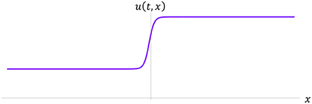
Figure 2. Rarefaction-wave solution illustrating the discontinuity between incoming (horizontal) wave velocity of u (t, x) = v_I = 1461.794 m/s and outgoing velocity of u (t, x) = v_F = 3, 415 m/s—where v_I and v_F are each taken to be constant for −∞ ≤ x ≤ 0 and 0 ≤ x ≤ ∞, in this case, respectively. For the case of a spatially fixed-size skull there are, again, three separate intervals, whereby one writes, −∞ ≤ x ≤ 0, 0 ≤ x ≤ x_R and x_R ≤ x ≤ ∞, each representing v_I = 1461.794 m/s, v_F = 3, 415 m/s and then v_I = 1461.794 m/s again, respectively. Note, in this graph, the vertical-axis represents general (non–linear) velocity, u (t, x), and the horizontal–axis generally represents distance, x meters.

It is worth noting, at this point, that the brain mass-diffusivity coefficient, γ, of the one-dimensional Laplacian, u_xx, as is well known in neurological literature, is often vanishingly small, having the dimensions of square meters per second. This results in the product of these two factors, known as the smoothing term, γu_xx, displaying the dimensions of acceleration, or meters per second squared (as might be expected) —a potentially important factor both significant and vital later in this paper's analysis. This assumes that we first consider pressure as the ratio of force to area, as will be explained and illustrated. Figures 1A,C illustrate shock-wave solutions for at least two values of γ, and (Figure 1B) describes a shock with a much smaller diffusivity coefficient as opposed to that of Figure 1C.

A series of further suggestions, including re–direction of the wave, would also use existing knowledge of wave mechanics, such as: absorption, reflection, refraction, diffraction, polarization, dispersion and the final technique of interference—the latter particularly utilizing the application of superposition to cancel out the waves (the converse of which enhances them in size and amplitude). The adoption of such principles within a more practical context, also taking into consideration the wave's phase (including possible application of the above smoothing term), would inevitably be highly beneficial in many ways.

The Mathematical Model and Its Analysis

We first define the velocity of the shock-wave as u (t, x), which propagates over the spatial-interval (diameter of the brain), 0 ≤ x ≤ 0.176 m [1], and over an interval of time defined as the period, 0 ≤ t ≤ T s, for some value of t.

We can apply the chain-rule to u (t, x), in order to arrive at the following quasi–linear Burgers' equation although, since it is a well-known PDE, it is stated here for brevity, which is:

$\begin{array}{cc}\begin{array}{r}\frac{\partial u}{\partial t}+u\frac{\partial u}{\partial x}=\gamma \frac{{\partial }^{2}u}{\partial x^2}\end{array}& (15)\end{array}$

or otherwise depicted as:

$\begin{array}{cc}\begin{array}{r}{u}_t+u{u}_x=\gamma u_{xx}\end{array}& (16)\end{array}$

When γ is vanishingly small, either of these two equations reduce to the first-order form, as follows:

$\begin{array}{cc}\begin{array}{r}{u}_t+u{u}_x=0\end{array}& (17)\end{array}$

Equation (17) is very similar to the following Equation (18), in which the weakly non-linear term, u, transforms into its linear version, c (a constant velocity), such that we now have:

$\begin{array}{cc}\begin{array}{r}{u}_t+c{u}_x=0\end{array}& (18)\end{array}$

Equation (18) is known as the Transport equation, or linear Burgers' equation, and most forms of the above PDEs will be used in the analysis below, when and where necessary. In addition, one should also note that it is possible for u to be a function of x only, such that u = c(x), in some situations. This should be taken into consideration when applying the respective models.

Burgers' Equation Derivation in Terms of Velocity and Pressure—A Simplified Result of the Navier–Stokes Equation

Since pressure is equal to force per unit area, and assuming incompressibility of brain tissue, we can make the assumption that pressure, in the case of a shock-wave, can be written as:

$\begin{array}{cc}\begin{array}{l}{P}_1=\frac{F}{A}=\frac{m}{A}\stackrel{·}{U}=\frac{m}{A}(u_t+u{u}_x)\hfill \end{array}& (19)\end{array}$

where the sum of u_t and uu_x is simply the overall acceleration, $\dot{U}$, expressed as such, not only due to requiring correct units and dimensions, but because it is necessary to write the equation in this form for a shock-wave propagating with respect to both the t − x axes. The analogy is that of both radial- and transverse- velocity (and acceleration) within the discipline of Newtonian Celestial Mechanics.

Given that the left-hand-side of Equation (19) can also be expressed in terms of the smoothing-term, γu_xx, otherwise known as the Laplacian—having exactly the same dimensions as the expression on the right-hand-side, u_t + uu_x–then we have the second-order version, given by:

$\begin{array}{cc}\begin{array}{r}{P}_2=\frac{m\gamma }{A}{u}_{xx}\end{array}& (20)\end{array}$

Note that u_xx is the second partial derivative of the velocity, u, the latter being the partial derivative of x, which means that u_xx–representing the third partial derivative of x—does not represent acceleration, unlike the additive terms on the right-hand-side of Equation (19).

In many neurological contexts, when the pressures, P₁ and P₂, are required to be the same, Equations (19) and (20) may be equated to yield the original Burgers' Equation (16), in which the common factor m/A then simply cancels completely—thus leaving the mass-diffusivity coefficient, γ, on the right-hand-side of the PDE, including the remaining partial derivatives on both sides. Therefore, as expected, we have the Burgers' equation once again:

$\begin{array}{l}{u}_t+u{u}_x=\gamma u_{xx}\end{array}$

This identical result to Equation (16) further suggests that Burgers' equation is the most appropriate model, at this stage, to employ—to model neurological shock- and pressure-waves, as explained in the next paragraph. It is also noteworthy here that both Equations (19) and (20) in their individual forms will be vital, later on, for modeling the two types of pressure-wave according to each of these respective equations. This is especially so for mathematically applying the smoothing term in Equation (20), to vastly reduce the otherwise enormous pressures.

In terms of the significance of Burgers' equation, the author concludes that it can be applied for purposes of mathematical calculation—and for modeling of (especially) the non-linear variation in neurological pressure. Merely postulating its potential relevance and use to this effect is further supported by its being a simplification of the incompressible Navier-Stokes' equation:

$\begin{array}{cc}\begin{array}{r}\frac{\partial u}{\partial t}+(u\nabla )u-\gamma {\nabla }^{2}u=\nabla P+g\end{array}& (21)\end{array}$

In the above equation, Equation (21), $\frac{\partial u}{\partial t}$ represents the variation of u with respect to increasing time; (u∇)u represents the time-independent acceleration of flow (of the shock, with velocity u) with respect to space (or more simply, the convection); the Laplacian term, γ∇²u, is the diffusion (or acceleration of that diffusion with respect to spatial coordinates), perhaps more accurately described as the diffusion momentum of the fluid viscosity, determined by the diffusion coefficient, γ. The first term on the right-hand-side of the equals sign, ∇P, often known as the internal source, is simply a pressure gradient, otherwise described as the time-independent rate of change of pressure with respect to the spatial coordinate, x, whilst the final term, g, is simply an external source.

Although proof and use of the Burgers' equation—Equation (16) —to model neurological pressure–waves was independently verified above, the terms ∇P and g were not initially considered. It is perhaps fortunate that their inclusion at this point was formerly neglected, partly for ease and simplicity of calculation. Furthermore, the external source, g, can be neglected, unless one finds it advantageous to model factors occurring outside the skull and brain. The resultant equation, therefore, which is as follows:

$\begin{array}{cc}\begin{array}{r}\nabla P=\frac{\partial u}{\partial t}+(u\nabla )u-\gamma {\nabla }^{2}u\end{array}& (22)\end{array}$

is either a positive or a negative resultant pressure gradient, ∇P. It is also the case that, according to both the Divergence Theorem and Green's Theorem for conservative (vector) fields—both of which are related—this pressure gradient, ∇P, is sometimes equal to zero. The mathematical modeling of this result has already been achieved in Mathematica, and will be discussed later. However, one should point out that the explanation of Equation (22) has important consequences, not only to model pressure, but also with regard to energy considerations and other factors.

Now that we have established at least one correct equation to use in the following model for both shock and pressure-waves, we need to determine appropriate boundary conditions (BCs), before these equations are solved and appropriately plotted using Mathematica software.

Boundary Conditions for a Typical Case

A General Shock-Wave (or Compression-Wave) Solution

For the current mathematical-model in a real-life simulation of a shockwave entering the skull-bone from the atmosphere, before propagating through the brain, exiting at the opposite side, then traveling onwards and outwards indefinitely, we take data from the literature [1].

It is necessary to note that initial pressure-wave speed, c_p, of 3415 m/s through the skull-bone, as modeled by Mediavilla et al. [1], is assumed to be constant. However, on reaching the initial skull–brain interface, there is an almost instantaneous and discontinuous drop in this velocity to 1461.794 m/s (the value having been re–calculated, from their own experimental data, for greater accuracy). This is one of the factors determining the non-linearity of the system, the shock being due to the Rankine-Hugoniot jump-condition relating to the conservation laws, viz., the conservation of mass, energy, and momentum.

The Mathematica plots, employed throughout this paper, indicate that this latter initial velocity of 1461.794 m/s then increases non–linearly as the wave propagates through the brain tissue, as Mediavilla et al. [1] confirmed on measuring the velocity increasing to 1463.415 m/s at a distance of 0.03 m to the next sensor. At the final distance of 0.176 m, at the opposite brain-skull interface—using the conservation laws—the velocity instantaneously jumps back up to its original value of 3, 415 m/s once more, energy transfer issues being ignored here. It travels through the skull-bone once again, and exits the head as described above—though the Mathematica plots do not specifically show this physical feature, largely for analytical reasons.

The Mathematica simulation also indicates that there is still some variability in this velocity, in terms of it increasing non-uniformly to a higher value than that of 1461.794 m/s, before then rapidly increasing to the final higher velocity of 3,415 m/s (again due to the conservation laws [10]) in the final stage of transit, as Mediavilla et al. [1] confirmed. Most mathematical shock-wave simulations do consider these two initial and final (Rankine-Hugoniot) velocities of the wave to be constant over the relevant intervals, especially for simplicity of calculation, as illustrated in Figure 1A.

Rarefaction-Waves (or Expansion-Waves)

It is also necessary to point out that, if the velocity magnitudes (or speeds) had been reversed in the above general shock-solution, such that v_I = 1461.794 m/s and v_F = 3, 415 m/s, over the same intervals, then we would have a special case of a solution; this would be known as a rarefaction (or expansion) wave, as illustrated in Figure 2.

The nature of a rarefaction-wave is that, over a given spatial interval, in this case, 0 ≤ x ≤ 0.176 m, the gradient being $u(t,x)=\frac{dx}{dt}$, each characteristic curve describing a shock-wave's propagation (as plotted with respect to the t − x axes) dissipates with increasing time. A more detailed explanation of this motion can be seen by solving Equations (17) and (18) via the method of characteristics. One of the simplest examples of such a solution is the linear case, resulting in straight lines “fanning-out” with respect to the t − x axes as time, t, increases indefinitely vs. the given, fixed diameter, x, of the brain. A general solution to Equations (17) or (18) can be shown to yield an expression in the form:

$\begin{array}{cc}\begin{array}{r}u(t,x)=\frac{{\alpha }_{1}x+{\beta }_1}{{\alpha }_{2}t+{\beta }_2}\end{array}& (23)\end{array}$

where α₁, β₁, α₂, and β₂ are constant coefficients. One can see that for each particular-solution, as t increases indefinitely over the region 0 ≤ x ≤ x_R, where $t>-\frac{\beta }{\alpha }$, the limiting value of u(t, x) is:

$\begin{array}{cc}\begin{array}{l}\underset{t\to \infty }{\text{lim}}\left\{u\left(t,x\right)\right\}=\underset{t\to \infty }{\text{lim}}\left\{u\left(t,L\right)\right\}=\underset{t\to \infty }{\text{lim}}\left\{\frac{x_R}{\alpha t+\beta }\right\}\\ =\underset{t\to \infty }{\text{lim}}\left\{\frac{L}{\alpha t+\beta }\right\}=0\end{array}& (24)\end{array}$

From the above analysis, we can see that the velocity, u (t, x), becomes negligible with increasing time, t, for each characteristic curve, and therefore approaches the value of zero m/s when x is equal to the fixed and relatively small, finite value of L. In many cases, u (t, x) can even change magnitude and direction, depending upon evolutionary conditions within the situation, thus assuming a negative value. One could ascertain this from the slope of such characteristics, certainly within a theoretical sense, but also physically, particularly when the shock-wave induces the resulting, reflected pressure-wave, for example. This is especially true when considering the limiting value of u (t, x) as t → −∞, although this is perhaps impractical and unrealistic, except analytically. In addition, if the constant, β, is calculated to be negative, such that αt−β < 0, or αt < β, then the velocity will again be negative. One can also verify that, when $t=-\frac{\beta }{\alpha }$, such that α t + β = 0 (where u (t, x) is undefined), one witnesses an inherent discontinuity, as in the case of the initial shock-wave solution described in the section General Shock-Wave (or Compression-Wave) Solution.

One may infer that, given a range of velocities describing the same propagating shock—especially when considering the resulting reflected pressure-wave, where negative velocities are indeed apparent—then a change in velocity from positive to negative value, or vice versa [through a stationary state, u (t, x) = 0], for example, has an equally damaging effect due to this motion. One harmful effect of this continually reflected pressure-wave, and therefore its resulting oscillatory behavior, is that it actually causes a reduction in the existing normal neurological pressure. The consequences of such reductions in this pressure are that the lower-than-average values are scientifically measured in terms of negative quantities. This effect in many cases results in an observable presence of cavitation [14], a process whereby liquids boil at lower temperatures, given their presence in lower-than-average pressure environments. This effect is a process allowing the molecules of a fluid to escape, usually from the surface, when the surrounding atmospheric pressure is reduced to below normal levels. This could also result in the equally harmful effects of mTBI—in tandem with equally damaging effects of very high velocities and pressures [14].

The fact that the shock-wave velocity is so variable, throughout its spatio-temporal journey, to the extent that resulting pressure-waves even switch signs (due to reflection and continually rebounding inside the skull, from wall-to-wall) and direction, is precisely why the whole science of shock-wave dynamics is said to be non-linear, as opposed to the linearity of constant velocity. This is why shock-waves are described and explained by the above non-linear PDEs, and Burgers' equation in particular, especially within a neurological context, as in any other.

As mentioned above, the variation in both positive and negative velocities and pressures, due to reflection of the incident shock-wave within the skull–brain configuration, leads to the conclusion that resulting propagation of such a pressure-wave is not only oscillatory but also potentially periodic. The presence of these factors leads one to assume that a choice of periodic boundary-conditions is often more suitable to model this type of behavior. Accordingly, some of these functions will now be adopted below.

In addition to the above, for the purposes of this particular model, and in the case of either non-linear shock- or rarefaction-waves (and precisely because of this non-linearity), one needs to find a sufficient function that satisfies, or yields, the two values of the function, |u(t, x)|_L = v_I and |u(t, x)|_R = v_F, at both initial and final boundaries (given either of the values for t or x, or even a combination of both).

Also, only a function that varies according to this non-linearity will suffice for any model, so it is very necessary to ensure that an appropriate function satisfying the given boundary conditions is deduced, as we then require this suitably chosen function to successfully derive both general and particular-solutions. This should ultimately predict the resulting motion, as accurately as possible, within a reasonable degree of error. However, achieving mathematical perfection, in terms of precisely modeling observations of experimentation in this regard, may leave something to be desired, given the multitude of complex factors involved in nature itself.

Partially due to the damping of the resulting oscillatory behavior of the waves—as experimentally observed—a number of different models containing boundary conditions of both exponential and sinusoidal natures may be adopted in the initial stages. It is also possible to choose other more complicated functions where necessary, including hyperbolic functions, as may occasionally be required.

Thus, combinations of the elementary exponential functions of form e^ax and e^bt and the trigonometric functions of form sin (ωx) and cos (ωt), such as e^ax sin (ωx) and e^bt cos (ωt)–even perhaps involving both independent variables, t and x, simultaneously—will often satisfy the modeling of damped IED shock-wave dynamics, certainly for the purposes of this paper.

Determining General Boundary Conditions for Each Case

In the above section, the boundary conditions that were suggested as appropriate functions to use in this particular set of models, as dictated by existing literature, can be deduced, then applied to the general solution of Burgers' equation: Equation (17).

To initially model the resulting neurological shock-waves with Mathematica, the PDEs that best describe the mechanics are—as highlighted above—Equations (16) and (17):

$\begin{array}{l}{u}_t+u{u}_x=\gamma u_{xx}\end{array}$

and:

$\begin{array}{l}{u}_t+u{u}_x=0\end{array}$

for which the average brain mass-diffusivity coefficient, γ, in Equation (2), is so vanishingly small, roughly equal to 1 × 10⁻⁹m²/s, that it has been neglected in Equation (3), for modeling the human brain, in the first instance.

Each of the above Equations (16) and (17) are relatively elementary to solve (in the absence of initial conditions), but Equation (17) is perhaps easier to adopt for modeling both the initial shock-wave and resulting pressure-wave, given that it represents the actual discontinuous shock-wave in contrast to the continuous solution described by Equation (16). Indeed, Equation (17) is in the form:

$\begin{array}{cc}\begin{array}{r}a(t,x)u_t+b(t,x)u_x=c(t,x)\end{array}& (25)\end{array}$

whereby, in this case:

$\begin{array}{l}a(t,x)=1,b(t,x)=u(t,x)=u,andc(t,x)=0\end{array}$

To solve (17), and then seek to run the resulting shock-wave simulation in Mathematica, we reduce it (as is normal for this type of parabolic PDE), to the set of three ordinary differential equations (ODEs) representing the characteristic lines of slope for the system, written as:

$\begin{array}{cc}\begin{array}{r}\frac{dt}{a(t,x)}=\frac{dx}{b(t,x)}=\frac{du}{c(t,x)}\end{array}& (26)\end{array}$

Equations (25) and (26), which describe the solution to every single point on the surface of the shock–wave, are fairly elementary to prove but, for the purposes of this model, we find the general solution in the first instance.

Thus, we write Equation (26) as follows, performing the usual methods of integration. Henceforth, we have:

$\begin{array}{cc}\{\begin{array}{c}\frac{dx}{b(t,x)}=\frac{du}{c(t,x)}\\ \frac{dt}{a(t,x)}=\frac{du}{c(t,x)}\end{array}& (27)\end{array}$

Due to a, b and c being constants, in this case, then each of these two ODEs in equation (27) are separable, therefore yielding:

$\begin{array}{cc}\{\begin{array}{c}b{{\displaystyle \int }}^{}du=c{{\displaystyle \int }}^{}dx\\ a{{\displaystyle \int }}^{}du=c{{\displaystyle \int }}^{}dt\end{array}& (28)\end{array}$

On solving each of these equations in Equation (28), where the first yields a function of x, and the second a function of t, the solutions are written as:

$\begin{array}{cc}\{\begin{array}{c}u={\alpha }_{1}x+A(k)\\ u={\alpha }_{2}t+A(k)\end{array}& (29)\end{array}$

The next step is to determine the third solution to Equation (26), obtained by writing:

$\begin{array}{l}\frac{dt}{a}=\frac{dx}{b}\end{array}$

which yields:

$\begin{array}{cc}\begin{array}{r}x=A(k)t+k\end{array}& (30)\end{array}$

such that the constant of integration, k, can now be expressed as:

$\begin{array}{cc}\begin{array}{r}k=x-A(k)t\end{array}& (31)\end{array}$

before substitution into A (k) to obtain a solution of u (t, x) = u (x − A (k) t).

Preamble to the Cauchy Problem

In the section Determining General Boundary Conditions in Each Case, the latter characteristic solution is at least one of two well-known methods for solving both Burgers' and the Transport equations—apart from several other methods, at least—allowing for the deduction of a minimum of one solution as outlined in Equation (29), especially when the situation being considered is an initial-boundary-value problem. There are infinitely many solutions for the Transport equation, depending on the choice of the velocity-gradient, c, and the value of the intercept, k, along with the intersection of each characteristic with another for a different velocity, c, resulting in a shock at the relevant point, (t, x)–so no individual curve in this situation is unique.

Each of the methods referred to above utilizes the general method of characteristics, and the second—in addition—makes close reference to the Cauchy Problem, therefore resulting in a pair of equations for both t and x–along with expressions representing other combinations of relevant parameters, such as k. This can usually be solved simultaneously in order to facilitate a more appropriate expression for u (t, x) as accurately as possible, where necessary. This is particularly true when dealing with these types of parabolic PDEs, especially when the situation requires an initial-boundary value problem approach.

In such models as these, which include most of the PDE problems throughout this paper, the characteristic method of solution has largely been adopted, particularly to model shock-wave solutions wherever necessary. As will be discussed in this latter section, a slightly more convoluted—but necessary—method has been implemented, in which an extra dummy-variable, s, or k (as stated above), has been introduced to obtain the highest degree of precision available that the model requires.

In order to solve this type of problem effectively, one must apply the Cauchy Problem, as stated in definition 1 below. If this problem is applicable, as it is for the purposes of this research, then it will greatly assist the determination of at least one solution.

In the non-linear problem, expounded in the section Boundary Conditions Within a Typical Case, it turns out that the combined solution of the two equations in Equation (29) yields an implicit function of k. This means that the resulting function cannot easily be solved explicitly for k, without employing further analytic methods. This indicates that the Cauchy Problem is ideal in finding a solution, since both of the composite functions that have been adopted as a model can be expanded as a composite series, the Cauchy Problem specifically requiring such a feature.

For example, in such a situation, one expands the initial boundary condition, u (x) = u (k), ideally as a spatially-based series in the form of $u(k)=a_0+a_{1}x+a_2{x}^2+\dots +a_n{x}^n$ and then the limit of this as k approaches zero is determined. This process enables one to separate out the necessary variables, to obtain an expression for k in the usual manner. Adopting this method should result in a satisfactory solution for u(t, x), once the eventual expression for k has been re-substituted into the original function, u(k). As the graphical-curves imply within this section, the models that follow this procedure appear to indicate the experimental observations.

The Use of the Cauchy Problem to Determine More Appropriate Spatial Boundary Conditions for the Shock-Wave Solution

Definition 1: The Cauchy Problem

For a partial differential equation that defines a surface, S ∈ ℝⁿ, for n = {1, 2, …}, then the Cauchy Problem specifies that if both an initial analytic function, ϕ (0, x) = ϕ(x), and its normal derivative, $\frac{\partial \varphi }{\partial x}={\varphi }_x(x)$, exist within the neighborhood of point (t₀, x₀), for both the initial conditions, t = t₀ and x = x₀, and where the boundary conditions can be expanded and defined by the series:

$\begin{array}{l}\varphi (x)=a_0+a_{1}x+a_2{x}^2+\dots +a_m{x}^m\end{array}$

where a_i ∈ ℝ, for i = {0, 1, 2, …, m}, making it possible to differentiate this function:

$\begin{array}{l}\frac{\partial \varphi }{\partial x}={\varphi }_x(x)\end{array}$

then this results in both a unique and reasonably applicable solution, a procedure known as the Cauchy problem.

An Appropriate Boundary Condition Leading to a Characteristic Solution in the Case of a Shock-Wave

Following on from the section Use of the Cauchy Problem to Determine More Appropriate Spatial Boundary Conditions for Shock-wave Solution, since c (t, x) = 0 in the above equations—Equation (28) in this particular case—then each is effectively identical, either simultaneously yielding the integral:

$\begin{array}{cc}\begin{array}{r}{\displaystyle \int }du=0\end{array}& (32)\end{array}$

to which the solution, again, for both of them, is:

$\begin{array}{cc}\begin{array}{r}u=A(k)\end{array}& (33)\end{array}$

Here, u is a “quasi–constant,” or a currently unknown function of k, the latter being, as yet, the undetermined characteristic equation, written in terms of independent variables, t and x.

The third ODE from (26), above, is:

$\begin{array}{cc}\begin{array}{r}\frac{dt}{a(t,x)}=\frac{dx}{b(t,x)}\end{array}& (34)\end{array}$

or, since a(t, x) = 1 and b(t, x) = u = A(k), we have:

$\begin{array}{cc}\begin{array}{r}{\displaystyle \int }dx=A(k){\displaystyle \int }dt\end{array}& (35)\end{array}$

or

$\begin{array}{cc}\begin{array}{r}x=A(k)t+k\end{array}& (36)\end{array}$

Normally, if one knew the identity of function, A (k), which satisfies the boundary conditions at this stage, one would substitute it into Equation (33) and thus determine the time at which the shock will occur by partially differentiating each side of it, with respect to k. A basic linear boundary condition of the form A (k) = αk +β, in which k is a characteristic curve, a function of t and x itself, will return general solutions in the form of both Equations (29) and (33), respectively, dependent upon the given parameters.

We do not need to differentiate Equation (33) immediately, at this stage, but need a boundary condition representing a shock-wave solution, certainly at either end of the range 0 ≤ x ≤ 0.176 m, and one not only plotting a more accurate graph of the wave-like nature of this phenomenon, but one resulting in a reasonable particular-solution for shock–wave velocity, u (t, x), over the range of x itself. It is again not only practical, but mathematically required, as outlined in definition 1 in the section Use of the Cauchy Problem to Determine More Appropriate Spatial Boundary Conditions for Shock-wave Solution, to choose a boundary condition only including the variable x–chosen because the boundary condition must also be analytic at t = 0, and ideally not undefined. In other words, one must be able to write the boundary condition as a function of x, and x only, such that a solution exists within the neighborhood of the point (t₀, x₀).

Once we obtain the velocity, u (t, x), after first applying the method of characteristics, we shall be able to compare this result with the solution for u (t, x), obtained via perhaps the more well-known method of substituting u (t, x) = v (x − ct) for a wave propagating with velocity, c, from the left–hand–limit, measured at x = 0 m, toward the right–hand–limit, measured at x = 0.176 m, over the diameter of the brain. This second method, utilizing the smoothing term as discussed in the section Burgers Equation Derivation in Terms of Velocity and Pressure—Simplified Result of Navier-Stokes Equation', may be outlined within any future papers when discussing continuity of the solution and mitigation against the shock-wave's jump–discontinuity, in which one obtains the solution:

$\begin{array}{cc}\begin{array}{r}u(t,x)=\frac{\alpha +\beta e^{-\frac{(\beta -\alpha )(x-ct-\delta )}{2\gamma }}}{1+e^{-\frac{(\beta -\alpha )(x-ct-\delta )}{2\gamma }}}\end{array}& (37)\end{array}$

or, whereby the often vanishingly small term, δ, can be neglected, we have:

$\begin{array}{cc}\begin{array}{r}u(t,x)=\frac{\alpha +\beta e^{-\frac{(\beta -\alpha )(x-ct)}{2\gamma }}}{1+e^{-\frac{(\beta -\alpha )(x-ct)}{2\gamma }}}\end{array}& (38)\end{array}$

where α and β are constants of integration.

The three-dimensional shock-wave plots for Equation (38) are illustrated in Figures 1B,C, in the section Rarefaction-Waves (or Expansion-Waves), above. The first of these Figures 1B, represents a shock-discontinuity for a very acute and vanishingly small diffusivity coefficient, γ ≪ 1, in other words, when γ ≅ 0, and the second (Figure 1C), represents a more moderate discontinuity when 0≪ γ < 1. The latter of these two graphs also indicates the type of smoother solution that is normally to be expected when the smoothing term itself, γ u_xx, is applied to the right-hand-side of Equation (17), being part of its purpose. This mathematical feature of Burgers' equation is partially responsible for the earlier suggestion that one could potentially apply it upon the battle-field, assuming suitable technology is developed to be utilized effectively.

Addendum 1

It is important to note here that we define u (t, x) in the form of:

$\begin{array}{l}u(t,x)=v\left(\frac{x}{c}-t\right)\end{array}$

since we are particularly interested in determining the nature of a shock-wave, u (t, x), propagating with respect to the temporal axis, t, where $\frac{x}{c}$ is measured in units of time (usually in seconds), rather than the spatial axis defined by:

$\begin{array}{l}u(t,x)=v(x-ct)\end{array}$

which is measured in meters.

Hence the difference in these Galilean relativistic transformations of the respective coordinates.

Decreasing Sinusoidal Function, Obeying Boundary Conditions of the Propagating Shock, as Well as the Resulting Pressure-Wave

From the collection of graphs of pressure vs. time, in Figure 9 of the paper written by Moore et al. [2], it is evident that a given sinusoidal function, or at least an appropriate decreasing sinusoidal function representing a negatively damped system, may be applicable to model the propagating shock–wave. This theoretical assumption was outlined in the section Preliminary Mathematical Exposition: Effect of the Directional Nature of Shock-waves on Reflection and Transmission Coefficients, Resulting Pressure-wave and Energies, Related to Conservation Laws and the Rankine-Hugoniot Jump Condition above, and after referral to the literature, for example [15].

In many of the plotted graphs that were produced within the above-cited literature, it appears they bear a striking similarity to oscillatory motion and, therefore, periodic, wave-like motion of the form of exponentially-decaying sinusoids, such as basic trigonometric functions, sin (ωx) and cos (ωx), each combined with the exponential functions e^−ωx and e^−x.

Appropriate Use of Various Forms of Decreasing Sinusoidal Boundary Conditions

In order to model many of the observational experiments of neurological shock-waves, such as those conducted by Mediavilla et al. [1], there is a good case for applying exponentially decaying sinusoidal pressure-waves in the form of e^−ωx sin (ωx) and e^−x sin (ωx), each obeying the Cauchy Problem in the section Use of the Cauchy Problem to Determine More Appropriate Spatial Boundary Conditions for Shock-wave Solution. Either of these functions can be used to model the observed physics, but the literature itself initially indicated that it was not clear why both negative and positive pressure-gradients, including over- and under- pressures, seemed to occur on separate occasions and under differing experimental conditions.

The above fact can be explained by the phase angle at which the shock-wave enters the brain, a factor determined by the underlying physics—such as the initial conditions. “In such cases whereby an angular phase–difference is apparent, so one also obtains either a negative or positive pressure-gradient. For example, in different physical situations, it is necessary to deduce that one or the other of the above functions will be more appropriate, or possibly both.”

In the case of a complementary phase difference, the sinusoidal function $sin(\frac{\pi }{2}-\omega x)$ is equated to cos(ωx), in the simplest case, and vice versa for $cos(\frac{\pi }{2}-\omega x)$. This is a little more complex for non-complementary phase differences, such as cos (ϕ − ωx), in which case other trigonometrical identities, such as the double angle formulae, are required when $\varphi {\ne }^{\pi }{/}_2$. The current Mathematica models used for this analysis have either assumed complementary identities for initial simplicity or, by using the initial conditions, a different angular value, ω, has been determined for both sin (ωx) and cos (ωx), respectively, with further modifications.

Thus, depending upon the physical situation in hand, either one or the other of the above decaying functions will more appropriately model the observed result in many cases, but one's preference about which is more applicable, and as to which of them also models the situation more accurately, is largely determined by the underlying physics, the initial conditions, and one's own educated guesswork!

Elementary Model for Pressure-Wave With Simple Undamped Sinusoidal Function, Obeying Cosine Boundary Conditions

In the first instance of graphing an appropriate shock–wave solution, where v_I > v_F, along with its particular-solution, as in Figure 1 above, an initial boundary condition can be written as:

$\begin{array}{cc}\begin{array}{r}u(x)=v_I\mathrm{\text{cos}}(\omega x)\end{array}& (39)\end{array}$

in which v_I represents the initial incident shock–wave velocity, and x is the fixed–variable spatial–coordinate (in one–dimension, for simplicity), indicating the diameter of the brain. The constant of proportionality, ω radians, is the frequency of the propagating wave over the brain's diameter. It is possible to vary ω, according to the concept of the fundamental frequency, to determine a sinusoidal function more accurately describing any shock–wave's unique physical characteristics—dependent upon all the given parameters involved. The final, outgoing velocity of the shock-wave is taken to be u (t, L) = v_F, and the above expression in Equation (34) must satisfy each of the two boundary conditions dictating that u (t, 0) = u (0) = u₀ = v_I, and u (t, L) = u (L) = u_L = v_F, respectively—otherwise Equation (36) would fail to model the situation appropriately or accurately.

Borrowing the observed numerical data from Mediavilla et al. [1], during one part of their experiment, in which v_I = 3, 415 m/s and v_F = 1461.794 m/s, one now inserts each of these values into Equation (39), thus yielding:

$\begin{array}{cc}\begin{array}{r}3415\mathrm{\text{cos}}(\omega x)=1461.794\end{array}& (40)\end{array}$

Since $x=0.176=\frac{176}{1,000}$ m, and ω is a currently unknown parameter, we are able to conclude, via elementary calculation, that ω ≅ 6.412 radians. Therefore, one possible boundary condition is:

$\begin{array}{cc}\begin{array}{r}u(x)=3415\mathrm{\text{cos}}(6.412x)\end{array}& (41)\end{array}$

Since the fundamental frequency, f = nω, also allows the function to obey the boundary conditions, where n = 0, 1, 2, 3…, we may write Equation (41) in the modified form:

$\begin{array}{cc}\begin{array}{r}u(x)=3415\mathrm{\text{cos}}(n\omega x)\end{array}& (42)\end{array}$

or,

$\begin{array}{cc}\begin{array}{r}u(x)=3415\mathrm{\text{cos}}(6.412nx)\end{array}& (43)\end{array}$

for = 0, 1, 2, 3….

In order to determine and plot the particular-solution for the given shock–wave over the given range of 0 ≤ x ≤ 0.176, one is required to substitute some expression satisfying the initial boundary conditions into Equation (33).

We note that in Equation (33), the quasi-constant, A(k), is present, and we now need to express this as an appropriate function in terms of both x and t, by first deducing the currently unknown characteristic equation, k. Since we are aware, from Equation (33), that:

$\begin{array}{l}u=A(k)\end{array}$

then, using Equations (39)–(43) for a first solution, we may write:

$\begin{array}{cc}\begin{array}{r}A(k)=3415\mathrm{\text{cos}}(\omega k)\end{array}& (44)\end{array}$

On substituting the more general form of Equation (44), for simplicity and generality, into Equation (36), we then obtain:

$\begin{array}{cc}\begin{array}{r}x=v_I\mathrm{\text{cos}}(\omega k)t+k\end{array}& (45)\end{array}$

The procedure, now, is to make k the subject of Equation (45), but this is somewhat problematic, since k is implicit. However, if the appropriate analytical procedures are applied to the cosine term, which can be expressed as an infinite sequence of terms, one deduces that, for the required small values of ωk, we have:

$\begin{array}{l}{\displaystyle \underset{k\to 0}{lim}}\left\{cos(\omega k)\right\}=1\end{array}$

such that:

$\begin{array}{cc}\begin{array}{r}x=at+k\end{array}& (46)\end{array}$

in which powers greater than or equal to terms in k² have been neglected.

Equation (46) can be rearranged to yield:

$\begin{array}{cc}\begin{array}{r}k=x-at\end{array}& (47)\end{array}$

On substituting Equation (47) into Equation (44), we therefore obtain one possible approximate particular-solution, written as:

$\begin{array}{cc}\begin{array}{r}u(t,x)=v_{I}cos\omega (x-at)\end{array}& (48)\end{array}$

whereby, in this case, v_I = 3415 m/s and ω ≅ 6.412. Since Equation (48) is now expressed in terms of both spatio-temporal coordinates, x and t, one may be able to observe more easily that it has been necessary to replace A (k) with u (t, x) in Equation (36), above, to obtain Equation (48). A Mathematica plot of the shock–wave solution, using Equation (48), is shown below in Figures 3A,B. Also, plots of the same solution, using boundary conditions as defined by Equation (39), are shown more fittingly in Figures 4, 5.

FIGURE 3

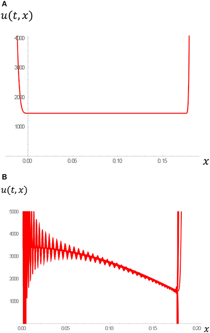
Figure 3. (A) Sinusoidal shock-wave solution for Equation (34), for the appropriate frequency ω≅6.412, satisfying the required boundary conditions of the shock-wave of velocity, u (t, x), over the fixed spatial-interval 0 ≤ x ≤ 0.176 m up to a time period of 1 s. (B) Sinusoidal solution of Equation (42), with ω≅6.412, of a shock-wave solution curve, with velocity u(t, x), over the fixed spatial interval 0 ≤ x ≤ 0.176 m up to a time period of 1 s. Note that the transitory shock-wave's minimum velocity within this model is 1461.794 m/s, and does not actually reduce to zero, nor becomes negative in value, as this oscillatory graphical-plot appears to suggest for a larger spatial-range. This solution indicates the sinusoidal nature of the type of function chosen, resulting in two shock-discontinuities at x = 0 and x = 0.176 m over the given spatial-range, described perhaps more clearly in (A) (Figures 4, 5).

FIGURE 4

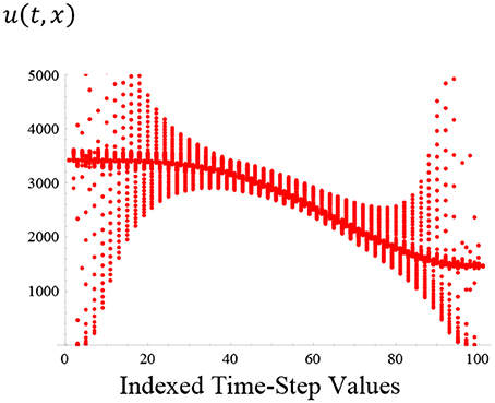
Figure 4. A similar sinusoidal solution to that illustrated in Figure 3A, again with frequency ω≅6.412, of the shock-wave of velocity, u (t, x), this time shown to propagate with respect to the indexed time-step values up to 1 s at the 100th position (or the 100th point on the graph). A sharper graph may be obtained by reducing not only the time-period, but also the time-step and the count for this scenario.

FIGURE 5

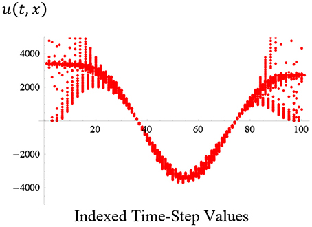
Figure 5. Another exemplary sinusoidal solution, this time with increased frequency increased to ω≅32.06, of the shock-wave of velocity, u (t, x), again shown propagating with respect to the indexed time-step values up to 1 s at the 100th position (or the 100th point on the graph). A sharper graph may be obtained by reducing not only the time-period, but also the time-step and the count for this scenario.

Note that in in Figures 4, 5, the shock–wave solution bears some resemblance to the more idealized graphical plot of Figure 1, except that, due to the nature of the initial boundary condition used in this section, along with the resulting particular-solution, the sharpness of the discontinuity that would otherwise be observed has been smoothed out, due to the cosine term.

Unlike the solution illustrated in Figures 1A–C, where there is an apparently instantaneous drop in velocity from u (t, x) = v_I to the lower value of u (t, x) = v_F at around x = 0 (the latter of which then continues on its journey, indefinitely, at this latter value), the apparent velocity reversal in Figure 5, can still be suitably explained, by way of applying the relevant mechanics to the nature of the oscillating variation in pressure, again with respect to both spatio–temporal variables, x and t.

As mentioned earlier, and based upon cited literature, the reflection of the pressure within the skull-brain cavity—as described by Figure 5—results in positive and negative values of u (t, x), largely due to the pressure's oscillatory behavior, and as indicated by the sinusoidal functions adopted as explanations for these occurrences.

The alternative Mathematica plot of velocity, u (t, x), vs. time, t–as calculated by Mathematica, and with fixed spatial coordinate, x, also suppressed—is shown in the discrete-curves plot, Figure 5, below.

On analysis of Figure 5, one notices that it is not quite as characteristic of the typical shock-wave propagating through the brain, as previously illustrated in Figures 1A–C,3A,4. This is largely due to the sinusoidal nature of the plotted curves, involving an artificially induced frequency of ω ≅ 32.06, passing through zero velocity and then becoming negative—which seems to indicate u (t, x) reversing direction in such a case.

Conclusion

Within this paper, essentially modeling the physics of neurological shock-waves in the human brain due to IEDs, the groundwork has been laid out in preparation for more involved development of the material in any future work.

In particular, it has been established, via initial analysis of both conservation laws and reflection coefficients in the section Preliminary Mathematical Exposition: Effect of the Directional Nature of Shock-waves on Reflection and Transmission Coefficients, Resulting Pressure-wave and Energies, Related to Conservation Laws and the Rankine-Hugoniot Jump Condition, that the incident shock-wave results in damped, oscillatory, motion of the resulting shock- and pressure- wave profiles. Each of these single factors, taken together, therefore support the application of the Burgers' equation model, together with exponentially-decaying sinusoidal boundary conditions, in order to describe the initial shock-wave—otherwise known as a compression-wave—and the resulting physics that takes place within the human head, both during and after immediate impact.

Due to the asymmetry of the human head, and consistent with historic and existing shock-tube experiments, only a one-dimensional model has been adopted here to simplify calculation.

As stated earlier, from analysis of the reflection coefficients, it is also realized that the ensuing physics within the system yields rebounding waves continually illustrating velocities oscillating back and forth—as illustrated in the above plots. The subsequent negatively-valued velocity reversals in the diagrams lend to the additional notion of the existence of rarefaction—meaning that the gases (or at least the media) within the brain then (similarly) violently expand—shortly after the initial shock-wave has occurred. This factor is believed to yield a number of neurological conditions, including damage to the brain's DNA, particularly resulting from cavitation [7], due to the ensuing lower than normal neurological pressure, when the cerebral fluids begin to boil more freely due to neurological pressure dropping below its normal base-level.

That significant velocity reversals and cavitation [7], are both witnessed indicate the occurrence of a significant difference in pressure between the point of impact and at some point in the future. It is reasonable to assume that one is able to apply the same Burgers' equation to model the resulting pressure-profile, post-shock. As described above, this is achieved by applying exponential-decaying sinusoidal boundary coefficients, resulting in very interesting graphical plots, each bearing a significant likeness to the Friedlander curve [16–19], together with under-pressures describing the presence of cavitation.

It is intended that this part of the analysis will be dealt with in future work.

Author Contributions

The author confirms being the sole contributor of this work and approved it for publication.

Conflict of Interest Statement

The author declares that the research was conducted in the absence of any commercial or financial relationships that could be construed as a potential conflict of interest.

References

1. Mediavilla VJ, Philippens M, Meijer SR, van den Berg AC, Sibma PC, van Bree JLMJ, et al. Physics of IED blast shock tube simulations for mTBI research. Front Neurol. (2011) 2:58. doi: 10.3389/fneur.2011.00058

CrossRef Full Text | Google Scholar

2. Moore DF, Jérusalem A, Nyein M, Noels L, Jaffee MS, Radovitzky RA. Computational biology – modeling of primary blast effects on the central nervous system. Neuroimage (2009) 47(Suppl. 2), T10–20. doi: 10.1016/j.neuroimage.2009.02.019

PubMed Abstract | CrossRef Full Text | Google Scholar

3. Cernak I. Blast-induced neurotrauma models and their requirements. Front Neurol. (2014) 5:128. doi: 10.3389/fneur.2014.00128

PubMed Abstract | CrossRef Full Text | Google Scholar

4. Needham CE, Ritzel D, Rule GT. Wiri suthee, young leanne. Blast testing issues and TBI: experimental models that lead to wrong conclusions. Front Neurol. (2015) 6:72. doi: 10.3389/fneur.2015.00072

CrossRef Full Text

5. Risling M. Blast induced brain injuries – a grand challenge in TBI research. Front. Neurol. (2010) 1:1. doi: 10.3389/fneur.2010.00001

PubMed Abstract | CrossRef Full Text | Google Scholar

6. Moss WC, King MJ, Blackman EG. Skull flexure from blast waves: a mechanism for brain injury with implications for helmet design. Phys Rev Lett. (2009) 103:108702. doi: 10.1103/PhysRevLett.103.108702

PubMed Abstract | CrossRef Full Text | Google Scholar

7. Taylor PA, Ford Corey C. Simulation of blast-induced early-time intracranial wave physics leading to traumatic brain injury. J Biomech Eng. (2009). 131:061007. doi: 10.1115/1.3118765

PubMed Abstract | CrossRef Full Text | Google Scholar

8. Grujicic M, Bell WC, Pandurangan B, He T. Blast-wave impact-mitigation capability of polyurea when used as helmet suspension-pad material. Mater Des. (2010) 31, 4050–4065. doi: 10.1016/j.matdes.2010.05.002

CrossRef Full Text | Google Scholar

9. Kovacs SK, Leonessa F, Ling GSF. Blast TBI models, neuropathology, and implications for seizure risk. Front Neurol. (2014) 5:47. doi: 10.3389/fneur.2014.00047

PubMed Abstract | CrossRef Full Text | Google Scholar

10. Olver PJ. Introduction to Partial Differential Equations (2014). Springer.

Google Scholar

11. Gerber N. Note on Shock Reflection Coefficient. Ballistic Research Laboratories, Aberdeen Proving Ground, Maryland. Memorandum Report No. 1775 (1966).

12. Chen Y, Constantini S. Caveats for using shock tube in blast-induced traumatic brain injury research. Front Neurol. (2013) 4:117. doi: 10.3389/fneur.2013.00117

PubMed Abstract | CrossRef Full Text | Google Scholar

13. Chafi MS, Karami G, Ziejewski M. Numerical analysis of blast-induced wave propagation using FSI and ALE multi-material formulations. Int J Impact Eng. (2009) 36:1269–75. doi: 10.1016/j.ijimpeng.2009.03.007

CrossRef Full Text | Google Scholar

14. Cao Y, Risling M, Malm E, Sondén A, Bolling MF, Sköld MK. Cellular high-energy cavitation trauma – description of a novel in vitro trauma model in three different cell types. Front Neurol. (2016) 7:10. doi: 10.3389/fneur.2016.00010

PubMed Abstract | CrossRef Full Text | Google Scholar

15. Miller K, Chinzei K, Orssengo G, Bednarz P. Mechanical properties of brain tissue in vivo: experiment and computer simulation. J Biomech. (2000) 33:1369–76. doi: 10.1016/S0021-9290(00)00120-2

PubMed Abstract | CrossRef Full Text | Google Scholar

16. Friedlander FG. The Diffraction of Sound Pulses I. Diffraction by a Semi-Infinite Plane Royal Society. Communicated by G. I. Taylor (1940). Available online at: http://rspa.royalsocietypublishing.org/

17. Friedlander FG. The Diffraction of Sound Pulses II. Diffraction by an Infinite Wedge Royal Society. Communicated by G. I. Taylor (1940).

18. Friedlander FG. The Diffraction of Sound Pulses III. Note on an Integral Occurring in the Theory of Diffraction by a Semi-Infinite Screen. Royal Society. Communicated by G. I. Taylor (1941).

19. Friedlander FG. The diffraction of sound pulses IV. On a paradox in the theory of reflexion. Proc R Soc A Math Phys Sci. (1946) 186:356–67. doi: 10.1098/rspa.1946.0049

CrossRef Full Text | Google Scholar