Persistent Entrainment in Non-linear Neural Networks With Memory

Introduction

Brain stimulation has become increasingly popular in neuroscience to support a wide variety of experimental and clinical interventions [1–4], being used to guide and/or entrain populations of neurons with periodic electromagnetic signals. In many experiments, outlasting responses exceeding the duration of the stimulation period have raised much attention. Many studies have shown that following rhythmic stimulation, altered neuronal synchrony can be measured for periods lasting from seconds to hours after stimulation [5]. Such transient responses have been suggested to support some of the reported physiological and cognitive changes triggered by stimulation [6] and much efforts have been deployed to stabilize stimulation-induced alterations in brain dynamics. More recently, periodic stimulation has been used to entrain brain oscillations for extended periods of time, in which neural synchrony remains locked to the stimulation frequency even after it has been turned off in a state dependent way [7, 8]. However, it remains unclear how such rhythmic stimulation combines with the endogenous oscillatory brain activity to produce the observed aftereffects. Various mechanisms such as reverberation [9], multistability [10], and synaptic plasticity [11] have been suggested as mediators of these effects.

To better understand this phenomenon, we consider a network of neural populations with delayed feedback implementing a particular type of dynamic memory. Such delayed feedback systems appear not only in neural system but also in optics [12, 13], regulatory networks [14], postural and mechanical control [15], as well as electronic logic gates [16]. We use this type of model to study the effect of periodic forcing on neural activity, especially transient responses observed after forcing offset. We investigate how persistent entrainment arises and how it relates to the time delay and the intensity of the noise driving the populations. Our analysis shows that periodic forcing can selectively excite intrinsic oscillatory modes that are part of the system's reservoir of resonances, and provoke damped oscillatory perturbations that outlast the forcing time. In doing so, we also present a novel analysis of resonant forcing phenomenon in a delayed feedback network, a topic that has only received limited attention in contrast to non-delayed dynamical systems (see e.g., [17] for a study of resonances in the context of chemotherapy for delayed hematological dynamics). We use mean-field theory and linear stability analysis to quantify the sensitivity of our network to forcing frequency and the duration of persistent oscillations that go on after the stimulation has been removed. We propose to capitalize on this mechanism to optimize the effect of rhythmic stimulation and amplify post-stimulation effects.

Model

In the present work, we analyze the dynamics of a network of globally (i.e., all-to-all) interacting inhibitory neural populations whose membrane potentials u_i(t) evolve according to the following set of non-linear differential equations

$\begin{array}{ll}{s}^{-1}\frac{d}{dt}{u}_i(t)& =-u_i(t)+N^{-1}{\displaystyle \sum _{j=1}^N}{w}_{ij}f\left[u_j(t-\tau )\right]+S(t)\\ +\sqrt{2D}{\xi }_i(t)\hfill & (1)\end{array}$

where s = 10 ms is the membrane time constant and where τ is a variable mean conduction delay. The network schematic is illustrated in Figure 1. The firing rate function f has a non-linear sigmoid shape and is defined by $f\left[u_i\right]={(1+exp\left[-\beta u_i\right])}^{-1}$. The synaptic weights w_ij are such that < w_ij >_NxN = g, where g is the mean synaptic strength. In the present work, we assume a network of inhibitory populations, and thus w_ij < 0 for all i, j. The activity of individual populations is perturbed by recurrent input, independent Gaussian white noise ξ_i of intensity D and periodic forcing S(t) = S cos(ωt) that drives all nodes equally. With the set of parameters chosen, the network exhibits slow non-linear oscillations as depicted in Figure 1B. The intensity of the noise controls the amplitude of the limit cycle oscillations by tuning the stability of the asynchronous state. For low values of noise intensity D, the network stabilizes into strong non-linear oscillations, but when noise increases, synchronous oscillations in Equation (1) are gradually suppressed and the network becomes asynchronous. This relationship between internal noise and oscillatory activity is in line with the task-dependent desynchronization observed in cortical populations during sensory processing and movement [e.g., [18]].

FIGURE 1

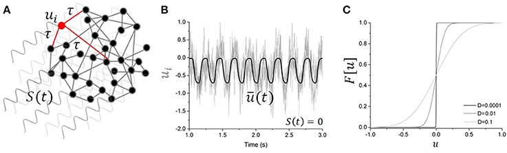
Figure 1. Driven nonlinear network model. (A) Schematic illustration of the network with global periodic forcing S(t) driving the activity of N recurrently connected units with time delay τ. One unit is highlighted in red, with local connections (only a limited set are shown). (B) Activity of the individual nodes (light gray lines) in absence of forcing (i.e., S(t) = 0) for the network governed in Equation (1). The mean network activity $\overline{u}(t)$ is also plotted (bold line), showing that the network parameters are such that the network exhibits an endogenous oscillation. Here τ = 200 ms, g = −3, D = 0.1, and s = 10 ms. (C) Effective non-linear response function changes as noise intensity increases. Increasing D linearizes the response function.

Whenever noise in the system is sufficiently small (i.e., D ≪1) one may express the dynamics of individual nodes in Equation (1) as fluctuations around a network average $\overline{u}(t)$ i.e.,

$\begin{array}{ll}{u}_i(t)=\overline{u}(t)+{\nu }_i(t)& (2)\end{array}$

where the local fluctuations ν_i obey the Langevin equation

$\begin{array}{ll}{s}^{-1}\frac{d}{dt}{v}_i(t)=-v_i(t)+\sqrt{2D}{\xi }_i(t)& (3)\end{array}$

In this regime, we may easily derive the mean-field representation of the network dynamics in presence of global periodic forcing and independent noise sources. The mean field is given by the scalar non-linear delay-differential equation [19, 20]

$\begin{array}{ll}\frac{d}{dt}\overline{u}(t)=-\overline{u}(t)+gF\left[\overline{u}(t-\tau )\right]+S(t)& (4)\end{array}$

with the noise-corrected response function $F\left[u\right]=\frac{1}{2}\left(1+erf\left[\frac{u}{\sqrt{}(2D)}\right]\right)$ derived under the limit of large β, as seen in Figure 1C [20]. The mean field description in Equation (4) is a delayed oscillator with periodic forcing that represents the collective evolution of a network of neural populations and has been used to study stochastic non-linear oscillations in recurrent networks [19, 20]. In the analysis that follows, we focus our attention on the dynamics in Equation (1) and investigate properties of persistent responses analytically using Equation (4) while varying stimulation parameters and noise intensity.

Persistent Entrainement and Buffering of Periodic Signals

In the presence of periodic forcing, Equation (1) exhibits frequency-selective and persistent entrainment: oscillatory forcing-induced responses, whose duration exceeds the delay τ, can be observed after the forcing offset and for which the dynamics differ significantly from the one seen in the autonomous regime (i.e., before the forcing onset). This form of forcing buffering allows fluctuations due to the forcing to outlast the stimulation application; in fact, the forcing is being transiently memorized by the system. An example of this persistent entrainment effect is shown in Figure 2. Prior to the forcing onset, Equation (1) displays slow, non-linear oscillations at a frequency of about 5 Hz. But after the forcing offset (i.e., in the post-forcing period) autonomous oscillations appear at frequencies close to the forcing frequency. This form of spectral multistability, in which post-forcing activity differs from pre-forcing activity, appears to be frequency-selective. Indeed, as shown in Figures 2A,C, slightly different forcing frequencies did not trigger the same degree of persistent entrainment. The persistence of these oscillations appears to be linked to intrinsic resonance. In Figure 2B, the persistent frequency (i.e., peak frequency of the persisting oscillations in the post-forcing period) is the same as the forcing frequency. In addition to the increased duration of the entrainment, the system's amplitude during forcing is significantly larger compared to the other frequencies presented (Figures 2A,C), suggesting the presence of a resonance. In addition, Figure 2C shows that once the forcing stops, not only does the system relaxes back to its baseline oscillatory state, but the system also displays additional damped oscillations at a frequency of 13 Hz corresponding to the resonant frequency seen in Figure 2B.

FIGURE 2

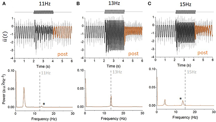
Figure 2. Example of persistent entrainment and sensitivity to stimulation frequency. (A) Activity in the network (Equation 1) before, during and after forcing is applied. The network mean activity (bold line) is shown alongside individual node responses (light gray lines). Before the forcing onset, the network displays synchronous oscillations of about 5 Hz. Sinusoidal forcing at a driving frequency of ω = 11 Hz is applied at t = 2 s for a duration of 2 s and stops afterwards. After forcing (orange line), the network mean activity relaxes back to its baseline oscillatory state rapidly. The bottom panel shows the power spectral density of the post-forcing activity (from which the mean was subtracted) for t within the interval (4, 6 s). A clear peak at 5 Hz can be seen, indicating that the system's response after forcing offset is dominated by its intrinsic, pre-forcing, frequency. (B) When periodic forcing with a frequency of ω = 13 Hz is applied, the response amplitude is significantly increased. After the forcing offset however, the system displays persistent entrainment at the forcing frequency: the network activity is dominated by 13 Hz oscillations that lasts for a period far exceeding the system time delay τ. This can also be seen from the strong peak of the power spectral density at 13 Hz (bottom). (C) When the forcing frequency is increased to ω = 15 Hz, an intermediate form of persistent entrainment can be observed. The system's activity relaxes back to its pre-forcing state, but damped oscillations at 13 Hz (i.e., not 15 Hz) can be observed. This is also revealed in the power spectral density plot (bottom) where two peaks can be seen: one at 4 Hz (intrinsic frequency) and one at 13 Hz (*). In all cases, the model parameters are the same except for the stimulation frequency with τ = 100 ms: g = −3, D = 0.1, and s = 1.

Linear Stochastic Stability With Time Delay

To better understand the phenomenon observed in Figure 2B and how it relates to the system's parameters, we performed a thorough stability analysis and investigated the effect of delay and noise on the linear eigenmodes of Equation (4). In absence of stimulation (i.e., S(t) = 0) and for g < 0, this equation possesses a unique equilibrium ${\overline{u}}_o$ which satisfies the implicit relationship

$\begin{array}{ll}{\overline{u}}_o=gF\left[{\overline{u}}_o\right]& (5)\end{array}$

Stability of the equilibrium state u_o is determined by considering small fluctuations around the fixed point to obtain the linearized dynamics. The linearized dynamics for Equation (4) with S(t) = 0 are then written as:

$\begin{array}{ll}\frac{d}{dt}\overline{u}(t)=-\overline{u}(t)+R\overline{u}(t-\tau )& (6)\end{array}$

where $R=g{F}^{{}^{\prime }}\left[u_o\right]=\frac{g}{\sqrt{2\pi D}}exp\left[-\frac{{\overline{u}}_o^2}{2D}\right]$. Although the equation above is linear in terms of $\overline{u}$, it is non-linear with respect to the noise intensity D and fixed point ${\overline{u}}_o$. Using the ansatz $\overline{u}(t)=ũe^{\lambda t}$ | λ ∈ ℂ, Equation (6) can be expressed in the form λ = −1 + Re^−λτ, from which we obtain the typical transcendental characteristic equation that defines the eigenvalues λ of Equation (6) in presence of delay [21],

$\begin{array}{ll}\lambda =\frac{W(R\tau e^{\tau })}{\tau }-1& (7)\end{array}$

where W is the Lambert function. The roots λ_k = α_k + i ω_k| α_k = Re[λ_k] ∈ ℝ, ω_k = Im[λ_k] ∈ ℝ of the characteristic equation above form the spectrum Λ = {λ_k} of the mean-field in Eq. (4) and determine its linear stability. These eigenvalues correspond to branches of the Lambert function W_k, where k = 0, ±, 1, ±2, ..±∞ index pairs of roots with increasing order. Associated modes $v_k=C_k{e}^{{\lambda }_{k}t}$| C_k ∈ ℂ, λ_k ∈ Λ span the stable (S), center(C) and unstable(U) manifolds i.e., Λ = S ⊕ C ⊕ U. Solutions of Equation (1) possess the mode expansion [22],

$\begin{array}{ll}\overline{u}(t)={\displaystyle \sum _{k=-\infty }^{\infty }}{C}_k{e}^{{\lambda }_{k}t}={\displaystyle \sum _{k=-\infty }^{\infty }}{C}_k{e}^{{\alpha }_{k}t}{e}^{i{\omega }_{k}t}& (8)\end{array}$

In this framework, the solution $\overline{u}(t)$ consists of a superposition of infinitely many oscillatory modes with damping rate α_k and eigenfrequencies ω_k. Stable limit cycle solutions emerge whenever a supercritical Hopf bifurcation occurs for which a pair of critical eigenvalues cross the imaginary axis; that is, for ${{\lambda }_{k=o}\equiv \lambda }_c=\pm i{\omega }_c|{\omega }_c=\underset{k}{min}|{\omega }_k|$, so that the following equation is satisfied [23],

$\begin{array}{ll}i{\omega }_c=\frac{W_o(R_c\tau e^{\tau })}{\tau }-1& (9)\end{array}$

for some critical values of $R_c^o$ and for the chosen delay τ and ω_c. Here W_o is the zeroth-order Lambert function. The set of critical values $R_c^o$ and τ at the Hopf bifurcation (HB) in Equation (9) are plotted in Figure 3. We note that as noise intensity is increased beyond the HB, higher order eigenvalues may also cross the imaginary axis, satisfying for α_k = 0,

$\begin{array}{ll}i{\omega }_k=\frac{W_k(R_c^k\tau e^{\tau })}{\tau }-1& (10)\end{array}$

FIGURE 3

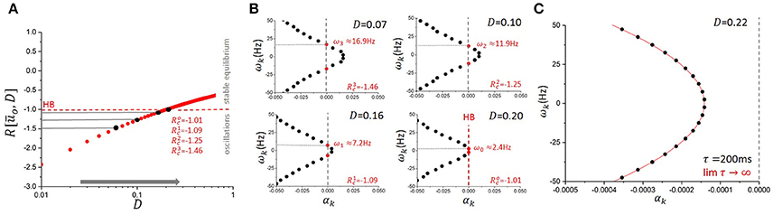
Figure 3. Effect of noise on system's stability and eigenmodes in the mean-field equation. (A) Increasing the amount of noise in the system (from left to right) effectively changes the shape of the response function in Equation (4). In the linearized system, this translates into an increase in the value of the linear gain R in Equation (6). Here, parameters in the model were chosen such that the network exhibits strong non-linear oscillations and thus increasing D linearizes the dynamics and pushes the system toward the fixed point on the other side of the Hopf bifurcation (HB, in red). (B) For lower values of D, eigenvalues where originally located on the right hand side of the imaginary axis. These modes were thus unstable with α_k > 0. Increasing D (from top left panel to bottom right) causes a successive passage of these eigenvalues toward the left hand side of the imaginary axis as the dynamics becomes more linear and the fixed point ${\overline{u}}_o$ recovers stability at the Hopf bifurcation (HB, in red). Through this process, noise can change the stability of individual eigenmodes and thus make specific eigenfrequencies more susceptible to persistent entrainment and consequentially, to buffering. Here τ = 200 ms. g = −1.5 and s = 1. (C) The asymptotic curve ${C}\left[\tau \right]=\left\{{\tau }^{-1}\gamma (\omega )+i\omega :\omega \in ℝ\right\}$ (red line) is plotted with numerically computed eigenvalues from Equation (7) (black markers) at τ = 200 ms. The other parameter values were set to g = −1.5, s = 1, D = 0.22 such that all eigenvalues lie on the left side of the imaginary axis. The plot demonstrates that with delay τ = 200 ms, the curve captures the distribution of the eigenvalues up to index k = 10 with minimal error.

The stability analysis above shows that in addition to the critical frequency ω_c observed near the HB in Equation (6), the set of eigenmodes in Equation (8) provide a reservoir Ω = {ω_k} of intrinsic resonances whose elements correspond to the imaginary parts of the eigenvalues λ_k of Equation (6). The analysis also shows that this set depends on noise intensity through the linear gain R. As such, changes in noise intensity D translate into variations in R which directly impact the stability of the system through changes in the elements of the spectrum Λ. The spectrum's elements gradually transit to the stable subspace. Such noise-induced changes in stability have been found to change bifurcation points [24] and alter the feature of delay-induced limit cycles [19, 25].

The effect of noise on the network eigenmodes and resonances can be seen in Figure 3 for a particular value of the time delay. While varying D, the system in Equation (4) can be set into distinct non-linear regimes characterized by a variable set of resonances. Each of these resonances reflect an excitation of oscillatory modes whose real part is in the vicinity or the right-hand side of the imaginary axis. The existence of these unstable eigenmodes defines the susceptibility of the network to persistent entrainment and mediates the outlasting responses observed in Figures 2B,C.

For large delays τ, the purely oscillatory eigenvalues λ = iω at the HB can be approximated as follows. The ansatz $\overline{u}(t)=ũe^{i\omega t}$ onto Equation (6) gives a system of equations pertaining to the real and imaginary components of $\overline{u}(t)$,

$\begin{array}{llll}{R}_c^{k}cos({\omega }_k\tau )& =& 1& (11)\end{array}$

$\begin{array}{llll}{R}_c^{k}sin({\omega }_k\tau )& =& \omega & (12)\end{array}$

Using the fact that as τ → ∞, ω_k → 0 [26] and $R_c^k<0$, Equation (11, 12) give the large delay approximation ${\omega }_k\cong \frac{(2k+1)\pi }{\tau }$. Furthermore, with large delays the eigenvalues of Λ are closely distributed along an analytic curve. Defining ${C}=\left\{\gamma (\omega )+i\omega :\omega \in ℝ\right\}$, where $\gamma (\omega )=-\frac{1}{2}log(\frac{1+{\omega }^2}{R^2})$, it follows that for each rescaled eigenvalue λ[τ] = ατ + iω, α + iω ∈ Λ, dist$({C},\lambda \left[\tau \right])\to 0$ as τ → ∞ [26]. That is, for sufficiently large delay, each eigenvalue λ∈Λ lies close to the curve ${C}\left[\tau \right]=\left\{{\tau }^{-1}\gamma (\omega )+i\omega :\omega \in ℝ\right\}$. Figure 3C graphically demonstrates this result by plotting an instance of numerically computed eigenvalues from Equation (6) with the rescaled curve ${C}\left[\tau \right]$. Combining this result with the large delay approximation for each eigenfrequency, we obtain a simple analytic approximation for each eigenvalue as ${\lambda }_k\cong {\tau }^{-1}\gamma ({\omega }_k)+i{\omega }_k,{\omega }_k=\frac{(2k+1)\pi }{\tau }.$

Resonance and Excitation of Oscillatory Eigenmodes

To understand the interaction between the forcing and the system's oscillatory modes, we can examine the particular solution in the linearized case in Equation (6) to reveal susceptibilities to persistent entrainment. The susceptibility to forcing of various frequencies can be characterized by computing the resonance curves of the periodically forced linear delayed system

$\begin{array}{ll}\frac{d}{dt}\overline{u}(t)=-\overline{u}(t)+R\overline{u}(t-\tau )+S(t)& (13)\end{array}$

where S(t) = Scos(ωt). To reveal resonances, we simply consider the ansatz,

$\begin{array}{ll}\overline{u}(t)=A(\omega )sin(\omega t)+B(\omega )cos(\omega t)& (14)\end{array}$

Substituting this into Equation (13) and solving for the amplitudes A(ω) and B(ω), one can easily compute the amplitude of the solutions $\overline{u}$ as

$\begin{array}{ll}\parallel \overline{u}\parallel =\sqrt{A{(\omega )}^2+B{(\omega )}^2}& (15)\end{array}$

Where

$\begin{array}{ll}A(\omega )=-\frac{cos(\omega \tau )R-1}{(R^2+2sin(\omega \tau )R\tau -2cos(\omega \tau )R+1+{\omega }^2)}& (16)\end{array}$

and

$\begin{array}{ll}B(\omega )=-S\frac{sin(\omega \tau )R+\omega }{(R^2+2sin(\omega \tau )R\tau -2cos(2\omega \tau )R+1+{\omega }^2)}& (17)\end{array}$

Inserting Equations (16, 17) into Equation (14) yields the desired resonance curve

$\begin{array}{l}\parallel \overline{u}\parallel =\frac{S}{\sqrt{-2sin(\omega \tau )R\omega -{\omega }^2+2cos(\omega \tau )R-R^2-1}}\\ =\frac{S}{\sqrt{Re{\left[{Q}(R,\tau ,\omega )\right]}^2+Im{\left[{Q}(R,\tau ,\omega )\right]}^2}}& (18)\end{array}$

where

$\begin{array}{ll}{Q}(R,\tau ,\omega )=i\omega +1+R{e}^{i\omega \tau }& (19)\end{array}$

which is just the characteristic equation of Equation (6) evaluated at the forcing frequency ω. The amplitudes of the solutions thus diverge here whenever a pair of imaginary eigenvalues cross the imaginary axis. Resonance curves are shown in Figure 4, where the amplitude $\parallel \overline{u}\parallel$ of oscillatory solutions of the linearized system are plotted as a function of the noise intensity and forcing frequency. As the delay is increased, one can see that the density of resonant frequencies increases; this is related to the behavior of the density of modes for the autonomous system [27]. Solution amplitudes increase and then diverge when the associated pair of eigenvalues cross the imaginary axis.

FIGURE 4

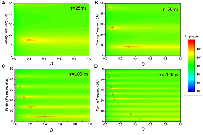
Figure 4. Resonance curves with variable delays and noise values for the linearized system in Equation (11). The system possesses a reservoir of resonances, corresponding to peaks in the amplitude of forced solutions. As noise in increased, the linear gain R changes and eigenmodes (whose frequencies are highlighted by the dashed lines) sequentially cross the imaginary axis, leading to a sequence of divergent linear modes (gray circles). The density of resonant frequencies—the number of peaks per unit frequency—increases with time delay. Aside from the divergences observed at the critical points, the relative amplitude of slower frequencies increases as noise increases: slow eigenmodes become prevalent while faster ones are damped, as seen from the passage of eigenvalues toward the left hand side of the imaginary axis in Figure 3. The delays used were: (A) τ = 25 ms; (B) τ = 50 ms; (C) τ = 100ms; and (D) τ = 200 ms. Here g = −1.5 and s = 1.

The linear analysis above tells us that in Equation (15), forced solutions possess a resonance for all eigenfrequencies ω_k. However, it remains unclear how these resonances relate to one another with respect to persistent activity. Figure 4 shows that the resonance peak amplitude varies as a function of noise, suggesting that specific frequencies have greater amplitude than others when it comes to transient activity. Note the tendency of the different mode frequencies to line up with harmonics of the fundamental network frequency ω_o as the delay increases [27]. To understand how persistent entrainment scales with forcing frequency, we chose a given noise intensity and examined the duration of persistent responses in Equation (1) while exciting individual modes with forcing frequencies aligned with those computed in Equation (10) on the basis of the linear stability analysis. The results are shown in Figure 5, where one sees that the system possesses a reservoir of resonances that can be individually excited to induce outlasting responses. The square wave limit cycle solution seen prior to forcing onset characterizes the oscillatory response of system with large delays [13]. These results show that the duration of persistent entrainment is inversely proportional to forcing frequency: slower frequencies produce more persistent effects. This result highlights the difference between the linear and non-linear cases. Linear stability predicts, through resonance curves computed in Equation (18) that the amplitude of forced solution is proportional to the proximity to the imaginary axis, a fact that is quite clear in Figure 4. However, Figure 5 shows that eigenvalues situated far to the right from the imaginary axis causes more persistent responses.

FIGURE 5

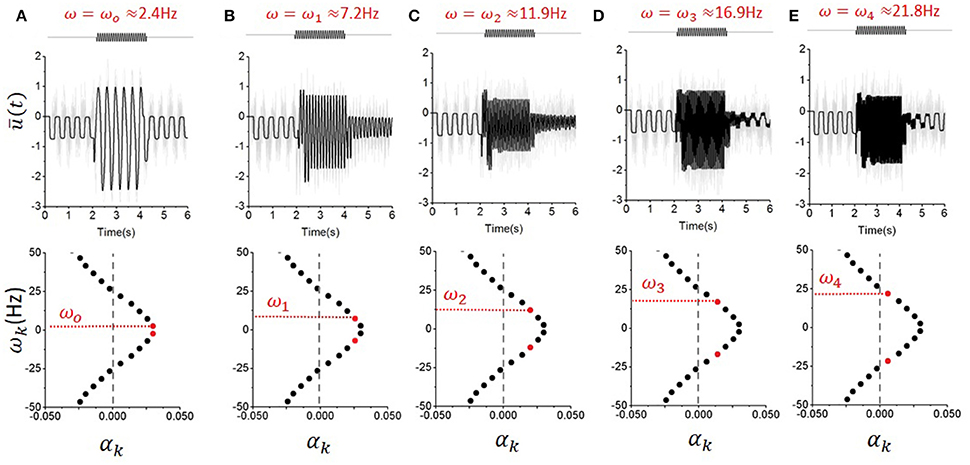
Figure 5. Persistent entrainment mediated by the selective excitation of unstable eigenmodes. Here, the noise intensity is set such that the first five eigenvalues are located to the right hand side of the imaginary axis. Then, forcing with frequency ω aligned with the eigenfrequencies ω_o−4 is successively applied. One can see that the amplitude of the response during forcing is not monotonically changing with forcing frequency, suggesting the presence of non-linear resonances that arise from the coupling of the linear modes by the system's nonlinearities. Persistent entrainment can be observed in every case, but its duration decreases with forcing frequency. The frequencies used were: (A) ω = 2.4 Hz; (B) ω = 7.2 Hz; (C) ω = 11.9 Hz; (D) ω = 16.9 Hz; (E) ω = 21.8 Hz; Here, D = 0.1, τ = 200 ms, g = −1.5 and s = 1.

To better characterize how the amplitude of persistent responses change as a function of forcing frequency, we numerically computed the power spectral density of persistent responses (after forcing offset) for all pairs of values of noise intensity and forcing frequency in the mean-field model given by Equation (4). We then computed the peak power at the forcing frequency during that period. Results are shown in Figure 6. The amplitude of persistent responses is larger for slower frequencies. This is in line with what is shown in Figure 5. We note that this scaling is also seen in Figure 4D for larger values of noise and beyond the HB (i.e., for values of noise exceeding the divergence associated with the dominant critical mode). We also computed in Figure 6B the frequency associated with persistent responses (after forcing offset) for the same set of parameters. Buffering occurs through a restricted set of output frequencies; independently of the forcing frequency ω, persistent entrainment is observed at one of the system intrinsic frequencies ω_k.

FIGURE 6

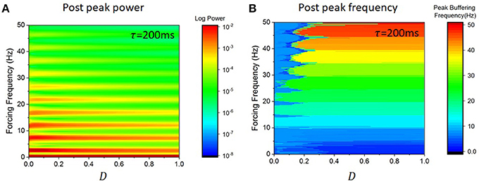
Figure 6. Persistent entrainment power and frequency as a function of forcing parameters in the mean-field equation in Equation (4). (A) Power measured at the forcing frequency after forcing offset as noise intensity is changed. Power is inversely proportional to forcing frequency. Only forcing frequencies aligned with the linear eigenfrequencies displayed significant power. (B) Peak frequency of the persistent responses as a function of noise intensity and forcing frequency. One can see that only a discrete set of frequencies can be expressed by the system, leading to a sequence of plateaus corresponding to the eigenfrequencies. The width of these plateaus is fixed and does not vary for higher noise intensities, indicating that the system with exhibit persistent responses at the closest eigenfrequency closest to the forcing frequencies. Here again τ = 200 ms, g = −1.5 and s = 1.

Buffering Duration

We note that despite their persistence, persistent responses are not stable orbits. Rather, the system's activity will always relax back to the oscillation defined by the dominant bifurcating eigenvalues (i.e., the poles, responsible for the autonomous dynamics before forcing onset). As seen in Figure 5, the convergence time appears to depend on forcing frequency. The speed at which excited resonances converge back to the autonomous oscillation can be thought of as a measure of persistence; but this is difficult to quantify given that according to linear stability, the associated eigenmodes are unstable (i.e., α_k > 0) and thus solutions diverge. We may nonetheless obtain an estimate of the entrainment duration using an approximation based on the superposition of damped oscillations. Without loss of generality, let us consider the case where the mean activity in Equation (13) under the absence of stimulation (i.e., S(t) = 0) is given by a supersposition of eigenmodes

$\begin{array}{ll}\overline{u}(t)\approx {\displaystyle \sum _{k=-\infty }^{\infty }}{C}_k{e}^{{\alpha }_{k}t}{e}^{i{\omega }_{k}t}={\displaystyle \sum _{k=-\infty }^{\infty }}{\overline{u}}_k(t)& (20)\end{array}$

The principal eigenvalue λ_o ≡ λ_c = α_c + iω_c defines the dominant oscillatory mode of the system and also corresponds to the eigenmode for which α_c > α_k and ω_c < ω_k | ∀k ≠ 0 and λ_k ∈ Λ. As such, we may rewrite the solution as

$\begin{array}{cc}\begin{array}{l}\overline{u}(t)\approx e^{{\alpha }_{c}t}\left(C_c{e}^{i{\omega }_{c}t}+{\displaystyle \sum _{k=-\infty ,k\ne 0}^{\infty }{C}_k{e}^{\left({\alpha }_k-{\alpha }_c\right)t}{e}^{i{\omega }_{k}t}}\right)=\overline{U}\hfill \end{array}\left(t\right)e^{{\alpha }_{c}t}& (21)\end{array}$

We may consider Equation (21) as an oscillator $\overline{U}(t)$ modulated by an exponentially growing envelope $e^{{\alpha }_{c}t}$. Let us now consider $\overline{U}(t)$: given that α_k − α_c < 0, taking the limit as t > +∞ yields linear asymptotic dynamics of the system without forcing,

$\begin{array}{ll}\overline{U}(t)\approx C_c{e}^{i{\omega }_{c}t}& (22)\end{array}$

We assume that a forcing S(t) = Scos(ω_kt) is applied with a frequency aligned with one of the system's eigenfrequencies and for a sufficiently long period of time. One may thus approximate the activity of an excited mode once forcing is removed as,

$\begin{array}{cc}\begin{array}{l}\overline{u}(t)\approx e^{{\alpha }_{c}t}\left(C_c{e}^{i{\omega }_{c}t}+K\left(s\right)C_k{e}^{\left({\alpha }_k-{\alpha }_c\right)t}{e}^{i{\omega }_{k}t}\right)\hfill \end{array}& (23)\end{array}$

for some constant K(S). As such, the oscillatory perturbation is induced by the forcing at an effective damping rate of α_k − α_c and thus at a characteristic damping time that we define as the buffering time: an estimate of the persistence of the excited mode ${\overline{u}}_k$. It is defined by

$\begin{array}{ll}{\delta }_k=\frac{1}{|{\alpha }_k-{\alpha }_c|}\approx \frac{\tau }{Re\left[|W_k(-R\tau e^{-\tau })-W_o(-R_c\tau e^{-\tau })|\right]}& (24)\end{array}$

According to this approximation, buffering time decreases as forcing frequency increases. We also note that the critical eigenvalue k = c has an infinite buffering time, which is consistent since the limit cycle with frequency ω_c is stable. The dependence of the buffering time on the time delay and linear gain is shown in Figure 7. As one can see, the persistence duration decreases as the eigenfrequency increases. This is analogous to what is seen in Figure 5. One can also see that Figure 7 further confirms the delay plays a crucial role in defining the decay rate of the persistent oscillations.

FIGURE 7

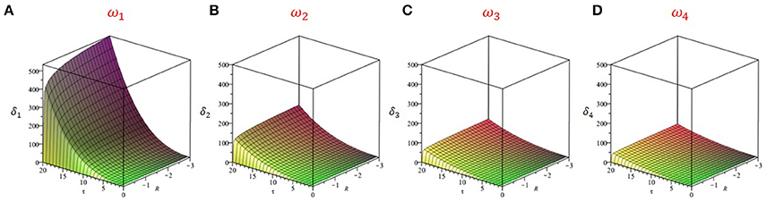
Figure 7. Buffering time δ as a function of the delay τ and linear gain R for the first four eigenmodes. We used the linearized system in Equation (6) and computed buffering times as per Equation (22). The buffering time associated with the zeroth order mode i.e., ω_o = ω_c is infinite and thus only the next four modes are shown i.e., k = 1, 2, 3, and 4. The duration of persistent responses decreases as the eigenfrequency increases. The frequencies used were: (A) ω₁ = 7.2 Hz; (B) ω₂ = 12.0 Hz; (C) ω₃ = 16.9 Hz; (D) ω₄ = 21.7 Hz. The delay is the dominant control parameter of buffering time: longer delays are responsible for more persistent responses. Note that these panels are related to the excited modes in Figures 5B–E, but for different delays. Here g = −1.5 and s = 1.

Multiple Stimulation Frequencies

We have also numerically investigated the response of the mean-field in Equation (4) to forcing with multiple frequencies to see whether persistent entrainment could carry multiple resonances—not only one. We have here considered the case a dual-frequency stimulation i.e., S(t) = S₁cos(ω₁t) + S₂ cos(ω₂t), where ω₁ and ω₂ were chosen to be eigenfrequencies of Equation (4). As shown in Figure 8, stimulation at a combination of eigenfrequencies appears to lead to persistent responses displaying a mixture of damped modes. Here again, the square-wave oscillations are a signature of large delays [13]. We can presume that such stimuli can excite multiple eigenmodes simultaneously, leading to composite responses built of linear combination of unstable modes. As a corollary, this would also mean that Gaussian white noise stimulation—whose spectrum is flat—could elicit responses at all unstable eigenmodes. This has yet to be shown and is left for future studies.

FIGURE 8

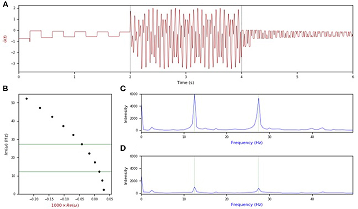
Figure 8. Response to dual-frequency stimulation. (A) Activity in the mean-field with forcing applied at time t = 2 s for a duration of 2 s and turned off afterwards. (B) Eigenvalues of the characteristic equation with positive imaginary part. The green lines indicate the resonances used to stimulate the system. The frequencies shown are ω₂ = 12.4 Hz, ω₅ = 27.4 Hz. (C) Power spectral activity from the forcing region t = 2–4 s, scaled to give the relative intensity at each frequency. The peaks of the system's response lies near two chosen forcing frequencies. (D) Power spectral activity for the post-stimulation period i.e., t = 4–6 s. The power still peaks near the two input resonances, but with far less intensity. Here τ = 200 ms, g = −1.5, D = 0.20, S₁ = S₂ = 1.

Network Simulations With Realistic Whole-Brain Anatomical Connectivity and Heterogeneous Delays

The analytic and numerical examinations of the phenomenon considered thus far have been done using simplified mean-field approximations and subsequent linear analysis (Figures 3–7) and numerical simulations of networks with topologies equivalent to uniform connectivity (Figure 2). To emphasize the relevance of these observations to real nervous systems with large, complex wiring topologies, we now study the network model described in Equation (1) using human whole-brain connectivity data. For this we used the default connectivity matrix freely available in the open-source modeling and neuroinformatics platform The Virtual Brain (TVB; https://github.com/the-virtual-brain) [28, 29]. This matrix specifies connection weights between 74 cortical and subcortical regions, with weights and directionality defined by chemical tracing data from the CoCoMac database, modified to corresponding regions in the human brain (Figures 9A,B). Additionally, we used this model to study the effects of non-uniform (distributed) conduction delays. Delay values were sampled from a Gaussian distribution with a fixed mean of 100 ms and standard deviations ranging from 1 to 10. We chose those values to see how the heterogeneous delay case departs from the unique delay case previously studied. The sampled delays were then assigned randomly to edges in the connectivity graph shown in Figures 9A,B.

FIGURE 9

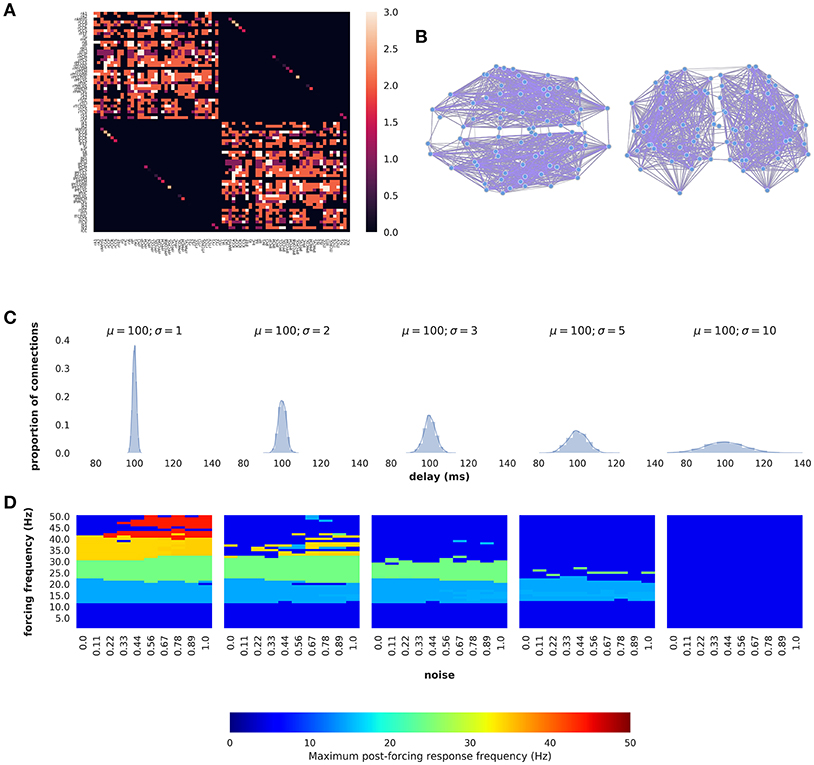
Figure 9. Persistent entrainment in a network model of large-scale human brain dynamics with realistic wiring topology and distributed delays. (A) Connectivity matrix. Row and column tick marks indicate brain region label for each node. Upper left and lower right quadrants indicate intra-hemispheric right and left hemisphere connections, respectively; upper right and lower left blocks show cross-hemispheric connections, which are restricted to corresponding regions in left and right hemispheres. (B) Physical network layout from axial (left), and coronal (right). (C) Conduction delay distributions used for the network models. (D) Entrainment vs. forcing frequency for each conduction delay distribution.

Dominant frequency responses of this system as a function of noise and forcing frequency are shown in Figure 9D for five different values of the delay distribution standard deviation σ. For low values of σ (i.e., near-uniform delays), the network model (Figure 7D, left) shows exactly the same behavior as seen in the mean-field model, with a discrete set of preferred frequencies emerging in the post-stimulation period (i.e., Figure 6B). The values of the preferred frequencies are independent of noise level, and thus appear as continuous plateaus or bands, with the dominant frequency response being the closest out of the allowed set to the forcing frequency. As σ is increases, the range of available frequency responses progressively decreases, until at σ = 10 the dominant post-forcing frequency is the same as the natural frequency (~4 Hz) for all forcing frequencies studied.

Discussion

The optimization of stimulation, in particular the control and stabilization of its aftereffects, are important aspects of both fundamental and clinical research on normal and abnormal brain dynamics. Recent studies have shown that after rhythmic entrainment, neural oscillations may remain locked to the stimulation frequency even after stimulation offset [8, 30]. This form of persistent entrainment has been linked the interaction of periodic signals with recurrent neuronal loops as well as to the presence of time delay [8], but the precise mechanism remains poorly understood. To better understand how periodic forcing may evoke this type of oscillatory response, we analyzed a generic non-linear neural network model with time delay; the model also includes noise to improve its biophysical plausibility since rhythms have different levels of coherence. Using mean-field and linear stability analyses, our results show that periodic forcing can be tuned to selectively excite intrinsic resonances of the system. In turn, this triggers persistent responses whose relaxation time exceeds the duration of time delay. We found that the delay in our model endows the system with an infinite reservoir of frequencies with different stability properties. This per se is not surprising since delays make the dynamics infinite-dimensional. However, we have shown that periodic forcing interacts with the unstable eigenmodes of our system, leading to bufferings of various durations.

Our analysis further indicates that noise acts as a resonance regulator, which can tune the response of the system by displacing the eigenvalue spectrum in the imaginary plane and thus through an effective change in linear stability. Through this change in stability, different resonances can be amplified and the buffering time can be increased. From a neuroscience perspective, this is consistent with results reporting the dependence of rhythmic stimulation effects on brain states. Assuming that different brain states may be associated with different noise levels, this noise shapes the susceptibility of neural populations to entrainment, and consequently the persistence of oscillations beyond the end of stimulation.

The results above are contingent upon linear approximations, while the original system (i.e., Equation 1) is not. In particular, for values of D where the system remains below the Hopf bifurcation threshold (i.e., stable oscillations for smaller D in Figure 3) solutions of the non-linear Equation (1) do not diverge, while solutions of the linear Equation (6) do. This discrepancy between linear and non-linear responses can be further seen in Figure 6A where the power found at the forcing frequency after offset is monotonically decreasing with increasing frequency; this contrasts with the results of Figure 4 where resonance curves show divergences at increasing intensities of noise. We add that in the low noise limit (D → 0), the response function converges to a Heaviside function, and the system is amenable to a metastability analysis in which the waveform and duration of any transient oscillations can be calculated [31].

Our analysis further demonstrates that persistent entrainment is prevalent in systems with longer time delays. Indeed, the density of resonant frequencies (number of resonances per frequency unit) increases with τ; persistent frequencies represent an increasingly larger portion of parameter space. This can be seen in Figure 4, where the number of resonant peak—and thus eigenfrequencies—increases with the delay. This implies that as τ becomes very large, the high density of resonant frequencies will converge toward a one-to-one relationship between forcing frequency and persistent frequency, allowing the system to implement an effective buffer of forcing signals through a very dense set of frequencies. This is because increasing the time delay shifts the position of the HB, allowing an increasingly large number of eigenvalues to pass toward the right-hand side of the imaginary axis. It remains to be seen if this phenomenon can be observed in noisy networks of spiking neurons and in presence of shorter time delays.

It is clear that a range of delays, arising from the variety of feedback loops that may exist in brain networks, can support reverberations across a range of periods for a certain time. In particular, when delays are sufficiently large compared to intrinsic neural response times (typically when the ratio of these time scales exceeds 1—see [27], multistability can arise in the sense that different initial conditions can lead to different steady state solutions [32]. This is apparent in the presence of a mild amount of noise or even in the absence of input [33]. From those results, it is expected that forcing a network such as the one considered here could further be sustained by multistability, beyond the basic effect described in our paper. The direct link between multistability and persistence is an interesting topic for future investigation.

Our work relates to other recent efforts to examine the buffering ability of neural networks, i.e., their capacity to temporarily store a signal over a short time delay and then play it back through readout neurons [34]. These authors considered the ability of a randomly connected spiking network (as opposed to a globally coupled network studied here) to buffer a random input signal with a short (10 ms) correlation time. Their buffering context differs a bit from that used here. Instead of focusing on network output that outlasts a stimulation, their goal is to store and shift an input signal to the neural net such that the output of the neural net is a faithful but delayed version of the input. Integrated circuits known as bucket brigade devices produce this effect, and have been used in the context of delayed dynamics to investigate e.g., multistability and the effects of noise [35]. In contrast to our network, the internal delays of the recurrent circuitry used in Major and Gerstner [34] is quite short, namely 1 ms. Their network also had a background Poisson spike train noise, and thus was noisy like ours. Buffering was measured by the reconstruction error between an injected random signal with a correlation time of 10 ms and the delayed output of the network. The error increased with increased buffering delay (i.e., with the desired delay between output and input), and buffering was deemed to be quite limited for buffering times beyond the maximal value of 20 ms investigated. Their limiting buffering time was imposed by the time scale of the network response time (20 ms). It would be interesting to explore how our network, with its significantly longer delays, could produce a buffering of such random input. The precise connection between the goals of time-shifting and controlling how activity outlasts stimulation can be sought.

Another more recent line of research at the intersection of delayed dynamics and neural computation involves reservoir computing designs that rely on a simple delay with a nonlinear element [36]. Like here, this setup endows the network with a large range of internal time scales of response, and can be used for input classification with a neuro-inspired architecture [37]. By a suitable assignment of segments of input signals to nodes in a delayed loop, in conjunction with an output weight learning rule, the network embeds the input into a larger dimensional space where hyperplanes for separating clusters (and hence for classifying) are more readily obtained. This reservoir computing, like similar non-delayed versions, relies on transient dynamics. While no explicit effort has been made to investigate the reverberation properties of these nets (with and without delays) after the input stops, we expect that they too would be able to provide buffering and memory effects that outlast the input based on the mechanisms discussed here.

It is clear that our ability to control networks to respond to certain signals and not others, and to use such effects as biomarkers for e.g., mental disease (see e.g., [38] in the context of schizophrenia), is a wide-open field in which there is much work left to do in terms of understanding the targeting and maintenance of brain states. Our work extends these dynamical ideas from the realm of manipulating brain states through stimulation to long-term targeting and control of post-stimulation states.

Author Contributions

JL, JG, and SP performed the research and analysis. JL, JG, SP, and AL wrote the paper.

Funding

We would like to thank the Natural Sciences and Engineering Research Council of Canada for funding.

Conflict of Interest Statement

The authors declare that the research was conducted in the absence of any commercial or financial relationships that could be construed as a potential conflict of interest.

References

1. Pascual-Leone A, Rubio B, Pallardó F, Catalá MD. Rapid-rate transcranial magnetic stimulation of left dorsolateral prefrontal cortex in drug-resistant depression. Lancet (1996) 348:233–7. doi: 10.1016/S0140-6736(96)01219-6

PubMed Abstract | CrossRef Full Text | Google Scholar

2. Miniussi C, Harris JA, Ruzzoli M. Modelling non-invasive brain stimulation in cognitive neuroscience. Neurosci Biobehav Rev. (2013) 37:1702–12. doi: 10.1016/j.neubiorev.2013.06.014

PubMed Abstract | CrossRef Full Text | Google Scholar

3. Romei V, Thut G, Silvanto J. Information-based approaches of noninvasive transcranial brain stimulation. Trends Neurosci. (2016) 39:782–95. doi: 10.1016/j.tins.2016.09.001

PubMed Abstract | CrossRef Full Text | Google Scholar

4. Thut G, Bergmann TO, Fröhlich F, Soekadar SR, Brittain JS, Valero-Cabré A, et al. Guiding transcranial brain stimulation by EEG/MEG to interact with ongoing brain activity and associated functions: a position paper. Clin Neurophysiol. (2017) 128:843–57. doi: 10.1016/j.clinph.2017.01.003

PubMed Abstract | CrossRef Full Text | Google Scholar

5. Kasten FH, Dowsett J, Herrmann CS. Sustained aftereffect of α-tACS lasts Up to 70 min after stimulation. Front Hum Neurosci. (2016) 10:245. doi: 10.3389/fnhum.2016.00245

PubMed Abstract | CrossRef Full Text | Google Scholar

6. Helfrich RF, Schneider TR, Rach S, Trautmann-Lengsfeld SA, Engel AK, Herrmann CS. Entrainment of brain oscillations by transcranial alternating current stimulation. Curr Biol. (2014) 24:333–9. doi: 10.1016/j.cub.2013.12.041

PubMed Abstract | CrossRef Full Text | Google Scholar

7. Neuling T, Rach S. Herrmann CS. Orchestrating neuronal networks: sustained after-effects of transcranial alternating current stimulation depend upon brain states. Front Hum Neurosci. (2013) 7:161. doi: 10.3389/fnhum.2013.00161

CrossRef Full Text | Google Scholar

8. Alagapan S, Schmidt SL, Lefebvre J, Shin HW, Frohlich F. Modulation of cortical oscillations by low-frequency direct cortical stimulation is state-dependent. PLoS Biol. (2016) 14:e1002424. doi: 10.1371/journal.pbio.1002424

PubMed Abstract | CrossRef Full Text | Google Scholar

9. Bermudez Contreras EJ, Schjetnan AG, Muhammad A, Bartho P, McNaughton BL, Kolb B, et al. Formation and reverberation of sequential neural activity patterns evoked by sensory stimulation are enhanced during cortical desynchronization. Neuron (2013) 79:555–66. doi: 10.1016/j.neuron.2013.06.013

CrossRef Full Text | Google Scholar

10. Chaudhuri R, Knoblauch K, Gariel MA, Kennedy H, Wang XJ. A large-scale circuit mechanism for hierarchical dynamical processing in the primate cortex. Neuron (2015) 88:419–31. doi: 10.1016/j.neuron.2015.09.008

PubMed Abstract | CrossRef Full Text | Google Scholar

11. Zaehle T, Rach S, Herrmann CS. Transcranial alternating current stimulation enhances individual alpha activity in human, EEG. PLOS ONE (2010) 5:e13766. doi: 10.1371/journal.pone.0013766

PubMed Abstract | CrossRef Full Text | Google Scholar

12. Lang R, Kobayashi K. External optical feedback effects on semiconductor injection laser properties. IEEE J Quant Electron. (1980) 16:347. doi: 10.1109/JQE.1980.1070479

CrossRef Full Text | Google Scholar

13. Erneux T, Larger L, Lee MW, Goedgebuer JP. Ikeda Hopf bifurcation revisited. Phys D (2004) 194:49–64. doi: 10.1016/j.physd.2004.01.038

CrossRef Full Text | Google Scholar

14. Bratsun D, Volfson D, Tsimring LS, Hasty J. Delay-induced stochastic oscillations in gene regulation. Proc Natl Acad Sci USA. (2005) 102:14593. doi: 10.1073/pnas.0503858102

PubMed Abstract | CrossRef Full Text | Google Scholar

15. Eurich CW, Milton JG. Noise-induced transitions in human postural sway. Phys Rev E (1996) 54:6681. doi: 10.1103/PhysRevE.54.6681

PubMed Abstract | CrossRef Full Text | Google Scholar

16. Solli D, Chiao RY, Hickmann JM. Superluminal effects and negative group delays in electronics, and their applications. Phys Rev E (2002) 66:056601. doi: 10.1103/PhysRevE.66.056601

PubMed Abstract | CrossRef Full Text | Google Scholar

17. Kold-Andersen L, Mackey MC. Resonance in periodic chemotherapy: a case study of acute myelogenous leukemia. J Theor Biol. (2001) 209:113–30. doi: 10.1006/jtbi.2000.2255

CrossRef Full Text | Google Scholar

18. Pfurtscheller G, Stancak A Jr, Neuper C. Event-related synchronization (ERS). in the alpha band—an electrophysiological correlate of cortical idling: a review. Int J Psychophysiol. (1996) 24:39–46. doi: 10.1016/S0167-8760(96)00066-9

PubMed Abstract | CrossRef Full Text | Google Scholar

19. Lefebvre J, Hutt A, Knebel JF, Whittingstall K, Murray MM. Stimulus statistics shape oscillations in nonlinear recurrent neural networks. J Neurosci. (2015) 35:2895–903. doi: 10.1523/JNEUROSCI.3609-14.2015

PubMed Abstract | CrossRef Full Text | Google Scholar

20. Hutt A, Mierau A, Lefebvre J. Dynamic control of synchronous activity in networks of spiking neurons. PLoS ONE (2016) 11:e0161488. doi: 10.1371/journal.pone.0161488

PubMed Abstract | CrossRef Full Text | Google Scholar

21. Asl FM, Ulsoy AG. Analysis of a system of linear delay differential equations. J Dyn Sys Meas Control (2003) 125:215–23. doi: 10.1115/1.1568121

CrossRef Full Text | Google Scholar

22. Hale JK, Lunel SMV. Introduction to Functional Differential Equations. Berlin: Springer (1993).

Google Scholar

23. Yi S, Nelson PW, Ulsoy AG. Delay differential equations via the matrix Lambert W function and bifurcation analysis: application to machine tool chatter. Math Biosci Eng. (2007) 4:355–68. doi: 10.3934/mbe.2007.4.355

PubMed Abstract | CrossRef Full Text | Google Scholar

24. Hutt A, Lefebvre J, Longtin A. Delay stabilizes stochastic systems near a non-oscillatory instability. Europhys Lett. (2012) 98:20004. doi: 10.1209/0295-5075/98/20004

CrossRef Full Text | Google Scholar

25. Lefebvre J, Hutt A. Additive noise quenches delay-induced oscillations. Europhys. Lett. (2013) 102:60003. doi: 10.1209/0295-5075/102/60003

CrossRef Full Text | Google Scholar

26. Lichtner M, Wolfrum M, Yanchuk S. The spectrum of delay differential equations with large delay. SIAM J Math Anal. (2011) 43:788–802. doi: 10.1137/090766796

CrossRef Full Text | Google Scholar

27. Mensour B, Longtin A. Power spectra and dynamical invariants for delay-differential and difference equations. Phys D (1998) 113:1–25. doi: 10.1016/S0167-2789(97)00185-1

CrossRef Full Text | Google Scholar

28. Ritter P, Schirner M, McIntosh AR, Jirsa VK. Virtual brain integrates computational modeling and multimodal neuroimaging. Brain Connect. (2013) 3:121–45. doi: 10.1089/brain.2012.0120

PubMed Abstract | CrossRef Full Text | Google Scholar

29. Sanz Leon P, Knock SA, Woodman MM, Domide L, Mersmann J, McIntosh AR, et al. The virtual brain: a simulator of primate brain network dynamics. Front Neuroinform. (2013) 7:10. doi: 10.3389/fninf.2013.00010

CrossRef Full Text | Google Scholar

30. Ronconi L, Melcher D. The role of oscillatory phase in determining the temporal organization of perception: evidence from sensory entrainment. J Neurosci. (2017) 37:10636–44. doi: 10.1523/JNEUROSCI.1704-17.2017

PubMed Abstract | CrossRef Full Text | Google Scholar

31. Grotta-Ragazzo C, Pakdaman K, Malta CP. Metastability for delayed differential equations. Phys Rev E (1999) 60:6230. doi: 10.1103/PhysRevE.60.6230

PubMed Abstract | CrossRef Full Text | Google Scholar

32. Foss J, Longtin A, Mensour B, Milton JG. Multistability and delayed recurrent loops. Phys Rev Lett. (1996) 76:708. doi: 10.1103/PhysRevLett.76.708

PubMed Abstract | CrossRef Full Text | Google Scholar

33. Foss J, Moss F, Milton JG. Noise, multistability and delayed recurrent loops. Phys Rev E (1997) 55:4536–43. doi: 10.1103/PhysRevE.55.4536

CrossRef Full Text | Google Scholar

34. Mayor J, Gerstner W. Signal buffering in random networks of spiking neurons: microscopic versus macroscopic phenomena. Phys Rev E (2005) 72:051906. doi: 10.1103/PhysRevE.72.051906

PubMed Abstract | CrossRef Full Text | Google Scholar

35. Losson J, Mackey M, Longtin A. Solution multistability in first order nonlinear differential delay equations. CHAOS (1993) 3:167–76. doi: 10.1063/1.165982

CrossRef Full Text | Google Scholar

36. Appeltant L, Soriano MC, Van der Sande G, Danckaert J, Massar S, Dambre J, et al. Information processing using a single dynamical node as complex system. Nat Commun. (2011) 2:468. doi: 10.1038/ncomms1476

PubMed Abstract | CrossRef Full Text | Google Scholar

37. Soriano MC, Brunner D, Escalona-Morán M, Mirasso CR, Fischer I. Minimal approach to neuro-inspired information processing. Front Comput Neurosci. (2015) 9:68. doi: 10.3389/fncom.2015.00068

PubMed Abstract | CrossRef Full Text | Google Scholar

38. Vierling-Claassen D, Siekmeier P, Stufflebeam S, Kopell N. Modeling GABA alterations in schizophrenia: a link between impaired inhibition and altered gamma and beta range auditory entrainment. J Neurophysiol. (2008) 99:2656–71. doi: 10.1152/jn.00870.2007

PubMed Abstract | CrossRef Full Text | Google Scholar