Two Periodic Models for the Earth-Moon System

1. Introduction

During the last years, the scientific community has increased its interest in the natural motions occurring in the Earth-Moon system. The list of possible applications is vast, for instance: the study of the far side of Moon and the relation with the translunar point L₂; the aim to exploit the cis-lunar space and the convenience of using the invariant structures related to L₁.

We have mentioned a couple which are specifically related to the Lagrangian points but, obviously, the list goes on covering a wide range of interests. Efficient mission designs depend ultimately on the understanding of the natural dynamics. To fulfill this goal, it is advisable to use simplified models. Simple models allow us to understand the underlying mechanisms that lead to interesting phenomena. From the dynamical systems point of view, the comprehension of the invariant structures (and their stability) of simple models has helped to shed light on difficult problems such as the motion of asteroids through the solar system, station keeping of spacecraft and taking advantage on the natural dynamics to design spacecraft missions. Perhaps the most illustrative example for the purpose of this work is the existence of the Trojan asteroids that can be predicted using the effective stability of the triangular points of the Sun-Jupiter Restricted Three Body Problem (RTBP). This example is convenient for the purposes of this work because the existence of objects in the triangular points has a counterpart in the Earth-Moon system: the Kordylewsky clouds. We shall come back to this example during this work (section 4.3)but, for the moment being, we want to stress that the existence of these clouds cannot be established by using the same theoretical mechanisms as the Trojan asteroids [1–3]. In fact, the literature related to the Kordylewsky clouds has been stumbling around the existence or nonexistence of objects in the Earth-Moon triangular points, mostly because of the lack of observations. Therefore, it is convenient to analyze whether a simple model is suitable for the problem we want to study.

The Earth-Moon RTBP is the most used simple model for the motion of a small body in the Earth-Moon system. There is, however, a remarkable number of works that take into account the presence of Sun's gravitation (see, for instance, [4–8]). Indeed, the most relevant effect ignored by the Earth-Moon RTBP is the gravitational attraction of Sun. In this respect, a simple model to study the dynamics near the Earth-Moon system needs to take into account Solar gravity. The problem has a natural non-autonomous periodic time dependence formulation. An advantage of the periodic models is that they can be handled by means of a stroboscopic map i.e., the map defined by the evaluation of the flow at the period of the vectorfield. This is crucial because, while the complexity of the system increases, the study of maps (even if they are numerically defined) is, in some aspects, more comfortable than the study of flow. In periodic time dependent systems, the simplest invariant objects, the ones the dynamics is organized from, are the periodic orbits with the same period as the vectorfield. These periodic orbits appear as fixed points of the stroboscopic maps and their robustness is assured by the classical Implicit Function Theorem. We would like to remark that, in quasi-periodic models the simplest invariant objects are invariant tori. The computation and study of these objects is more difficult. The discussion in this paragraph vindicates a closer look to periodic models for the Earth-Moon system. We have selected two among the literature, the Bicircular Problem (BCP) and the Quasi-Bicircular Problem (QBCP). Both models include Sun's gravity and can be written as periodic perturbations of the RTBP.

The BCP is a restricted four body problem [9, 10]. There are three primaries and a fourth, massless, test particle. In our case, the three primaries are Earth, Moon and Sun. However, this model has been utilized in other cases [11]. It is assumed that Earth and Moon move as in the RTBP, that is, along a circular orbit around its common center of masses. Let us name C_EM this barycenter. Name C_SEM the center of masses of the Sun-C_EM system. As Moon and Earth move, it is assumed that Sun and C_EM move in another circular orbit around C_SEM. We refer to Gómez, et al. [12] for a detailed derivation of the equations of motion. The BCP is a periodic perturbation of the RTBP that takes into account the direct gravitational effect of a third primary (in our case, Sun) on the particle. This model captures the non-stable character of the triangular points. Henceforth, it is suitable to use it when studying problems related with these locations (see, for instance, [13, 14]). A remarkable shortcoming of the BCP is its lack of coherence i.e., the motion assumed for the primaries does not verify Newton's laws. Moreover, the BCP has no translunar dynamical structure. This justifies the seek for a more complex model for the study of, at least, the L₂ point.

The QBCP is a version of the four body problem. It is conceived to be a coherent counterpart of the BCP. This model was introduced by C. Simó, and it has been used in several works, see [15–17] and, more recently, [18]. A characteristic of the BCP is the lack of coherence of the bicircular solution assumed for the primaries. However, there exist solutions of the three body problem which are close to bicircular [19]. To build the QBCP it is necessary to compute a quasi-bicircular solution of the three body problem, in this case, for the Earth-Moon-Sun case. There are several ways to do such a thing. In Andreu [15], Andreu and Simó [16], and Andreu [17] the authors build a specific algebraic manipulator and compute directly the Fourier coefficients of the quasi-bicircular solution. In Gabern [20], Gabern and Jorba [21], and Gabern et al. [22] the authors use a continuation scheme to compute the desired solution starting from a solution of the two body problem. After that, a Fourier transform is applied to get the Fourier coefficients of the solution. The QBCP is suitable for the study of the collinear points, especially L₁ and L₂.

With this paper, we aim to provide a general insight about the dynamics of these models for a particle in the Earth-Moon system. We care about (practical) stable motion near the triangular points and, to do so, we use the BCP. We also study invariant manifolds related to the collinear points in the QBCP. We believe that the value of this work is, precisely, giving a wide perspective and help the interested reader to choose a suitable simple model to face a first exploration related to a problem concerning the Earth-Moon system.

The paper is organized as follows: section 2 is devoted to a brief description of the RTBP. We explain how the phase space near the Lagrangian points is organized referencing some remarkable works and mentioning the techniques used to study the problem. In section 3 we give some words on the stroboscopic maps and periodic time-dependent Hamiltonian systems. We also explain how to compute high order unstable manifolds related to fixed points using the parameterization method with single and parallel shooting. Section 4 describes how the BCP can be used to study the motion near the triangular points. The advantage of this model with respect to the RTBP is that it captures the unstable character of the triangular points in the real system. The results presented are mainly devoted to stable motion in an extended vicinity of the triangular points. In section 5 we describe results concerning the QBCP. We focus on the unstable manifolds related to the periodic orbits that replace the collinear points. Finally, section 6 is devoted to conclusions and section 7 to technical details.

2. Restricted Three Body Problem

The (Circular) RTBP is a simplified model for the motion of a massless particle under the gravitational attraction of two massive bodies, the so-called primaries [23]. The primaries are assumed to revolve along circular orbits around their common center of masses. It is usual to take units of masses so the sum of the masses of the primaries is equal to one. The units of length are taken so the distance between the primaries is equal to one and the units of time are taken so the period of the revolution of the primaries is equal to 2π. It is also standard to take a rotating frame of reference that fixes the primaries at the horizontal axis. The RTBP is an autonomous Hamiltonian system with three degrees of freedom. The Hamiltonian function writes as:

$\begin{array}{rc}{H}_{RTBP}=\frac{1}{2}(p_x^2+p_y^2+p_z^2)-x{p}_y+y{p}_x-\frac{1-\mu }{r_{PE}}+\frac{\mu }{r_{PM}},& (1)\end{array}$

where $r_{PE}^2={(x-\mu )}^2+y^2+z^2$ and $r_{PM}^2={(x-\mu +1)}^2+y^2+z^2$. The parameter μ is called the mass parameter and it is the mass of the smallest primary. In the case of the Earth-Moon system μ ≈ 0.012. It is well known that the RTBP has five equilibrium points (see Figure 1). Three of them, the collinear points, are located in the horizontal axis. The other two, the triangular points, are located at the third vertex of an equilateral triangle whose other two vertices are the position of the primaries.

FIGURE 1

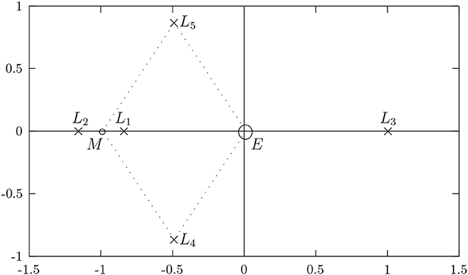
Figure 1. The restricted three body problem.

The only integral of motion of the RTBP is its Hamiltonian. In many texts, this integral of motion is presented under a slightly different form as the Jacobi integral. Each surface level of this integral is a five dimensional manifold. If the velocities are set to zero, this defines the so-called Zero Velocity Surface. These surfaces separate the configuration space in different regions. The trajectories of the system cannot cross the boundary between two of these regions. The shape of these regions change with the value of the Jacobi integral. As the Lagrangian equilibrium points are critical points of the Jacobi integral, the topology of these regions change when the energy value crosses the value associated to one of the Lagrangian points (for more details, see [23]).

The three collinear points are of type saddle×center×center. This means that, under generic conditions, a 4-dimensional center manifold emerges from each of these points. These manifolds are tangent to the elliptic eigendirections at the points. There exist, as well, one dimensional stable and unstable directions emerging tangentially to the hyperbolic eigendirections. Moreover:

• By the Lyapunov Center Theorem [24], two families of periodic orbits, the Lyapunov families, emanate from the equilibria. One of the families is born tangent to the (z, p_z) plane so it is called vertical family. The other family is contained in the (x, y, p_x, p_y) plane and it is called horizontal family. One can parametrize each family by the amplitude of the orbits. The horizontal families related to L₁ and L₃ can be continued up to trajectories which collide with Earth. The horizontal family related to L₂ can be followed up to collisions with Moon. The vertical families end up in bifurcating planar orbits [12, 25].

• The Lyapunov families can be regarded as the non-linear continuation of the harmonic oscillator given by each elliptic direction of the linearization around the equilibria. When the amplitude tends to zero, the frequency of the family tends to the normal modes of the equilibria.

• As the frequency varies, the horizontal family undergo a 1:1 resonance and the Halo [12, 26–28] family are originated (by means of a pitchfork bifurcation). Secondary families of Halo-type orbits appear by duplication and triplication of the main family [29, 30].

The center manifold can be computed by means of normal form techniques [31–33], with the parametrization method [34–37] and also numerically [29]. The dynamics restricted to the center manifold can be described by a Hamiltonian with two degrees of freedom. By fixing a level of energy and taking a Poincaré section, one can reduce the problem to the study of a family of area preserving maps. This methodology suffices to observe the phase space during the bifurcation that give rise to the Halo families.

2.1. Motion Near the Triangular Points

The Earth-Moon triangular points of the RTBP are linearly stable [23]. KAM theory can be used to establish the existence of a dense set of Lagrangian invariant tori close enough to the equilibria [38]. This has important consequences on the nonlinear stability of the triangular points. If we restrict ourselves to the planar case, these KAM tori (of dimension two) act as barriers for the dynamics in a fixed level of energy. Therefore, KAM tori enclose stable motion for initial conditions which are close enough to the triangular points. This argument based on KAM theory falls apart in the spatial case. Indeed, Lagrangian tori have, in that case, dimension three and the phase space, for a fixed level of energy, is five dimensional. There is, in general, no way to avoid Arnold diffusion [39]. However, using normal form techniques, it is possible to derive bounds on the diffusion time [40] (these techniques can be extended to the periodic [41] and the quasi-periodic case [42]). These, make us think about regions of practical stability i.e., regions in which the motion is non-stable but initial conditions take a long time, maybe longer than the expected age of the solar system, to escape. These theoretical results are valid for a small region near the triangular points and numerical simulations provide evidences of large regions of practical stability [43].

It is natural to look for other invariant structures that play a remarkable role to define the shape of the (numerically computed) region. In this regard, [43] provides numerical evidence on the role of the center-unstable and center-stable manifolds of the collinear point L₃. These manifolds are of dimension five and act as barriers of the dynamics. Obviously, the motion driven by these manifolds escape from the vicinity of the triangular points at some moment, but, again, the required time to do so can be large.

3. Periodic Time-Dependent Hamiltonians and Stroboscopic Maps

The alternatives to the RTBP presented in this paper, the BCP and the QBCP are both periodic time dependent Hamiltonian systems that can be seen as perturbations of the RTBP. Because of this periodic time-dependence, the Lagrangian points are no longer equilibria but they are replaced by minimal periodic orbits i.e., periodic orbits with the same period as the perturbation. These periodic orbits are known as the dynamical equivalents of the Lagrangian points. The usual tools to study numerically the RTBP are the combination of fixing suitable energy levels and suitable Poincaré sections. We note that, in time dependent models like the BCP and the QBCP the Hamiltonian is no longer preserved. A standard tool to deal with these periodic time-dependent systems is the so called stroboscopic map: Let ${U}\subset {ℝ}^n$ be an open set, T the period of the vectorfield and $\phi :\left[0,T\right]\times ℝ\times {U}\mapsto {ℝ}^n$, where φ(t₀, t, x₀) stands for the solution which, at time t₀ lies at x₀ evaluated at time t, the flow of the differential equation. We define the stroboscopic map for $x\in {U}$ as f(x) = φ(0, T, x). In this work we care about Hamiltonian differential equations. In this case, the stroboscopic map is symplectic.

3.1. Invariant Structures

The simplest invariant objects of the original system are periodic orbits with the same period as the vectorfield. These appear as fixed point of the stroboscopic map. The monodromy matrix associated to these periodic orbits is the differential of the stroboscopic map. The eigenvalues of this matrix determine the linear behavior around the fixed points and, under generic conditions, give some insight about the local non-lineal dynamics. In the symplectic case, under generic conditions, each elliptic direction give rise to a family of invariant curves which can be parametrized by the frequency ([44]). This frequency approaches to the normal mode responsible form the birth of the family at the fixed point. Along the hyperbolic directions, unstable (stable) manifolds depart (arrive) from the fixed points. These invariant objects are crucial to understand the dynamics of the system.

In this paper we focus on the information that can be extracted from the computation of invariant curves and high order approximations of unstable invariant manifolds. While it is quite common, in the literature related astrodynamics, to find discussions on the computation of invariant tori of maps [13, 45, 46] it is not so usual for high order approximations of stable/unstable manifolds.

3.2. High Order Approximation of Unstable Manifolds Using the Parametrization Method

Let ${U}\subset {ℝ}^n$ be an open set and assume that we are given a map $f:{U}\mapsto {ℝ}^n$ induced by the evaluation at time T of a flow of some ordinary differential equation (stroboscopic map). The following discussion can be done for any Poincaré map as well. Here we assume that the section is temporal for simplicity of the exposition and because it is the natural section to chose in a periodically perturbed autonomous system. Let us suppose also that $\bar{x}\in {U}$ is a fixed point i.e., $f(\bar{x})=\bar{x}$. Obviously $\bar{x}$ is an initial condition for a T-periodic orbit of the original flow. The linearized normal behavior around the fixed point is given by the eigenvalues of the differential of the map evaluated at the point. Assume specDf = {λ, λ₂, …, λ_n} with |λ| > 1. Under generic conditions, we know that there exist a 1-dimensional unstable invariant manifold related to the fixed point. That is, there exist an open interval I ⊂ ℝ and a map $x:I\mapsto {U}$ such that $x(0)=\bar{x}$ and

$\begin{array}{rc}f(x(s))=x(\lambda s).& (2)\end{array}$

Equation (2) is known as the invariance equation of the invariant manifold. The parametrization method [47–50] is a powerful tool to, both, prove the existence of the manifold and compute it. The idea is to expand the parameterization of the manifold in Taylor series at s = 0 and solve Equation (2) order by order. This makes sense in the case when both the map and the manifold are analytic. This assumption is fulfilled by the applications we are interested in. Hence, the goal is to compute a semi-analytic approximation of a parametrization of the invariant manifold. Let us name

$x(s)={\displaystyle \sum _{j=0}^{\infty }}{a}_j{s}^j.$

We are interested in numerically compute the coefficients a_j for j = 0, …, d for a given degree d. This is achieved by a recurrent scheme in which we solve Equation (2) order by order:

• Order 0 is given by the coordinates of the fixed point.

• Order 1 is given by the eigenvector related to λ.

• For k > 0, order k + 1 is given by the solution of the following linear system:

$(Df(0)-{\lambda }^{k+1}I)a_{k+1}=-b_{k+1}.$

Here, b_k+1 is the k+1-th term of the evaluation of the manifold up to degree k by the map f, that is:

$f_{\le k+1}(x_{\le k}(s))={\displaystyle \sum _{j=0}^k}{b}_j{s}^j+b_{k+1}{s}^{k+1},$

where the subindices (·)_{≤ k+1} denote the truncation of the power expansion of (·) at order k + 1.

Notice that it is mandatory to have a method to compose power expansions of the manifold with the map itself. Sometimes, when, the map is explicit, one is able to find a suitable recurrence expression to compute the terms of this composition. If a recurrence is not available one can compute higher order terms by automatic differentiation¹. In the case we are interested, the map is not given explicitly but comes from a numerical integration of a differential equation. Here, the only reasonable strategy seems to use Jet Transport. This technique is based in the idea of, instead of integrating a single point, integrate a function given by its expansion in Taylor series. That is, one transports the jet, the set of derivatives of the function at a given point, up to a given order. It is straightforward to construct an integrator of jets from an integrator of numbers. It is only a matter of replacing the standard floating arithmetic by a polynomial arithmetic [Farrés et al., to appear].

There is another obstacle that can appear when dealing with Poincaré maps: if the orbit is very unstable, the hyperbolic direction may lead to a huge error propagation. This problem can be avoided by using parallel shooting. The idea behind parallel shooting is to enlarge the dimension of the system in order to decrease the time of integration. Let us denote by ${\phi }_{t_0}^{t_f}(x)$ the solution of the differential equation with initial condition (t₀, x) evaluated at time t_f. Fix k ∈ ℕ, the number of sections, and set h = T/k. For i = 0, …k, we define τ_i = ih. If m = nk, we define the function $F:{V}\mapsto {ℝ}^m$

$F:\left(\begin{array}{c}{x}_1\\ x_2\\ ⋮\\ x_k\end{array}\right)\mapsto \left(\begin{array}{c}{f}_k(x_k)\\ f_1(x_1)\\ ⋮\\ f_{k-1}(x_{k-1})\end{array}\right).$

Here ${V}={{U}}^k$ is an open set of ℝ^m, and, for $x\in {U}$, $f_j(x)={\phi }_{{\tau }_{j-1}}^{{\tau }_j}(x)$. The differential map DF is given by

$DF=\left(\begin{array}{cccc}0& \dots & \dots & D{f}_k\\ D{f}_1& \dots & \dots & ⋮\\ ⋮& \dots & \dots & ⋮\\ 0& \dots & D{f}_{k-1}& 0\\ \end{array}\right).$

For $\bar{x}\in {U}$, name y = (x₁, …, x_k) where $x_1=\bar{x}$ and x_j = f_j(x_j−1) if 1 < j ≤ k. Then:

1. y is a fixed point of F if and only if $\bar{x}$ is a fixed point of f.

2. The duple (ζ, v = (v₁, …, v_k)), ζ ∈ ℂ and $v_k\in {ℂ}^n$ is a pair eigenvalue/eigenvector of DF(y) if and only if $({\zeta }^k,v_1)$ is a pair eigenvalue/eigenvector of $Df(\bar{x})$.

3. The projection to the first coordinate of the invariant manifold of F related to ζ coincides with the invariant manifold of f related to ζ^k = λ.

4. The Bicircular Problem and the Triangular Points

The BCP is a perturbation of the RTBP. It is usual to take the units and the synodic coordinates of the Earth-Moon RTBP (see Figure 2). The BCP is not coherent, that is, the trajectories followed by the primaries do not obey Newton's laws. This is not an inconvenient since the model has been shown to be useful to describe the dynamics near the triangular points [51]. As a dynamical system, the BCP is a Hamiltonian system with three and a half degrees of freedom, i.e., a non-autonomous periodically time dependent with three degrees of freedom. The Hamiltonian function, written in the RTBP coordinates and units, is given by

$\begin{array}{l}H=\frac{1}{2}(p_x^2+p_y^2+p_z^2)-x{p}_y+y{p}_x-\frac{1-\mu }{r_{PE}}-\frac{\mu }{r_{PM}}\\ -\frac{m_S}{a_S^2}(ysin\theta -xcos\theta )-\frac{m_S}{r_{PS}}.& (3)\end{array}$

FIGURE 2

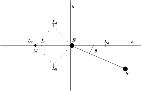
Figure 2. The bicircular model.

Here μ, r_PE and r_PM denote the same quantities as in (1). Moreover, m_S denotes the mass of Sun, a_S the averaged semi-major axis of Sun, θ = ω_St, ω_S is the frequency of Sun in this system of reference, $T_S=\frac{2\pi }{{\omega }_S}$ is its period and finally, $r_{PS}^2={(x-a_{S}cos\theta )}^2+{(y-a_{S}sin\theta )}^2+z^2$. Notice that this Hamiltonian can be splitted in two parts:

$H_{BCP}=H_{RTBP}(X)+H_S(\theta ,X).$

The time dependent part contains two terms, the Coriolis effect due to the rotating frame of coordinates and Sun's gravitational potential. The Taylor expansion of the potential starts with

$\frac{1}{a_S}\left(1+\frac{xcos\theta -ysin\theta }{a_S}\right).$

Therefore, the Hamiltonian, if we truncate the Sun's potential at linear order is written as

$H_{BCP}^{<2}=H_{RTBP}-\frac{m_S}{a_S}.$

So, the Coriolis term and the truncated Sun's potential cancel out and the dynamics is the one of the RTBP. This is to say that the contribution due to Sun's potential starts at order two, that is, the BCP is a periodic time dependent perturbation with size ${O}(\frac{m_S}{a_S^3})\approx 0.0056$. Anyhow, it is large enough to produce remarkable changes on the dynamics, especially near the triangular points. In Figures 3 (left), 6 (left) we display continuations from the RTBP to the BCP. The vertical axis in these plots represent an artificial parameter ε which multiplies the mass of Sun. Therefore, when ε = 0 the model corresponds to the RTBP and, when ε = 1 the model corresponds to the BCP. We shall comment these figures in detail in the next sections.

FIGURE 3

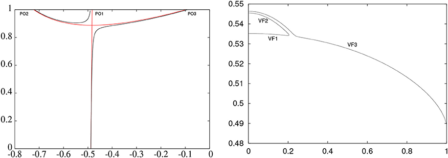
Figure 3. Left: Continuation of L₄ as a periodic orbit with respect to the mass of Sun. Horizontal axis: x. Vertical axis: ε. The black curve stands for the continuation to the BCP. The red curve for the truncated version of the BCP. See text for more details. Right: Vertical families of 2D tori for the BCP. The horizontal axis is the p_z coordinate and the vertical axis displays the frequency. See text for more details.

4.1. Dynamical Equivalents of the Triangular Points

First of all let us mention that, due to a symmetry, the dynamics near L₄ is the same as the dynamics near L₅ (in fact, this symmetry maps orbits in the region y > 0 to orbits in the region y < 0). A feature of the BCP to be stressed is that the region around the geometrically defined triangular points is unstable. The influence of Sun's potential is enough to produce a bifurcation in the periodic orbit that replaces L₄ (i.e., L₅). It is well known [51] that each triangular point is replaced by three periodic orbits with the same period as Sun. One small and unstable (the actual replacement of L₄) and two which are stable. We have named these orbits PO1, PO2, and PO3. See Figure 3 (left) a continuation diagram from the RTBP to the BCP. The two additional periodic orbits are produced by an imperfect pitchfork bifurcation (i.e., a pitchfork bifurcation broken due to a loss of symmetry).

One may ask which is the model that displays the perfect bifurcation and which is the broken symmetry. To address this question we take a look at the order two of the Taylor expansion of Sun's gravitational potential. We have

$H_S^2(\theta ,x,y,z)=\frac{1}{a_S^3}\left(\frac{3}{2}T{(x,y,\theta )}^2-\frac{1}{2}(x^2+y^2)\right).$

We have named T(x, y, θ) = −x cos θ + y sin θ. We would like to stress again that $H_S^2$ is the first contributing non-autonomous term in the model due to the cancellation produced by the Coriolis acceleration. This term is invariant under the symmetry (x, y, x, θ)↦ (x, −y, x, −θ). The order three of the expansion is given by:

$H_S^3=\frac{1}{a_S}\left({\left(\frac{\rho }{a_S}\right)}^3\frac{\frac{5}{2}{T}^3-\frac{3}{2}T}{a_S\rho }\right).$

Here ρ² = x² + y². The polynomial in T is no longer even. This breaks the symmetry and, hence, the pitchfork bifurcation. The non-autonomous model that displays the perfect bifurcation is:

$H_{BCP}^{\le 2}=H_{RTBP}(X)+H_S^2(X,\theta ).$

The perfect (non broken) pitchfork bifurcation in Figure 3 (left, curve in red) shows the continuation diagram from the RTBP to this simplified version of the BCP. Due to the symmetry, periodic orbits PO2 and PO3 only differ on the phase on the orbit.

4.2. Phase Space of the Stroboscopic Map Near the Triangular Points

The three periodic orbits appear as fixed points of the stroboscopic map. We recall that their linear normal behavior is of type saddle×center×center for PO1 and totally elliptic for PO2 and PO3. There are several ways to justify that, from the elliptic directions of each fixed point, there is a family of invariant curves whose frequency tends to the normal modes of the fixed points [44, 52].

Therefore, we have a family of invariant curves for each elliptic direction, that is, two for PO1 (HF1 in the horizonal plane and VF1 in the vertical direction), three for PO2 (HF2F1 and HF2F2 are horizontal, and VF2 is vertical) and three for PO3 (HF3F1 and HF3F2 horizontal, and VF3 vertical). The remaining eigendirection of PO1 is hyperbolic. There exist stable and unstable one-dimensional invariant manifolds associated to these hyperbolic directions. Initial conditions near the triangular points shadow the unstable manifold which wonder some time around the periodic orbits PO2 and PO3 and finally abandon the vicinity of the triangular points. These manifolds are of special interest if one plans to put or take out objects near L₄ and L₅. The stable and unstable manifolds related to PO1 can be computed up to high order directly on the stroboscopic map (section 3.2 and [Farrés et al., to appear]). In Figure 4 we observe a projection of the phase portrait of the map. The three points displayed with crosses correspond to PO1 (in the middle), PO2 and PO3. It is displayed as well, semianalytical approximations of the stable and unstable invariant manifolds. We have used an approximation of order 64. The width curve are the pieces given by the parameterization. The thin curve correspond to some iterations of these pieces. It can be observed, also, some invariant curves growing from PO2 and PO3. These invariant curves are totally elliptic near the fixed points.

FIGURE 4

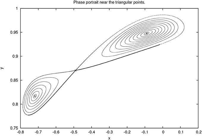
Figure 4. Stroboscopic map near the triangular points: Horizontal axis x. Vertical axis y. See text for more details.

4.3. Regions of Effective Stability Near the Triangular Points

As we have observed, the triangular points are replaced by three periodic orbits, one of them unstable. This is the reason why the BCP is an interesting model [12]. Indeed, the unstable manifold of the triangular periodic orbit takes initial conditions away from the vicinity of the triangular points. However, we can pursue on the seek for regions of (effective) stability out of the plane of motion of the primaries. The mechanism that suggest the existence of regions of effective stability is the stickiness of normally elliptic low dimensional invariant tori. See [41, 52]. As we discussed before, there are families of invariant tori emanating from the periodic orbits PO2 and PO3. These families are elliptic close enough to the fixed points. This results on two small regions of effective stability in the plane of motion of the primaries related to the totally elliptic orbits.

We put our attention on the vertical families (one for each orbit) of invariant tori. In Figure 3, Right, we display how these families vary when they grow out of the plane of motion of the primaries. We observe that the three families display a broken pitchfork symmetry, analogous to the one of the periodic orbits. The linear normal behavior of the tori is the same as the periodic orbit near the plane. As a consequence of the pitchfork bifurcation, at some some distance of the plane, the surviving family is totally elliptic. Therefore, the tori are sticky and regions of effective stability are to be expected. We label these families VF1, VF2 and VF3 after the corresponding periodic orbits. The families VF1 and VF2 are connected, as it happens with PO1 and PO2. On the other hand VF3 reaches high amplitudes in the (z, p_z) plane. It is known that, skipping resonances, the three families have the same stability as the corresponding periodic orbits. Therefore, the tori of VF1 have hyperbolic directions while the ones of VF2 are normally elliptic (except for small intervals of instability produced by resonances involving internal and normal frequencies). Recall that both families are connected and the change of stability takes place at a turning point. The tori of VF3 are normally elliptic up to very high values (again, except for resonances).

Normally elliptic lower dimensional tori induce regions of effective stability. Numerical estimations of the shape and the size of these regions show that, in the case of VF2, the regions are small and narrow while in the case of VF3 large regions exist for sufficiently high values of the vertical amplitude. In Figure 5 we show two stability regions out of the horizontal plane. These regions seem to persist in the real model for time spans of 1,000 years [14, 53]. The effect of Solar Radiation Pressure on the effective stability regions of the BCP is discussed in Jorba-Cuscó et al.[54].

FIGURE 5

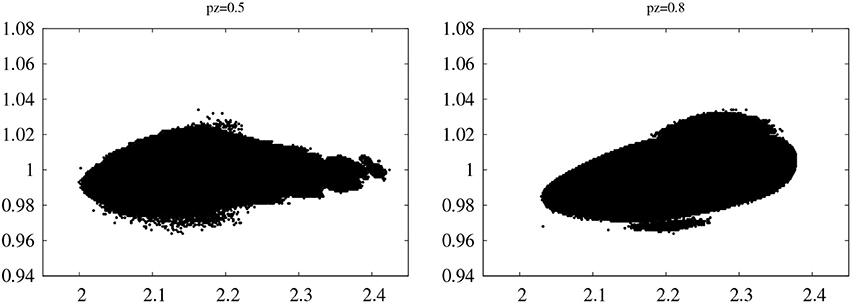
Figure 5. Stability regions with initial conditions on the tori of the VF3 identified by p_z = 0.5 and p_z = 0.8. Horizontal axis: α. Vertical axis r. See text for more details.

Let us explain how Figure 5 is obtained. Each of the vertical family of invariant tori can be identified by the value of the coordinate p_z when z = 0 and p_z > 0. Denote by $a(p_z)\in {ℝ}^6$ the coordinates of the point that identifies a torus. We have to select a set of initial conditions near a(p_z) and integrate them for a long time span. Let us be more precise on how to select the initial conditions. We use a two dimensional grid, the coordinates z, p_x, p_y and p_z will be fixed by the corresponding values of a(p_z). To adapt to the shape of the regions, we use a polar-like grid, centered at Earth:

$\{\begin{array}{c}{x}_{ij}=r_{i}cos{\alpha }_j+\mu ,r_i=1+i{h}_r,\\ y_{ij}=r_{i}sin{\alpha }_j,{\alpha }_j=2\pi j{h}_{\alpha },\end{array}$

where h_r and h_α are used to control the density of the grid. The computation goes as follows. Take a point of the grid and integrate the vector field 15000 Moon revolutions. At each integration step, we test if there is a collision with Earth or Moon. If there is a collision, or the coordinate y becomes negative, we stop the integration (Recall that we are interested in the points that remain close to L₄). We have used h_r = 0.001 and h_α = 0.0002. The difference on the sizes of these small quantities is aimed to produce a nearly squared grid.

4.4. A Weakness of the BCP

The translunar point is one of the most interesting locations at the Earth-Moon system. The reason is that L₂ seems suitable to observe the far side at Moon. Taking into account that, a natural criticism to the BCP is that it does not have a dynamical replacement of L₂. In Figure 6 (left) it is displayed a continuation of L₂ as a periodic orbit from the RTBP to the BCP. The periodic orbits are identified by their coordinates as fixed points of the Stroboscopic map. These orbits have been computed by means of the parallel shooting method. Again, the vertical axis is an additional parameter, ε, multiplying the mass of Sun. The point L₂ is the middle crossing of the characteristic curve with the homotopy level corresponding to the RTBP, at the bottom. The other two points of the RTBP correspond to the same 1:2 resonant planar Lyapunov orbit but with different initial times. We observe that the continuation of L₂ reaches a turning point and it never reaches the homotopy level of the BCP. The result is that the translunar dynamical structure is lost in the BCP. This suggest that a more complex model needs to be used to analyze the natural behavior near the translunar point. The resonant Lyapunov orbit can be continued to the BCP. The result is a large orbit that remains away from the translunar point, see Figure 6 (right).

FIGURE 6

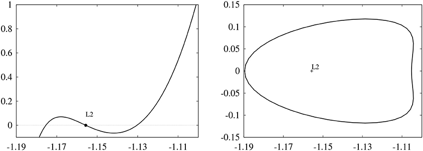
Figure 6. Left: Continuation of L₂ as a periodic orbit with respect to the mass of the Sun. Horizontal axis: x. Vertical axis: ε. See text for more details. Right: Periodic orbit near L₂ in the BCP. Horizontal axis: x. Vertical axis: y.

5. The Quasi-Bicircular Problem and the Collinear Points

The quasi-bicircular solution of the Earth-Moon-Sun system is planar i.e., the three bodies move in the same plane. After the quasi-bicircular solution is computed one can write the equations of motion of the test particle, prescribing the quasi-bicircular solution as motion for the primaries. It is usual to compute the quasi-bicircular solution in the Jacobi frame, however, if one has the purpose of describing the dynamics in the Earth- Moon vicinity, it is suitable to use the frame of coordinates corresponding to the Earth-Moon RTBP. To do so, one has to perform three different transformations. First, one has to use a translation to move the origin from the global barycenter to Earth's and Moon's center of masses. Second, one has to use a rotating (synodic) frame to keep Earth and Moon fixed on the horizontal axis. Third, the unit of length is scaled so the distance between Earth and Moon is equal to one. The units of mass and time which are usually selected in the Earth-Moon RTBP can be imposed already in the Jacobi formulation of the Three Body Problem.

The resulting model is a Hamiltonian system with three and a half degrees of freedom. The Hamiltonian function can be written as

$\begin{array}{l}H=\frac{1}{2}{\alpha }_1(p_x^2+p_y^2+p_z^2)+{\alpha }_2(p_{x}x+p_{y}y+p_{z}z)+{\alpha }_3(p_{x}y-p_{y}x)\\ +{\alpha }_{4}x+{\alpha }_{5}y-{\alpha }_6\left(\frac{1-\mu }{r_{pe}}+\frac{\mu }{r_{pm}}+\frac{m_S}{r_{ps}}\right),& (4)\end{array}$

where, $r_{pe}^2={(x-\mu )}^2+y^2+z^2$, $r_{pm}^2={(x-\mu +1)}^2+y^2+z^2$, $r_{ps}^2={(x-{\alpha }_7)}^2+{(y-{\alpha }_8)}^2+z^2$, and for i = 1, …, 8 α_i: 𝕋 ↦ ℝ are periodic functions. That is,

$\begin{array}{rc}{\alpha }_i(\theta )=a_0^i+{\displaystyle \sum _{k\ge 0}}{a}_k^{i}cosk\theta +{\displaystyle \sum _{k\ge 0}}{b}_k^{i}sink\theta .& (5)\end{array}$

Here, θ = ω_St and ω_S is the frequency of Sun. Moreover, α_i is odd for i = 1, 3, 4, 6, 7 and even for i = 2, 5, 8. Obviously one can only have a numerical approximation of these functions. In this case, we take advantage on the computations done in [15] and take the same values for the Fourier coefficients of the periodic functions α_i's. To end, and taking into account the properties of the functions α_i's, it is easy to see that the Hamiltonian function (4) has the symmetry (θ, x, y, z, ẋ, ẏ, ż)↦(−θ, x, −y, z, −ẋ, ẏ, −ż), ẋ = p_x+y, ẏ = p_y− x, ż = p_z.

The meaning of these periodic functions is the following:

1. (α₇, α₈, 0) is the position of Sun in the plane of motion of the primaries.

2. α₁, α₂, α₃ and α₆ capture the fact that the distance between Earth and Moon is not constant.

3. α₄ and α₅ take into account the Coriolis effect due to the rotating frame of reference.

5.1. Dynamical Equivalents of the Collinear Points

In this section we give some words about the minimal periodic orbits that replace the collinear points in the QBCP. In Figure 7 we display the dynamical equivalents, from left to right, of L₁, L₂ and L₃. We observe that the orbits replacing L₁ and L₂ are small, their maximal distance to the corresponding equilibrium point is of order ${O}(10^{-6})$. As the original equilibrium points, the linear normal behavior of these orbits is of type saddle×center×center. In Table 1 we display the eigenvalues of each orbit. We notice that the unstable direction of L₁ (of order 10⁸) and the unstable direction of L₂ (of order 10⁶) are large and this implies huge propagation of error near these orbits. On the other hand, the dynamical equivalent of L₃ has a very weak unstable direction, at least compared to the other two.

FIGURE 7

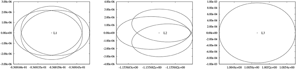
Figure 7. Dynamical equivalents of the collinear points. Left: L₁. Center: L₂. Right: L₃. Horizontal axis: x. Vertical axis: y. See text for more details.

TABLE 1

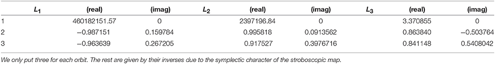
Table 1. Eigenvalues of the three dynamical equivalents of L₁, L₂ and L₃.

5.2. Resonant Orbits of Low Order

As the QBCP is a T_S-periodic system, the simplest invariant objects are T_S-periodic orbits. We already have mentioned that the equilibrium points are replaced by these periodic orbits of minimal period. Periodic orbits of the RTBP whose frequency is resonant with the one of Sun also persist as T_S-periodic orbits in the QBCP. The Lyapunov and Halo families of periodic orbits related to the equilibrium points L₁ and L₂, are a source for these kind of resonant orbits. In contrast with the families related with L₃, the families of the two first libration points are nourished with low order resonant orbits. A relation of low order resonant periodic orbits of the RTBP can be found in [15]. In [29] the authors show the ranges for the admissible periods for each family. The families related to L₃ are of relatively large period and there are not many periodic orbits whose frequency are in low order rational relation with the frequency of Sun. There is, however, a 1:1 resonant periodic orbit near the end of the vertical family. This orbit is enormous in size and cannot be considered in the vicinity of L₃. In Table 2 details of the continuations of low order resonant orbits from the RTBP to the QBCP are given: The first column corresponds to resonant periodic orbits of the RTBP. The label in this first column consist in three numbers that encode each orbit. The first is a zero and indicates that the orbit belongs to the RTBP (this is intended to distinguish them from the orbits in the last column corresponding to the QBCP). The second number refers to the libration point related to each orbit (all of them belong to Lyapunov and Halo families related to L₁ and L₂). The third number is just an enumeration. The second column indicates the order of the resonance. We stress that the influence of Sun is relevant enough to produce bifurcating orbits in each of the continuations. The third column shows how many orbits bifurcate from the original ones when they are continued to the QBCP. Finally the last column contains the labels of the resulting orbits in the QBCP. Table 2 can be found originally in Andreu [15]. We have added the order of the resonance and the color code to indicate the linear normal behavior of each orbit. Labels in blue stand for orbits of type saddle×center×center. Labels in green denote linear character of the kind saddle × saddle × center. Names in cyan denote totally hyperbolic orbits. The color yellow denotes totally elliptic orbits. The continuation for the orbits in red do not reach the homotopy level of the QBCP and, therefore, are not considered.

TABLE 2

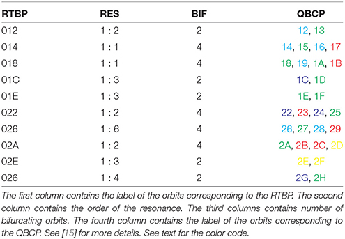
Table 2. Continuation of the low order resonant orbits from the RTBP to the QBCP.

5.3. High Order Approximation of the Unstable Manifolds of the Collinear Periodic Orbits

This section is devoted to the results of implementing the algorithm explained in section 3.2 to the dynamical equivalents of the collinear points. Figure 8 shows pieces of the stable (dashed) and unstable (solid) manifolds related to the three collinear periodic orbits (the other branches can be obtained by symmetry). From left to right: the one related to L₁, the one related to L₂ and the one related to L₃. We would like to remark that these pieces are obtained directly from the evaluation of the approximation (of order 64) of the manifolds. The error is controlled by checking that the contribution of the last term of the approximating polynomial is small. It is also checked that all the points in the pieces verify the invariance equation with high accuracy. We can observe that these approximations already give large excursions far away from the collinear points. Especially in the case of L₃, where the piece of the manifold passes very close to the triangular points. The axes of Figure 8 show the x and y values. These pieces can be mapped through the stroboscopic map to obtain larger pieces of the manifolds if it is necessary. The point of giving high order approximations of the manifold is that, just a fewer number of iterates are necessary. For the computation of the manifold related to L₃, a simple shooting method has been used. Indeed, the instability associated to this libration orbit is very weak. For the computation of the manifold related to L₂, multiple shooting is required. We have used two sections. For the computation of the manifold related to L₁, the most unstable one, we have used a single shooting strategy but with an extended precision arithmetic of 128 bits. This last approach makes the program far slower but very simple to code. In Figure 9 (left) we show the resonant orbit 2G of Table 2. We display also (right) the stable (dashed) and unstable (manifolds).

FIGURE 8

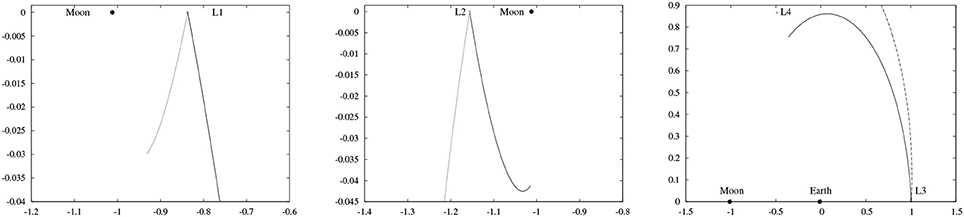
Figure 8. Approximation of order 64 of the stable (dashed) unstable (solid) manifolds of L₁, L₂ and L₃. Horizontal axis x. Vertical y.

FIGURE 9

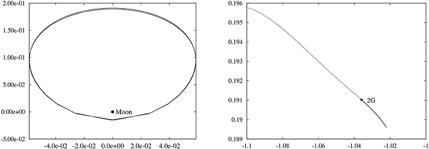
Figure 9. Left: Resonant orbit 2G. Right: Approximation of order 64 of the stable (dashed) unstable (solid) manifolds of the ressonant orbit 2G. Horizontal axis y. Vertical z.

6. Conclusions

We have presented two alternatives to the RTBP for the study of the motion of a test particle in the Earth-Moon system. Both models, the BCP and the QBCP, depend periodically on the time. We use the so-called stroboscopic map to study the minimal periodic orbits of the systems and the invariant manifolds related to them.

The BCP is as useful model for the study of the triangular points. The simplicity of the vectorfield is a strong point, especially in problems related to effective stability where massive integrations are mandatory. We have also stressed its weakness: it is not suitable to understand the dynamics around the collinear points. The BCP is useless to describe the vicinity of the translunar point.

We have used the parametrization method to obtain high order approximations of the unstable manifolds related to the minimal periodic orbits that replace the collinear points in the QBCP. This is helpful to design long excursions between the two primaries and the collinear points. The main novelty is that we have computed the manifolds directly on the stroboscopic map. The QBCP is a complicated model with a numerically computed vectorfield. This makes it a bad candidate (in front of the BCP) to be the model used to face the problems involving massive simulations related to the triangular points.

We would like to stress that the BCP should be used to face problems related to the triangular points. Especially if this problems involve large time integrations to seek for regions of practical stability. The QBCP should be used when dealing with problems involving the collinear points.

7. Technical Details

All the computations appearing in the Figures of this paper, also the ones which appear in the literature, have been performed by the authors. The integrations for the RTBP, the BCP and the QBCP have used a Taylor method with variable order and stepsize. The demanded accuracy for the standard double precision has been 10⁻¹⁶. The computations in multiple accuracy have been done using the library mpfr. The LAPACK library has also been used for some computations related to linear algebra. The rest of the programs have been written by the authors in C and C++ languages from the scratch. Table 3 and Table 4 contains the values of the parametres used for the computations.

TABLE 3

Table 3. Values of the parametres used in this paper.

TABLE 4

Table 4. Coefficients of the functions α_j, j = 1, …, 8, in (5).

Author Contributions

AF, ÀJ, and MJ-C split, more or less, equally the tasks regarding the computation and writing of the paper.

Conflict of Interest Statement

The authors declare that the research was conducted in the absence of any commercial or financial relationships that could be construed as a potential conflict of interest.

Acknowledgments

The authors would like to thank J. Gimeno and N. Miguel for their help. This work has been supported by the Spanish grants MTM2015-67724-P (MINECO/FEDER), MDM-2014-0445 and the Catalan grant 2017 SGR 1374. The project leading to this application has received funding from the European Union's Horizon 2020 research and innovation programme under the Marie Skłodowska-Curie grant agreement No 734557.

Footnotes

1. ^In principle, one could also use numerical differentiation but it is a bad approach in terms of efficiency and accuracy.

References

1. Gabern F, Jorba À, Locatelli U. On the construction of the Kolmogorov normal form for the Trojan asteroids. Nonlinearity (2005) 18:1705–34. doi: 10.1088/0951-7715/18/4/017

CrossRef Full Text | Google Scholar

2. Páez RI, Locatelli U. Trojan dynamics well approximated by a new hamiltonian normal form. arXiv:1508.00381 (2015)

Google Scholar

3. Páez RI, Efthymiopoulus C. Secondary resonances and the boundary of effective stability of trojan motions. arXiv:1712.08460 (2017)

Google Scholar

4. Gómez GG, Jorba À, Masdemont J, Simó C. A quasiperiodic solution as a substitute of l₄ in the Earth-Moon system. In: Proceedings of the 3rd International Sysmposium on Spacecraft Flight Dynamics, ESTEC. Noordwijk: ESA Publications Division (1991). p. 35–41.

Google Scholar

5. Gómez GG, Jorba À, Masdemont J, Simó C. Quasiperiodic orbits as a substitute of libration points in the solar system. In: Roy AE editor, Predictability, Stability and Chaos in N-Body Dynamical Systems. Plenum Press (1991). p. 433–438.

Google Scholar

6. Gómez GG, Jorba À, Masdemont J, Simó C. Study of Poincaré Maps for Orbits Near Lagrangian Points. ESOC contract 9711/91/D/IM(SC), final report, European Space Agency (1993). Reprinted as Dynamics and mission design near libration points. Vol. IV, Advanced methods for triangular points, volume 5 of World Scientific Monograph Series in Mathematics, (Singapore) 2001.

7. Gómez GG, Llibre J, Martínez R, Simó C. Dynamics and Mission Design Near Libration Points Vol. I, Fundamentals: The Case of Collinear Libration Points, Vol. 2, World Scientific Monograph Series in Mathematics. World Scientific Publishing Co. Inc., (2001).

8. Gómez GG, Llibre J, Martínez R, Simó C. Station Keeping of Libration Point Orbits. ESOC contract 5648/83/D/JS(SC), final report, European Space Agency (1985).

9. Huang SS. Very Restricted Four-Body Problem. NASA technical note. Washington, DC: National Aeronautics and Space Administration, (1960).

Google Scholar

10. Cronin J, Richards PB, Russell LH. Some periodic solutions of a four-body problem. Icarus (1964) 3:423–8.

Google Scholar

11. Barrabés E, Gómez G, Mondelo JM, Ollè M. Pseudo-heteroclinic connections between bicircular restricted four-body problems. Month Not R Astron Soc. (2016) 462:740–50.

Google Scholar

12. Gómez G, Jorba À, Masdemont J, Simó C. Study Refinement of Semi-Analytical Halo Orbit Theory. ESOC contract 8625/89/D/MD(SC), final report, European Space Agency (1991).

13. Castellà E, Jorba À. On the vertical families of two-dimensional tori near the triangular points of the Bicircular problem. Celestial Mech. (2000) 76:35–54. doi: 10.1023/A:1008321605028

CrossRef Full Text | Google Scholar

14. Jorba À. A numerical study on the existence of stable motions near the triangular points of the real Earth-Moon system. Astron. Astrophys. (2000) 364:327–38.

Google Scholar

15. Andreu MA. The Quasi-Bicircular Problem. PhD thesis, University of Barcelona (1998).

16. Andreu MA, Simó C. The quasi-bicircular problem for the Earth-Moon-Sun parameters. (2000). Available online at: http://www.maia.ub.es/dsg/2000/index.html

Google Scholar

17. Andreu MA. Dynamics in the center manifold around L₂ in the quasi-bicircular problem. Celestial Mech. (2002) 84:105–33. doi: 10.1023/A:1019979414586

CrossRef Full Text | Google Scholar

18. Bihan BL, Masdemont JJ, Gómez G, Lizy-Destrez S. Invariant manifolds of a non-autonomous quasi-bicircular problem computed via the parameterization method. Nonlinearity (2017) 30:3040. doi: 10.1088/1361-6544/aa7737

CrossRef Full Text | Google Scholar

19. Siegel CL, Moser JK. Lectures on Celestial Mechanics, Vol. 187 of Grundlehren der mathematischen Wissenschaften New York, NY: Springer (1971).

Google Scholar

20. Gabern F. On the Dynamics of the Trojan Asteroids. Ph.D. thesis, Universitat de Barcelona (2003).

21. Gabern F, Jorba À. A restricted four-body model for the dynamics near the Lagrangian points of the Sun-Jupiter system. Discrete Contin. Dyn. Syst. Ser. B (2001) 1:143–82. doi: 10.3934/dcdsb.2001.1.143

CrossRef Full Text | Google Scholar

22. Gabern F, Jorba À, Robutel P. On the accuracy of restricted three-body models for the Trojan motion. Discrete Contin. Dyn. Syst. Ser. B (2004) 11:843–54. doi: 10.3934/dcds.2004.11.843

CrossRef Full Text | Google Scholar

23. Szebehely V. Theory of Orbits. Orlando, FL: Academic Press (1967).

Google Scholar

24. Meyer KR, Hall GR. Introduction to Hamiltonian Dynamical Systems and the N-Body Problem. New York, NY: Springer (1992).

Google Scholar

25. Mondelo JM. Contribution to the study of Fourier methods for quasi-periodic functions and the vicinity of the collinear libration points. Ph.D. thesis, University of Barcelona (2001).

26. Farquhar RW, Kamel AA. Quasi-periodic orbits about the translunar libration point. Celest Mech. (1973) 7:458–73.

Google Scholar

27. Breakwell JV, Brown JV. The ‘halo' family of 3-dimensional periodic orbits in the earth-moon restricted 3-body problem. Celest Mech. (1979) 20:389–404.

Google Scholar

28. Celletti A, Pucacco G, Stella D. Lissajous and halo orbits in the restricted three-body problem. J Nonlinear Sci. (2015) 25:343–70.

Google Scholar

29. Gómez G, Mondelo JM. The dynamics around the collinear equilibrium points of the RTBP. Phys. D (2001) 157:283–321. doi: 10.1016/S0167-2789(01)00312-8

CrossRef Full Text | Google Scholar

30. Broucke RA. Periodic Orbits in the Restricted Three-Body Problem With Earth-Moon Masses. JPL Technical Report. Jet Propulsion Laboratory, California Institute of Technology (1968).

31. Jorba À. A methodology for the numerical computation of normal forms, centre manifolds and first integrals of Hamiltonian systems. Exp. Math. (1999) 8:155–95.

Google Scholar

32. Jorba À, Masdemont J. Nonlinear dynamics in an extended neighbourhood of the translunar equilibrium point. In: Simó C. editor. Hamiltonian Systems With Three or More Degrees of Freedom, NATO Advance Science Series C: Mathematical and Physical Science, Held in S'Agaró, Kluwer Academic Publishers, Dordrecht (1999). p. 430–434.

Google Scholar

33. Jorba À, Masdemont J. Dynamics in the centre manifold of the collinear points of the restricted three body problem. Phys. D (1999) 132:189–213.

Google Scholar

34. Haro À, de la Llave R. A parameterization method for the computation of invariant tori and their whiskers in quasiperiodic maps: numerical algorithms. Discrete Continuous Dyn Syst B (2006) 6:1261–300. doi: 10.3934/dcdsb.2006.6.1261

CrossRef Full Text

35. Haro À, de la Llave R. A parameterization method for the computation of invariant tori and their whiskers in quasiperiodic maps: numerical implementation and examples. SIAM J Appl Dyn Syst. (2005) 6:142–207. doi: 10.1137/050637327

CrossRef Full Text | Google Scholar

36. Farrés A, Jorba À. On the high order approximation of the centre manifold for ODEs. Discrete Contin. Dyn. Syst. Ser. B (2010) 14:977–1000. doi: 10.3934/dcdsb.2010.14.977

CrossRef Full Text | Google Scholar

37. Farrés A, JorbaÀ. Periodic and quasi-periodic motions of a solar sail close to SL₁ in the Earth-Sun system. Celest Mech. (2010) 107:233–253. doi: 10.1007/s10569-010-9268-4

CrossRef Full Text | Google Scholar

38. Meyer KR, Schmidt DS. The stability of the Lagrange triangular point and a theorem of Arnold. J. Diff Equat. (1986) 62:222–36.

Google Scholar

39. Arnold VI. Instability of dynamical systems with several degrees of freedom. Soviet Math. Dokl. (1964) 5:581–5.

Google Scholar

40. Giorgilli A, Delshams A, Fontich E, Galgani L, Simó C. Effective stability for a Hamiltonian system near an elliptic equilibrium point, with an application to the restricted three body problem. J. Diff Equat. (1989) 77:167–98.

Google Scholar

41. Jorba À, Villanueva J. Numerical computation of normal forms around some periodic orbits of the restricted three body problem. Phys. D (1998) 114:197–229.

Google Scholar

42. Gabern F, Jorba À. Effective computation of the dynamics around a two-dimensional torus of a Hamiltonian system. J. Nonlinear Sci. (2005) 15:159. doi: 10.1007/s00332-005-0663-z

CrossRef Full Text | Google Scholar

43. Simó C, Sousa-Silva P, Terra M. Practical stability domains near L_{4, 5} in the restricted three-body problem: Some preliminary facts. In: Santiago Ibáñez, Jesús S. Pérez del Río, Antonio Pumariño, and J. Ángel Rodríguez, editors, Progress and Challenges in Dynamical Systems Berlin; Heidelberg: Springer Berlin Heidelberg (2013). p. 367–382.

Google Scholar

44. Jorba À, Villanueva J. On the persistence of lower dimensional invariant tori under quasi-periodic perturbations. J. Nonlinear Sci. (1997) 7:427–73.

Google Scholar

45. Jorba À, Ollé M. Invariant curves near Hamiltonian-Hopf bifurcations of four-dimensional symplectic maps. Nonlinearity (2004) 17:691–710. doi: 10.1088/0951-7715/17/2/019

CrossRef Full Text | Google Scholar

46. Jorba À. Numerical computation of the normal behaviour of invariant curves of n-dimensional maps. Nonlinearity (2001) 14:943–976. doi: 10.1088/0951-7715/14/5/303

CrossRef Full Text | Google Scholar

47. Cabré X, Fontich E., de la Llave R. The parameterization method for invariant manifolds I: Manifolds associated to non-resonant subspaces. Indiana Univ. Math. J (2003) 52:283–328. doi: 10.1512/iumj.2003.52.2245

CrossRef Full Text | Google Scholar

48. Cabré X, Fontich E, de la Llave R. The parameterization method for invariant manifolds II: Regularity with respect to parameters. Ind Univ Math J. (2003) 52:329–60.

Google Scholar

49. Cabré X, Fontich E, de la Llave R. The parameterization method for invariant manifolds III: Overview and applications. J Diff Equat. (2005) 218:444–515. doi: 10.1016/j.jde.2004.12.003

CrossRef Full Text | Google Scholar

50. Simó. C. . On the analytical and numerical approximation of invariant manifolds. In: Benest D, Froeschlé C editors, Modern Methods in Celestial Mechanics. Toulouse: Frontières (1990). p. 285–330.

Google Scholar

51. Simó C, Gómez G, Jorba À, Masdemont J. The Bicircular model near the triangular libration points of the RTBP. In: Roy AE, Steves BA editors. From Newton to Chaos, New York, NY: Plenum Press. (1995). p. 343–370.

Google Scholar

52. Jorba À, Villanueva J. On the normal behaviour of partially elliptic lower dimensional tori of Hamiltonian systems. Nonlinearity (1997) 10:783–822.

Google Scholar

53. Hou XY, Xin X, Scheeres DJ, Wang J. Stable motions around triangular libration points in the real earth-moon system. Month Not R Astron Soc. (2015) 454:4172–81. doi: 10.1093/mnras/stv2216

CrossRef Full Text | Google Scholar

54. Jorba-Cuscó M, Farrés A, Jorba À. A study on the effect of solar radiation pressure on the stability region near the earth-moon triangular points. In: Proceedings of the 66th International Astronautical Congress, Jerusalem (2015). p. 12–16.

Google Scholar