 Salvador Cruz Rambaud
 Ana M. Sánchez Pérez
- Departamento de Economía y Empresa, Universidad de Almería, Almería, Spain
The framework of this paper is the field of decision-making processes in which people face the choice between probabilistic and dated rewards. Traditionally, the preferences for probabilistic outcomes have been analyzed by the Expected Utility (EU) model whilst the preferences for dated rewards have been studied by the Discounted Utility (DU) model. Nevertheless, recent empirical findings have revealed the existence of several anomalies or paradoxes in both contexts. Specifically, EU and DU models exhibit an anomaly affecting the amount of the reward, viz the “peanuts” and the magnitude effects, respectively, which seem to go in opposite directions. The aim of this paper is to analyze both effects jointly in a wide setting involving choices subject to risk and over a period of time, and thereby identify and consider the implications of one anomaly on the other.
1. Introduction
This manuscript deals with the interaction between magnitude effect and “peanuts” effect, a term used by Prelec and Loewenstein [1], Weber and Chapman [2], and Haisley et al. [3] to describe the effect of a decreasing risk-aversion with decreasing monetary rewards. This is of particular importance since these two effects move in opposite directions, and the analysis of their interactions can be useful to validate any decision-making model which takes into account the elements of time and risk. The first part of the paper considers some implications of peanuts effect, magnitude effect, subendurance, and their reverse versions. The second part of the paper focuses on discount functions V given by the product of a utility function u and a function g depending on p and t, and goes on to analyze the implications which the magnitude effect and peanuts effect have on the utility function u.
Individual decision-making has been studied within disciplines which range from economics to psychology, passing through areas such as neuroscience [4]. However, these studies have always been carried out using two principal models:
1. The Discounted Utility (DU) model which is employed to assess a stream of rewards with different maturities [5]. In this way, individuals try to maximize their discounted payoff or “utility” which is given by:
where U0 is the present value of the sequence, ut is the utility obtained from the outcome available at instant t (t = 1, 2, …, T) and δ represents the discount factor (which is lower than or equal to 1).
2. The Expected Utility (EU) theory which is employed to model those decision processes involving risky choices [6], that is to say, when the amounts have been specified in terms of probability. In the same way, individuals try to maximize their expected utility:
where U0 is the present value of the experience, uk the utility obtained from the k-th experience and pk the probability associated with this experience (where obviously the n associated probabilities amount to 1: ).
The DU and EU models have a similar structure given that they are based on the same theoretical principles, since alternatives are assessed by taking into account the sum of their utilities [7]. Moreover, DU and EU are general models with the power to predict, and their high level of acceptance is explained by their simplicity and the fact that they are based on the traditional systems of calculation of the present and actuarial values, respectively.
Nowadays, the DU and EU models are the standard theories of rational choice over time and under risk, respectively, in many social and behavioral sciences [8]. However, it is well known that models are simplified representations of reality, and so this is a limitation when trying to describe the actual behavior of people [9]. In effect, several anomalies have recently been detected which must be taken into account when analyzing a real situation.
Despite their similarity, decisions involving intertemporal choices and uncertainty have traditionally been studied in different research areas, given that delayed and risky rewards do not require the same treatment. Some cautious attempts to integrate DU and EU models, such as the Discounted Expected Utility (DEU) [10, 11], have been made in order to analyze individual behavior in decisions involving time delay and risk [11, 12]. In the same vein, in psychology, it is usual to interpret time in a probabilistic way [13], or to translate risks into delays when facing risky choices [14].
Other scholars [1, 7, 15] have studied the analogies and the anomalies observed in DU and EU models by arguing that they start from certain fundamental psychological properties of multidimensional prospect valuation. In the following paragraph, some anomalies of the DU (intertemporal choices) and EU (risky choices) models are jointly presented:
1. The common difference effect (DU anomaly) and the common ratio effect (EU anomaly) [1].
2. The immediacy effect (DU anomaly) and the certainty effect (EU anomaly) [16].
3. The magnitude effect (DU anomaly) and the peanuts effect (EU anomaly).
In spite of the fact that the magnitude and the peanuts effects are embedded in different frameworks, intuitively they seem to move in opposite ways because “the peanuts effect seems to reveal decreasing sensitivity to payoffs at larger stakes, while the magnitude effect seems to reveal increasing sensitivity to payoffs at large stakes” [11]. In effect, whilst the magnitude effect occurs in the DU model, the peanuts effect makes sense in the EU model. For this reason, in this paper we will follow a joint model in which time and risk preferences are integrated, in the same line as Schneider [11] and Baucells and Heukamp [17].
In this paper, we will focus on the study of the magnitude effect and its relation with the peanuts effect both depending on the amounts of reward. The importance of this research is obvious: “Prelec and Loewenstein could not explain both effects, and this challenge has remained unresolved over the subsequent twenty-five years, posing an apparent impossibility result that no common approach to modeling risk and time preferences can capture both of these basic behaviors” [11].
The DU and EU models propose that relative preference between two options is consistent, even if their amounts of reward are increased by a constant factor [18, 19]. However, some authors [20–23] have demonstrated that in decisions with delayed rewards, the preference increases as its amount increases. This magnitude effect is based on the premise that the patience of individuals is directly related to the reward amount and that individuals are more patient for large rewards than for those of smaller amounts, leading to an increased preference for the larger later outcomes [24, 25]. Following Schneider [11], the magnitude effect may be represented as follows:
where x < y, s < t and k > 1, where p represents the probability of occurrence which is considered constant in both alternatives. This paradox explains how large outcomes are discounted at a lower rate than smaller ones, the discount rate being a decreasing function of the size of the reward [7].
On the other hand, in choices involving risk, the amount of the reward has the opposite effect on the decision-making process. As pointed out by some scholars [26, 27], the peanuts effect has not yet been addressed as thoroughly as the magnitude effect. Only some recent studies [11] have mathematically analyzed this effect. It may be defined as follows (x < y):
the probabilities of occurrence being p and q, with p > q, and k > 1. Another definition of the peanuts effect was provided by Schneider and Day [28], as follows. Consider a lottery f :(x, p; 0, 1 − p), with x > 0. Let c := {f, E(f)}. Then, the peanuts effect holds if f ≻c E(f), for sufficiently small x, and E(f) ≻c f, for sufficiently large x, for every p ∈ (0, 1).
Weber and Chapman [2] revealed that “a utility function cannot account for the decrease in the size of the peanuts effect for smaller probabilities”. In the same way, Schneider and Day [28] proved that the peanuts effect cannot hold for Cumulative Prospect Theory (CPT) or any non-choice-set-dependent EU model. Finally, Leland and Schneider [8] define the indifference relationship in the framework of the so-called Salience Weighted Utility over Presentations (SWUP) model in the following way:
and the preference relationship by the following inequality:
where μ(x, y) and π(s, t) are the so-called “salience functions”. In this way, they characterize the magnitude and the peanuts effects by imposing some conditions on the utility and the salience functions.
As indicated in the previous paragraphs, the magnitude and peanuts effects seem to move in opposite directions, and can be explained by two a priori psychological principles:
1. The magnitude effect may be explained by the psychology of perception, where individuals are more sensitive to absolute than to relative differences in magnitude [1, 29]. It should be borne in mind that decision-makers see larger delayed rewards as investments. In this way, the potential of earning a bigger amount of money leads to choosing the delayed reward with its corresponding increase.
2. The risk-seeking in the peanuts effect may be explained by the anticipated emotion of disappointment [16]. Disappointment is an emotion which is experienced when perceiving that a different situation would have led to a better result [30]. As some scholars [31, 32] suggest, the effect of anticipated emotions may influence individual decisions. According to the perceived level of this disappointment, the utility is a function of the difference between the actual outcome and the expected value of the gamble. In order to avoid the feeling of disappointment, a person prefers a less risky gamble over a riskier one. Because of this, the decision-maker becomes risk-seeking for potential smaller rewards given that losing them invokes less disappointment than losing a bigger one.
The influence of negative emotion is likely to be greater in risky choice than in intertemporal choice because the possibility of gaining a reward smaller than expected is implicit in risky choices. The presented studies confirm that, from a psychological point of view, probabilistic discounting is not identical to that which underlies temporal discounting.
The methodology employed in this paper is the interaction between time and risk preferences. Its main contribution is the way by which time and risk preferences interact given certain assumptions. As a result, a wide variety of mathematical relationships arise by using the concepts of regularity and subendurance, and an important representation of the discount function V(x, p, t) as u(x)g(p, t).
After describing the state of the art concerning the mathematical treatment in the existing literature of both the magnitude and the peanuts effects, this paper is organized as follows. In section 2, the possible relationships between the magnitude and the peanuts effects are analyzed by using a very general definition of discount function involving time delay and risk, and the presence or absence of the so-called subendurance. In section 3, the general expression of the discount function V(x, p, t) is restricted to the functional form u(x)g(p, t), where u is a utility function. Under these circumstances, some significant relationships can be obtained between the reverse magnitude and the peanuts effects in the presence of a regular discount function. Finally, section 4 summarizes and concludes.
2. Framework and General Results
2.1. Preliminaries
It will prove useful to begin with some definitions [17].
Definition 1. Consider the set , where X = [0, +∞), P = [0, 1], and T = [0, +∞). A discount function is a continuous real-valued function V(x, p, t) defined on which is strictly increasing in the first and second components, and strictly decreasing in the third.
However, Baucells and Heukamp [17] require that V tends to zero whenever xpe − t tends to zero, but in this paper this restriction will be relaxed, and we will assume that V converges to zero only when x → 0 or p → 0, by allowing that
In the first case, V is said to be regular whilst, if L(x, p) > 0, V is said to be singular. The paper by Baucells and Heukamp [17] implicitly includes the regularity of V. In some further results we will require this condition but in others this condition will not be necessary. The following definitions have been obtained from Schneider [11].
Definition 2. The peanuts effect (resp. reverse peanuts effect) is said to hold if, for every 0 < x < y, p > q and k > 1, (x, p, t) ~ (y, q, t) implies (kx, p, t) ≻ (ky, q, t) (resp. (kx, p, t) ≺ (ky, q, t)).
Definition 3. The magnitude effect (resp. reverse magnitude effect) is said to hold if, for every 0 < x < y, s < t and k > 1, (x, p, s) ~ (y, p, t) implies (kx, p, s) ≺ (ky, p, t) (resp. (kx, p, s) ≻ (ky, p, t)).
The following definition reflects the idea that the larger the reward, the more subjects are willing to wait in exchange for improved probabilities [17].
Definition 4. Subendurance (resp. reverse subendurance) is said to hold if, for every 0 < x < y, s < t and p < q, (y, p, s) ~ (y, q, t) implies (x, p, s) ≻ (x, q, t) (resp. (x, p, s) ≺ (x, q, t)).
2.2. General Results
Lemma 1. Given an x ∈ X, let Vx : P × T → ℝ be the real function defined by Vx(p, t) := V(x, p, t). If V is regular, then, for every (p, t) ∈ P × T and every q > p, there exists a Δ = Δ(x, p, q, t) > 0 such that Vx(q, t + Δ) = Vx(p, t).
Proof. Given an x ∈ X, for every (p, t) ∈ P × T and every q > p, let us consider the following real-valued function:
defined as:
Taking into account the definition of V, the inequality Vx,q(t) > Vx(p, t) holds. Moreover, as V is regular, when r → +∞, Vx,q(r) → 0. Therefore, there exists a r0, large enough, such that Vx,q(r0) ≤ Vx(p, t) < Vx,q(t). As V is continuous and decreasing in t, by the Intermediate Value Theorem there exists a value Δ > 0 such that Vx,q(t + Δ) = Vx(p, t), from where Vx(q, t + Δ) = Vx(p, t).□
Corollary 1. Let Vp : X × T → ℝ be the real function defined by Vp(x, t) := V(x, p, t). If V is regular, then, for every (x, t) ∈ X × T and every y > x, there exists a Δ = Δ(x, y, p, t) > 0 such that Vp(y, t + Δ) = Vp(x, t).
Proof. The proof is analogous to that of Lemma 1 because the amount x and the probability p play similar rôles.□
Observe that the next two results do not require the condition of regularity of V.
Lemma 2. Let Vt : X × P → ℝ be the real function defined by Vt(x, p) := V(x, p, t). For every (x, p) ∈ X × P and every q > p, there exists a 0 < k = k(x, p, q, t) < 1 such that Vt(kx, q) = Vt(x, p).
Proof. Given a t ∈ T, for every (x, p) ∈ X × P and every q > p, let us consider the following real-valued function:
defined as:
Taking into account the definition of V, the inequality Vq,t(x) > Vt(x, p) holds. Moreover, as Vq,t(0) = 0, then Vq,t(0) ≤ Vt(x, p) < Vq,t(x). As V is continuous and increasing in x, by the Intermediate Value Theorem there exists a value 0 < k = k(x, p, q, t) < 1 such that Vq,t(kx) = Vt(x, p), from where Vt(kx, q) = Vt(x, p).□
Corollary 2. Let Vt : X × P → ℝ be the real function defined by Vt(x, p) := V(x, p, t). For every (x, p) ∈ X × P and every y > x, there exists a 0 < k = k(x, p, q, t) < 1 such that Vt(y, kp) = Vt(x, p).
Proof. The proof is analogous to that of Lemma 1 because the amount x and the probability p play similar rôles.□
Observation 1. It can be shown that the peanuts effect holds if and only if, for every 0 < x < y, p > q and 0 < h < 1, (x, p, t) ~ (y, q, t) implies (hx, p, t) ≺ (hy, q, t). In effect, assume that (x, p, t) ~ (y, q, t), with 0 < x < y and p > q. If, for a given 0 < h < 1, (hx, p, t) ≽ (hy, q, t), then Vp,t(0) ≤ V(hy, q, t) ≤ Vp,t(hx). As Vp,t is continuous and increasing, by the Intermediate Value Theorem, there would be a h0 ≤ h such that (h0x, p, t) ~ (hy, q, t). As 1/h0 > 1, by hypothesis,
which is a contradiction. Therefore, (hx, p, t) ≺ (hy, q, t). The proof of the reciprocal implication is analogous.
Observation 2. Analogously to Observation 1, it can be shown that the magnitude effect holds if and only if, for every 0 < x < y, s < t and 0 < h < 1, (x, p, s) ~ (y, p, t) implies (hx, p, s) ≻ (hy, p, t).
Observation 3. Finally, observe that it can be shown that subendurance holds if and only if, for every 0 < x < y, s < t and p < q, (x, p, s) ~ (x, q, t) implies (y, p, s) ≺ (y, q, t). The proof is analogous to that of observations 1 and 2.
Theorem 1. The magnitude and the peanuts effects imply subendurance.
Proof. In effect, assume that the magnitude and the peanuts effects hold. In order to show that subendurance is satisfied, we are going to start from the following indifference relation:
where s < t, and p < q. By Lemma 2, there is a “trade-off” between y and q, in the way that the amount y can be increased until z, in exchange for diminishing the probability up to the value p, keeping the former indifference between the involved rewards, that is to say, such that:
where z > y. Therefore, as the magnitude effect holds, one has:
with k > 1. On the other hand, we can apply transitivity to equivalences (5) and (6), and so derive that:
By applying now the peanuts effect to the former equivalence and for the same value of k, one has:
Finally, the transitivity applied again to preferences (7) and (9) results in:
from where subendurance holds (see Observation 3).□
Theorem 2. The following statements hold1:
1. The magnitude effect and the reverse subendurance imply the reverse peanuts effect.
2. The reverse magnitude effect and the subendurance imply the peanuts effect.
3. The reverse magnitude effect and the reverse peanuts effect imply the reverse subendurance.
4. The peanuts effect and the reverse subendurance imply the reverse magnitude effect.
5. The reverse peanuts effect and the subendurance imply the magnitude effect.
Proof. The proof is analogous to that of Theorem 1.□
All the implications included in theorems 1 and 2 can be schematized in Figure 12. Observe that:
1. Only in the context of subendurance, the magnitude and the peanuts effects are compatible. That is to say, in the context of reverse subendurance, these effects are incompatible.
2. In both contexts (subendurante and reverse subendurance), there are some implications of the magnitude for the reverse peanuts effects, and of the reverse magnitude for the peanuts effects.
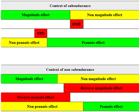
Figure 1. Implications between the magnitude and the peanuts effects. Green denotes de presence of the mentioned effect. Yellow denotes de absence of the indicated effect. Red represents the existence of the reverse of the mentioned effect. Source: own elaboration.
3. Searching Particular Implications
3.1. Introducing a Discount Function
Assume that the discount function has the functional form V(x, p, t) := u(x)g(p, t), where u is a utility function and g(p, t) is a non-negative continuous function defined in P × [0, t0) (t0 can even be +∞, in which case [0, t0) = T) satisfying the following conditions:
1. g(p, t) > 0.
2. g(p, t) is increasing with respect to p, and
3. g(p, t) is decreasing with respect to t.
The discount function is said to be [33]
1. Regular if t0 = +∞ and , for every p ∈ P (see Figure 2).
2. Singular if t0 = +∞ and , for some p ∈ P (see Figure 3).
3. With bounded domain if t0 ∈ ℝ.
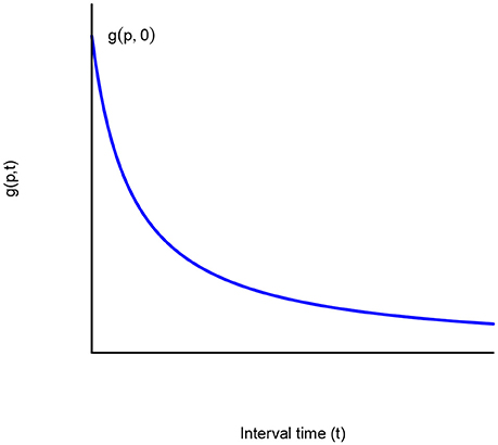
Figure 2. A regular discount function. Source: own elaboration.
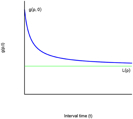
Figure 3. A singular discount function. Source: own elaboration.
3.2. Particular Results
According to Baucells and Heukamp [17], this model is not compatible with subendurance and reverse subendurance. In these conditions, we can put forward the following propositions.
Proposition 1. A sufficient condition for the magnitude effect (resp. reverse magnitude effect) is that, for every 0 < x < y, s < t, p ≥ q and k > 1, (x, p, s) ~ (y, q, t) implies (kx, p, s) ≺ (ky, q, t) (resp. (kx, p, s) ≻ (ky, q, t)). If V is regular, this condition is also necessary.
Proof. Obviously, the condition is sufficient (it suffices to take p = q). Let us see the necessity. In effect, assume that the magnitude effect holds. In order to show that the aforementioned condition holds, we are going to start from the following indifference relation:
where 0 < x < y, s < t and p ≥ q. From the former equivalence, it can be deduced that
By Lemma 1, the next step is to propose a “trade-off” between q and t, in the way that the instant t can be delayed until t′, in exchange for increasing the probability up to p, keeping the indifference between the involved rewards, that is to say, such that:
In effect, it suffices to define (taking into account that g(p, ·) is continuous and decreasing)
The existence of such t′ is guaranteed because V is regular. Therefore, as the magnitude effect holds, one has:
for every k > 1.
Finally, observe that, from the former equalities and inequalities, the following inequality is satisfied:
which obviously derives in:
and so the condition is necessary. The reasoning for the reverse magnitude effect is analogous.□
Proposition 2. The peanuts effect (resp. reverse peanuts effect) holds if and only if, for every 0 < x < y, s ≤ t, p > q and k > 1, (x, p, s) ~ (y, q, t) implies (kx, p, s) ≻ (ky, q, t) (resp. (kx, p, s) ≺ (ky, q, t)).
Proof. Obviously, the condition is sufficient (it suffices to take s = t). Let us see the necessity. In effect, assume that the peanuts effect holds. In order to show that the aforementioned condition holds, we are going to start from the following indifference relation:
where 0 < x < y, s ≤ t and p > q. From the former equivalence, it can be deduced that
The next step is to propose a “trade-off” between q and t, in the way that the probability q can be reduced until q′, in exchange for anticipating the availability of the second reward up to s, keeping the indifference between the involved rewards, that is to say, such that:
In effect, it suffices to define (taking into account that g(·, s) is continuous and decreasing, and g(0, s) = 0)
Therefore, as the peanuts effect holds, one has:
for every k > 1.
However, observe that, from the former equalities and inequalities, the following inequality is satisfied:
which obviously derives in:
and so the condition is necessary. The reasoning for the reverse peanuts effect is analogous.□
The following results are a direct consequence of propositions 1 and 2 in the framework defined at the beginning of section 3.
Corollary 3. The peanuts effect implies the reverse magnitude effect. Moreover, if the discount function involved in the intertemporal choice is regular, then the reverse magnitude effect implies the peanuts effect.□
Corollary 4. If the model involved in the intertemporal choice is the q-exponential discounting, then the reverse magnitude effect is equivalent to the peanuts effect.
Proof. In effect, take into account that the q-exponential (in particular, the exponential, the hyperbolic and the linear discounting) discount function [34] is regular, as required by Corollary 3.□
The following proposition provides a characterization of the utility function u involved in the context of the peanuts effect.
Proposition 3. The peanuts effect holds if and only if the elasticity of the utility function
is decreasing.
Proof. Let us assume that the peanuts effect holds and that 0 < x < y. Let p and q (p > q) be two probabilities such that (x, p, t) ~ (y, q, t). In such a case,
By the peanuts effect, (kx, p, t) ≻ (ky, q, t) for every k > 1, and so
By dividing the left and the right-hand sides of the former expressions, one has:
and so
As k > 1, we can write k := 1+h, with h > 0. Therefore,
Dividing both sides of the former inequality by h and letting h → 0, we obtain:
Consequently, the elasticity of the utility function, z[ln u(z)]′, is decreasing. The converse implication can be easily shown.□
This result coincides with that provided by [35].
Corollary 5. If the peanuts effect holds then u is ln-concave.
Proof. In effect, if the peanuts effect holds, by Proposition 3, z[ln u(z)]′ is decreasing. As z is increasing, then [ln u(z)]′ is decreasing. Therefore, u is ln-concave.□
The converse statement is not true. In effect, the utility function is ln-concave (see Figure 4, line in blue) but
is increasing (see Figure 4, line in green).

Figure 4. Counterexample of corollary 5. Source: own elaboration.
Analogously, we can show the following statements.
Proposition 4. The magnitude effect holds if and only if the elasticity of the utility function is increasing.□
Corollary 6. If u is ln-convex then the magnitude effect holds.□
All the implications between the analyzed effects and the ln-convexity of u can be seen in Figure 5.
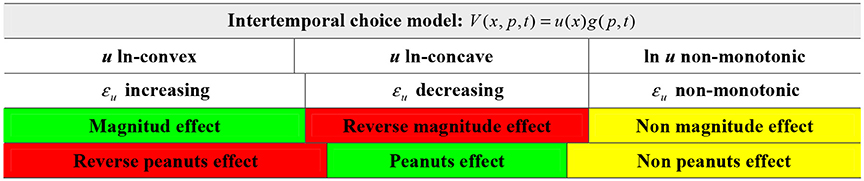
Figure 5. Convexity, and peanuts and magnitude effects Green denotes de presence of the mentioned effect. Yellow denotes de absence of the indicated effect. Red represents the existence of the reverse of the mentioned effect. Source: own elaboration.
4. Conclusions
In behavioral finance, the decision-making processes should be explained through appropriate theoretical models and taking into account the possible anomalies that human behaviors entail. The treatment of these paradoxes can improve the explanatory power of the economic models by involving some suitable tools from the fields of economics and psychology.
Although sometimes time and risky preferences may be considered as analogous concepts, the temporal and probabilistic discount functions are not identical. To illustrate the difference between intertemporal and probabilistic choices, we refer to two anomalies of the discounted and expected utility models: the magnitude and the peanuts effects, respectively.
The magnitude effect occurs in intertemporal choices where the larger reward is usually related to a longer waiting time and a lower discount rate. Given that these choices occur free of negative feelings such as disappointment, the decision-maker, in search of greater profits, may prefer to wait. However, the peanuts effect occurs in uncertain choices in which the disappointment experienced is directly related to the amount and probability of the result. Specifically, the decision-maker is more prone to make risky decisions when a small amount is involved in the experiment.
This paper has presented a model simultaneously applied to time and risk which could explain both the magnitude effect in choices over time and the peanuts effect in choices under risk. In pursuit of establishing the relationship between both effects, we have obtained some implications in a broad framework by considering the presence or absence of subendurance. In the particular case in which V(x, p, t) adopts the expression u(x)g(p, t), where u is a utility function, the reverse magnitude and the peanuts effects are equivalent when the discount function is regular. Finally, some implications have been deduced involving the ln-convexity of u(x).
Author contributions
SC and AS contributed to the design and implementation of the research, and to the writing of the manuscript.
Funding
The authors gratefully acknowledge financial support from the Spanish Ministry of Economy and Competitiveness [National R&D Project DER2016-76053-R].
Conflict of interest statement
The authors declare that the research was conducted in the absence of any commercial or financial relationships that could be construed as a potential conflict of interest.
Acknowledgments
We are very grateful for the valuable comments and suggestions offered by two referees.
Footnotes
1. ^The additional condition of the discount function being regular will be taken into account when a trade-off between reward amount (or probability) and time is necessary in order to apply Lemma 1 and Corollary 1.
2. ^In order to interpret this chart and the next one correctly, it is necessary to take into account the following criterium: if a cell can be vertically embedded in a contiguous cell, the property indicated in the first (smaller) cell implies the property enclosed in the second (bigger) cell.
References
1. Prelec D, Loewenstein G. Decision making over time and under uncertainty: a common approach. Manag Sci. (1991) 37:770–86. doi: 10.1287/mnsc.37.7.770
2. Weber BJ, Chapman GB. Playing for peanuts: why is risk seeking more common for low-stakes gambles? Organ Behav Hum Decis Process. (2005) 97:31–46. doi: 10.1016/j.obhdp.2005.03.001
3. Haisley E, Mostafa R, Loewenstein G. Myopic risk-seeking: the impact of narrow decision bracketing on lottery play. J Risk Uncertain. (2008) 37:57–75. doi: 10.1007/s11166-008-9041-1
4. Berns GS, Laibson D, Loewenstein G. Intertemporal choice-toward an integrative framework. Trends Cogn Sci. (2007) 11:482–8. doi: 10.1016/j.tics.2007.08.011
5. Samuelson PA. A note on measurement of utility. Rev Econ Stud. (1937) 4:155–61. doi: 10.2307/2967612
6. Von Neumann J, Morgenstern O. Theory of Games and Economic Behavior. Princeton, NJ: Princeton University Press (1947).
7. Baucells M, Heukamp FH, Villasís A. Risk and time preferences integrated. In: Foundations of Utility and Risk Conference. Rome (2006).
8. Leland J, Schneider M. Risk preference, time preference, and salience perception. In: ESI Working Papers 17–16, Orange, CA (2017). Available online at: http://digitalcommons.chapman.edu/esi_working_papers/228/
9. Schoemaker PJ. The expected utility model: its variants, purposes, evidence and limitations. J Econ Lit. (1982) 20:529–63.
10. Andreoni J, Sprenger C. Risk Preferences Are Not Time Preferences: Discounted Expected Utility With a Disproportionate Preference for Certainty. Cambridge, MA: National Bureau of Economic Research (2010).
11. Schneider M. Dual-process utility theory: a model of decisions under risk and over time. In: ESI Working Paper 16-23, Orange, CA (2016). Available online at: http://digitalcommons.chapman.edu/esi_working_papers/201
13. Keren G, Roelofsma P. Immediacy and certainty in intertemporal choice. Organ Behav Hum Decis Process. (1995) 63:287–97. doi: 10.1006/obhd.1995.1080
14. Rachlin H, Raineri A, Cross D. Subjective probability and delay. J Exp Anal Behav. (1991) 55:233–44. doi: 10.1901/jeab.1991.55-233
15. Quiggin J, Horowitz J. Time and risk. J Risk Uncertain. (2012) 10:37–55. doi: 10.1007/BF01211527
16. Weber BJ, Chapman GB. The combined effects of risk and time on choice: Does uncertainty eliminate the immediacy effect? Does delay eliminate the certainty effect? Organ Behav Hum Decis Process. (2005) 96:104–18. doi: 10.1016/j.obhdp.2005.01.001
17. Baucells M, Heukamp FH. Probability and time trade-off. Manag Sci. (2012) 4:831–42. doi: 10.1287/mnsc.1110.1450
18. Suzuki S. Negative emotion or problem content? Testing explanations of the peanuts effect. Psychol Rep. (2015) 116:1–12. doi: 10.2466/15.04.PR0.116k15w5
19. Kahneman D, Tversky A. Prospect theory: an analysis of decision under risk. Econometrica (1979) 47:263–91. doi: 10.2307/1914185
20. Green L, Myerson J, McFadden. Rate of temporal discounting decreases with amount of reward. Mem Cogn. (1997) 25:715–23. doi: 10.3758/BF03211314
21. Kirby KN. Bidding on the future: Evidence against normative discounting of delayed rewards. J Exp Psychol Gen. (1997) 126:54–70. doi: 10.1037/0096-3445.126.1.54
22. Chapman GB, Winquist JR. The magnitude effect: temporal discount rates and restaurant tips. Psychon Bull Rev. (1998) 5:119–23. doi: 10.3758/BF03209466
23. Grace RC, McLean AP. Integrated versus segregated accounting and the magnitude effect in temporal discounting. Psychon Bull Rev. (2005) 12:732–9. doi: 10.3758/BF03196765
24. Luckman A, Donkin C, Newell BR. People wait longer when the alternative is risky: The relation between preferences in risky and intertemporal choice. J Behav Decis Making. (2017) 30:1078–92. doi: 10.1002/bdm.2025
25. Vanderveldt A, Green L, Rachlin H. Discounting by probabilistic waiting. J Behav Decis Making. (2017) 30:39–53. doi: 10.1002/bdm.1917
26. Hershey JC, Schoemaker PJH. Prospect theory's reflection hypothesis: A critical examination. Organ Behav Hum Perform. (1980) 25:395–418. doi: 10.1016/0030-5073(80)90037-9
27. Chapman GB, Weber BJ. Decision biases in intertemporal choice and choice under uncertainty: testing a common account. Mem Cogn. (2006) 34:589–602. doi: 10.3758/BF03193582
28. Schneider M, Day R. Target-adjusted utility functions and expected-utility paradoxes. Manag Sci. (2018) 64:271–87. doi: 10.1287/mnsc.2016.2588
29. Read D, Loewenstein G. Time and decision: introduction to the special issue. J Behav Decis Making. (2000) 13:141. doi: 10.1002/(SICI)1099-0771(200004/06)13:2<141::AID-BDM347>3.0.CO;2-U
30. Zeelenberg M, Van Dijk WW, Manstead AS, vanr de Pligt J. On bad decisions and disconfirmed expectancies: the psychology of regret and disappointment. Cogn Emotion. (2000) 14:521–41. doi: 10.1080/026999300402781
31. Perugini M, Bagozzi RP. The distinction between desires and intentions. Eur J Soc Psychol. (2004) 34:69–84. doi: 10.1002/ejsp.186
32. Lindsey LLM, Yun KA, Hill JB. Anticipated guilt as motivation to help unknown others: an examination of empathy as a moderator. Commun Res. (2007) 34:468–80. doi: 10.1177/0093650207302789
33. Cruz Rambaud S, Muñoz Torrecillas MJ. Some characterizations of (strongly) subadditive discounting functions. Appl Math Comput. (2014) 243:368–78. doi: 10.1016/j.amc.2014.05.095
34. Takahashi T, Han R, Nakamura F. Time discounting: psychophysics of intertemporal and probabilistic choices. J Behav Econ Finance (2012) 5:10–4. doi: 10.11167/jbef.5.10
Keywords: intertemporal choice, discounted utility model, expected utility model, magnitude effect, “peanuts” effect
Citation: Cruz Rambaud S and Sánchez Pérez AM (2018) The Magnitude and “Peanuts” Effects: Searching Implications. Front. Appl. Math. Stat. 4:36. doi: 10.3389/fams.2018.00036
Received: 05 May 2018; Accepted: 18 July 2018;
Published: 17 August 2018.
Edited by:
Sergio Ortobelli Lozza, University of Bergamo, ItalyReviewed by:
Alessandro Staino, University of Calabria, ItalySimon Grima, University of Malta, Malta
Copyright © 2018 Cruz Rambaud and Sánchez Pérez. This is an open-access article distributed under the terms of the Creative Commons Attribution License (CC BY). The use, distribution or reproduction in other forums is permitted, provided the original author(s) and the copyright owner(s) are credited and that the original publication in this journal is cited, in accordance with accepted academic practice. No use, distribution or reproduction is permitted which does not comply with these terms.
*Correspondence: Ana M. Sánchez Pérez, YW1zYW5jaGV6QHVhbC5lcw==