Analytic Quantification of Shilnikov Chaos in Epileptic EEG Data

1. Introduction

Dimensionality reduction of time-series data is often obtained by statistical methods, like principal component analysis (PCA) [1] or independent component analysis (ICA) [2]. As these methods rely on statistical model assumptions, they are not optimal for settings, were deterministic dynamics govern the signal.

Dynamical Systems Based Modeling (DSBM) [3] is a method integrating a deterministic model assumption into the dimensionality reduction process. This approach is very useful in situations where one has higher-dimensional sensor data than modeling approaches, describing the underlying system, use. A typical example for this situation is EEG data where one has many (≥25) sensors but typical models only have three to five state variables. Especially during absences the correlation dimension, an intrinsic measure for the dimensionality of the time-series data, drops to the value of three.

The existence of homoclinic Shilnikov chaos in theoretical models for epileptic EEG data was shown in van Veen and Liley [4] using bifurcation analysis. Asides the Shilnikov attractor is O(3)-invariant [5], a property which every EEG-model should posess, as the choice of the reference electrode is somewhat arbitrary. Former investigations [6, 7] have indicated the existence of Shilnikov chaos in petit-mal epilepsies, as well.

To rigorously show the existence of homoclinic Shilnikov chaos in EEG data of epileptic absences, we need on one hand a projection onto a three-dimensional space and estimation of the parameters of a system of ordinary differential equations (ODEs). This is achieved using DSBM. On the other hand, one needs to show that the system of ODEs does exhibit homoclinic Shilnikov chaos. This is done using linear stability analysis, based on the Hartman-Grobman and the Shilnikov theorem.

In this study it is not our primary intention to provide an algorithm for seizure detection or seizure prediction, which are often data-driven, like e.g., [8, 9], and in the case of prediction often fail, see e.g., [10]. Our goal is to project the high-dimensional signal onto a low-dimensional set of ODEs and to investigate the quality of the projection in the ictal and interictal periods and to compare the obtained models. A low-dimensional description of epileptic seizures yield further insight in the underlying processes and may help to improve the treatment of epilepsy patients.

The structure of the paper is as follows. In section 2.1 the DSBM procedure is presented. Linear stability analysis and quantification of Shilnikov chaos is recalled in section 2.2. A description of the data used can be found in section 2.3 and the evaluation of the results is illustrated in section 3. Finally we discuss the results in section 4.

2. Materials and Methods

2.1. Dynamical Systems Based Modeling

Dynamical Systems Based Modeling is a methodology to simultaneously estimate the parameters of a system of ordinary differential equations from data and reduce the dimensionality of the data. Assume we want to estimate the parameters a_i of a system of ordinary differential equations

$\begin{array}{rc}{ẋ}_i=a_i^{\top }{\xi }_i(x_1,\dots ,x_n),i=1,\dots ,n& (1)\end{array}$

where ξ_i is a set of basis functions as model assumption. A typical ansatz for estimating the parameters a_i would be to solve a normalized least-squares problem

$\begin{array}{rc}{\displaystyle \underset{a_i}{min}}{\displaystyle \sum _{i=1}^n}\frac{{\langle {({ṡ}_i-a_i^{\top }{\xi }_i)}^2\rangle }_t}{{\langle {ṡ}_i^2\rangle }_t},& (2)\end{array}$

where 〈·〉_t denotes the average over the time sample points t = 1, …, T and ṡ_i are the derivatives of the samples.

Now consider that we have signal data sampled in a high-dimensional space q(t)∈ℝ^N, with n≪N. Then the approach (2) is not applicable, since the samples q have dimension N≫n. Hence one has to choose a projection P∈ℝ^{n × N} to project the sampled signal to a subspace of dimension n. In Uhl et al. [3] it was shown that the cost function to minimize

$\begin{array}{rc}D(P,a)={\displaystyle \sum _{i=1}^n}\frac{{\langle {({ẏ}_i-a_i^{\top }{\xi }_i)}^2\rangle }_t}{{\langle {ẏ}_i^2\rangle }_t},\text{\hspace{1em}with}{y}_i={(Pq)}_i& (3)\end{array}$

actually depends on the projection P only D(P, a) = D(P). Hence it suffices to minimize D(P) on the set of all projections

$\begin{array}{rc}P={\displaystyle \underset{P\in {ℝ}^{n\times N}}{argmin}}D(P).& (4)\end{array}$

Note that D(P) is bounded by n from above, as can easily be seen by setting a_i = 0 for all i. If the minimal value of D(P, a) is diveded by n, it represents the relative error of the model representing the dynamics of the projection.

If the basis functions ξ_i are polynomials one can show [11] that the cost function depends on the subspace on which to project, only. Hence we actually consider a cost function on a Grassmannian manifold. Recall that a Grassmannian manifold Gr(n, N) is the set of all n-dimensional linear subspaces of ℝ^N. There are various possibilities to represent this manifold. For example one could identify the Grassmannian with a homogeneous space [12] or with the set of rank n symmetric, projection operators on ℝ^N [13]. We identify the Grassmannian with equivalence classes [P] of matrices P∈ℝ^{N × n} of rank n, where two such matrices P₁ and P₂ are equivalent if their coimages are equal coim(P₁) = coim(P₂). That is, two matrices $P_1,P_2\in {ℝ}^{N\times n}$ are identified if all the principal angles between subspaces of ℝ^N spanned by the column of the matrices are zero.

We want to find a global minimum of the cost function. For the global optimization we use a MultiStart algorithm, which generates many starting points, runs local optimization methods on each starting point and then chooses the optimum of the found local optima. As local optimization method we use a Levenberg-Marquardt algorithm [14], which solves the least-squares problem

$\begin{array}{cc}\underset{x\in {ℝ}^m}{\min }{\Vert f(x)\Vert }_2^2& (5)\end{array}$

for a non-linear function f:ℝ^m → ℝⁿ with m < n. To show that one can apply the Levenberg-Marquardt algorithm, we have to rewrite the cost function as follows. Denote by Q_i = 〈_{ξi ⊗ ξi 〉 t} the dyadic product of the basis vectors, describing the auto-correlation of the basis, and by $b_i={\langle {\stackrel{·}{Pq}}_i{\xi }_i\rangle }_t$ the componentwise product of the time derivative of the projected signal with the basis functions, describing the correlation between the derivative of the data with the basis vectors. Then by a variational calculus argument it can be shown [3] that

$\begin{array}{rc}D(P)={\displaystyle \sum _{i=1}^n}\frac{{\langle {({ẏ}_i-Q_i^{-1}{b}_i{\xi }_i)}^2\rangle }_t}{{\langle {ẏ}_i\rangle }_t}.& (6)\end{array}$

Denote by $w_i=\frac{1}{\sum _{t=1}^T{ẏ}_i{(t)}^2}$. Then

$\begin{array}{rc}\begin{array}{c}D(P)={\displaystyle \sum _{i=1}^n}\frac{{\langle {({ẏ}_i-Q_i^{-1}{b}_i{\xi }_i)}^2\rangle }_t}{{\langle {ẏ}_i^2\rangle }_t}\\ ={\displaystyle \sum _{i=1}^n}\frac{\frac{1}{T}{\displaystyle {\sum }_{t=1}^T}{({ẏ}_i(t)-Q_i^{-1}{b}_i{\xi }_i(t))}^2}{\frac{1}{T}{\displaystyle \sum _{t=1}^T}{ẏ}_i{(t)}^2}\\ ={\displaystyle \sum _{i=1}^n}{\displaystyle \sum _{t=1}^T}{w}_i·{({ẏ}_i(t)-Q_i^{-1}{b}_i{\xi }_i(t))}^2\\ ={\displaystyle \sum _{i=1}^n}{\displaystyle \sum _{t=1}^T}{(\sqrt{w_i}({ẏ}_i(t)-Q_i^{-1}{b}_i{\xi }_i(t)))}^2.\end{array}& (7)\end{array}$

The non-linear function for Levenberg-Marquardt to minimize is the vector-valued function f:ℝ^{n × N} → ℝ^{n × T} with entries $\sqrt{w_i}({ẏ}_i(t)-Q_i^{-1}{b}_i{\xi }_i(t))$ and argument P. So if we assume T > N, which is in all applications of interest the case, the algorithm can be applied. For numerical stability of the inversion of the matrices Q_i we choose a representative P of the Grassmannian element [P] with |max(Pq)| = 1.

For a measure of the efficiency of the representation of the signal by the calculated model we define a pseudoinverse P⁺ ∈ ℝ^{N × n} of the projection P. This pseudoinverse is given as the matrix, which minimizes the quadratic error with respect to the signal representation

$\begin{array}{cc}{P}^{+}=\underset{P^{+}\in {ℝ}^{N\times n}}{\arg \min }\frac{\langle {\Vert q-P^{+}Pq\Vert }_2^2\rangle t}{\langle {\Vert q\Vert }_2^2\rangle t}.& (8)\end{array}$

This optimization problem can be solved analytically using variation with respect to the matrix P⁺. Denote by M = 〈Pq⊗Pq〉_t the n × n time-averaged autocorrelation matrix of the projected signal and by B = 〈Pq⊗q〉_t the n × N time-averaged correlation matrix of the projected with the original signal. Then the pseudoinverse P⁺ is given by

$\begin{array}{rc}{P}^{+}=M^{-1}B.& (9)\end{array}$

As model assumption for the DSBM procedure a non-linear third-order ODEs with polynomial non-linearities up to the order of three is chosen, leading to the following basis functions

$\begin{array}{l}{\xi }_1=(x_2)\\ {\xi }_2=(x_3)\\ {\xi }_3=(1,x_1,x_2,x_3,x_1^2,x_1{x}_2,x_1{x}_3,x_2^2,x_2{x}_3,x_3^2,x_1^3,x_1^2{x}_2,x_1^2{x}_3,\\ x_1{x}_2^2,x_1{x}_2{x}_3,x_1{x}_3^2,x_2^3,x_2^2{x}_3,x_2{x}_3^2,x_3^3).& (10)\end{array}$

As we propose the usage of DSBM instead of PCA [1] and ICA [2] for the dimensionality reduction of signals with strong deterministic parts, we present the projected trajectories of DSBM [with model assumption (10)], PCA and ICA as trajectories in phase space.

To quantify the validness of the assumption of the model (10) for ictal periods, the sensitivity and specifity of the cost function (6) with respect to the appearance of spike-waves was calculated on data windows of 1 s length using leave-on-out cross-validation on the data sets. Here the threshold value for the value of the cost function was optimized for specifity and sensitivity on one data set. Using this threshold the specifity and sensitivity on the remaining data sets was computed and finally the mean of these values was calculated.

2.2. Linear Stability Analysis: Analytic Quantification of Shilnikov Chaos

Linear stability analysis is a methodology to describe the behavior of a system of differential equations ẋ = F(x) near its equilibrium (fixed) points. Hutt et al. presented in [15] an approach to estimate fixed points without the knowledge of the underlying dynamical system. In our investigation we can anlytically calculate the equilibrium points: model (10) leads to up to three different equilibrium points with x₂ = x₃ = 0 and a third-order equation in x₁, depending on the estimated parameters.

Recall that an equilibrium point is called hyperbolic if all eigenvalues of the Jacobi matrix of F(x) have non-vanishing real parts. The Hartman-Grobman theorem [16] shows that for a hyperbolic equilibrium point p there exists a small neighborhood U(p) of p, such that solutions of ẋ = F(x) can be mapped homeomorphically to solutions of the linear system ẏ = Jy, where J is the Jacobi matrix of F(x) at p. For 3-dimensional systems the behavior near a hyperbolic equilibrium point depending on the eigenvalues λ_i of the Jacobi matrix is summarized in Table 1. Figure 1 illustrates the the two types of spiral behavior in the neighbourhood of a saddle focus. The homoclinic Shilnikov theorem ([17], [18]), now states that a system of ordinary differential equations exhibits homoclinic Shilnikov chaos if there exists (A) a saddle focus (eigenvalues λ₁ = γ, λ_2/3 = ρ±iω) with |γ|>|ρ|>0, and (B) a homoclinic orbit based at the equilibrium point. We refer to the first condition as Shilnikov condition. The second condition, the existence of a homoclinic orbit, is hard to show. We do not integrate the obtained the model, since in most cases the parameters do not lead to robust solutions with respect to intial conditions. We also observe a sensitive dependence of the parameters describing the dynamics, leading to periodic and chaotic solutions in a small vicinity of the obtained parameters. This is in accordance to the investigation of parameter space in van Veen and Liley[4]. Hence, the existence of a homoclinic orbit for the appearance of Shilnikov chaos is investigated by visual (subjective) inspection of the projected trajectory.

TABLE 1

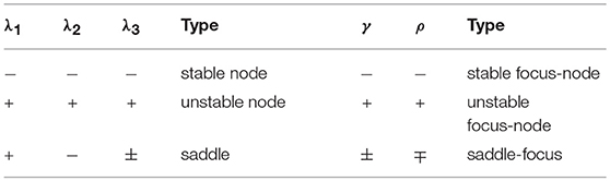
Table 1. Behavior of 3D-systems near hyperbolic equilibrium points with Jacobi matrix having either three real eigenvalues λ_i or two complex eigenvalues λ_2/3 = ρ±iω and a real eigenvalue λ₁ = γ.

FIGURE 1

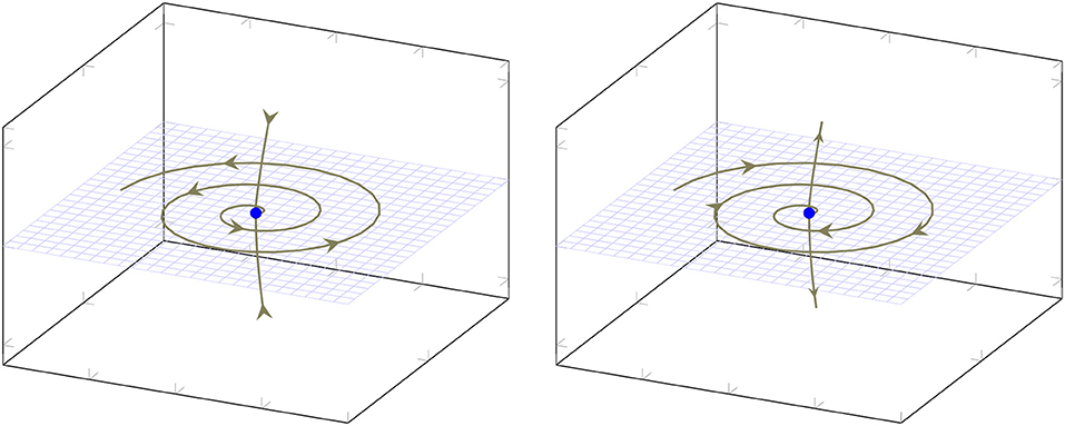
Figure 1. Two types of saddle-foci: On the left the two-dimensional eigenmanifold is unstable and the one-dimensional eigenmanifold is stable, while on the right it is vice versa.

2.3. Data

The investigated data consists of ten EEG data sets of epileptic patients suffering from petit mal (absence) seizures. To avoid a biased investigation two different sources of data sets were investigated.

The first source contains eight different EEG data sets from two different patients kindly provided by the Epilepsy Centre at the Department of Neurology Erlangen. The data was sampled from 25 electrodes using the modified 10/20 system with 10% electrode positions and modified combinatorial nomenclature. The length of the data sets vary between 5 and 10 min each sampled with a sample rate of 256 Hz. Each data set contains at least one absence seizure with a length of about 4 up to 16 s.

The second source is the Temple University Hospital EEG Data Corpus [19] again sampled using the 10/20 system in this case with a sample rate of 250 Hz, length of datasets 24 and 20 min, each with absence seizures of between 19 and 144 s.

As preprocessing step we applied a zerophase bandpass filter with cut-off frequencies 0.5 and 30 Hz. From the above mentioned data sets we investigated 10 signals of 20–40 s length and partitioned the data into parts of 2 s length with an rectangular window, as we want the time-domain of the signal to be preserved. This resulted in a total of 129 investigated windows of EEG signal.

3. Results

To illustrate the application of DSBM, Figure 2 presents the obtained minimal values of the cost function (7) applied to a two-second-windowed data set. The backround plot represents the signal of the F4 electrode. The sequence of the minimal values show that the model assumption Equation (10) fits well to describe the time evolution during a petit mal seizure. As is shown in Figure 3 in most cases the representation of the ictal dynamics using Equation (10) is above 90%.

FIGURE 2

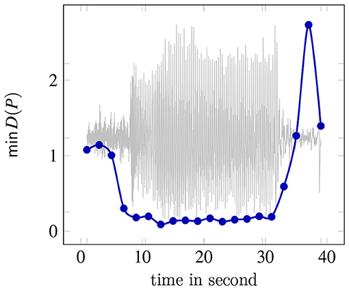
Figure 2. Minmal values of the cost function of DSBM (7) on a two-second-windowed data set. In the background the signal of the F4 electrode is shown.

FIGURE 3

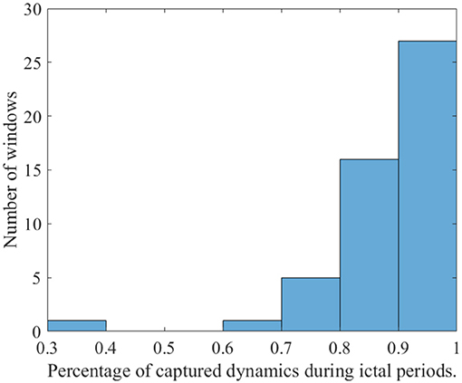
Figure 3. Histogram of the signal representation during ictal periods.

To evaluate the significance of the minimal D(P)-value drop during seizures, thresholds based on leave-one-out cross-validation are trained to separate ictal from interictal phases. This validation yields a specifity of 84% and a sensitivity of 75% with respect to the appearance of spike-waves averaged over all 129 windowed data.

As described in section 2 the minimum of D(P) corresponds to an optimal projection P with respect to the underlying model dynamics. Applying the projection P onto the 25-dimensional signal q(t) three amplitudes x_i(t) are obtained: (Pq)_i = x_i(t), i = 1, 2, 3. Thereby the 25-dimensional original phase space trajectory is now projected onto a three-dimensional phase portrait given by the amplitudes x₁(t), x₂(t), and x₃(t). Figure 4 shows on the right-hand side a typical trajectory. For the same time window a decomposition via PCA and ICA were performed and the corresponding phase portraits are shown on the left and the middle. In the case of PCA the first three vectors representing most of the signal are utilized for the projection. For ICA three projection vectors are chosen leading to the best structured phase portrait. The advantage of DSBM compared to PCA or ICA is obvious. A clear structure can only be detected in the case of the trajectories obtained by DSBM.

FIGURE 4

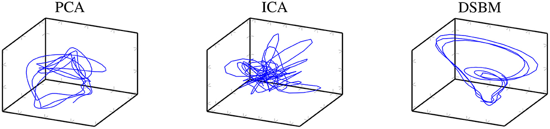
Figure 4. Phase portraits of amplitudes obtained by PCA (first three dominant amplitudes), ICA (three amplitudes with best structured phase portrait) and DSBM.

Figure 5 shows the vectors of the pseudoinverse P⁺ caculated from eq. (8). By this projection method the original signal q(t) is filtered to $q_f(t)=P^{+}Pq(t)$.

FIGURE 5

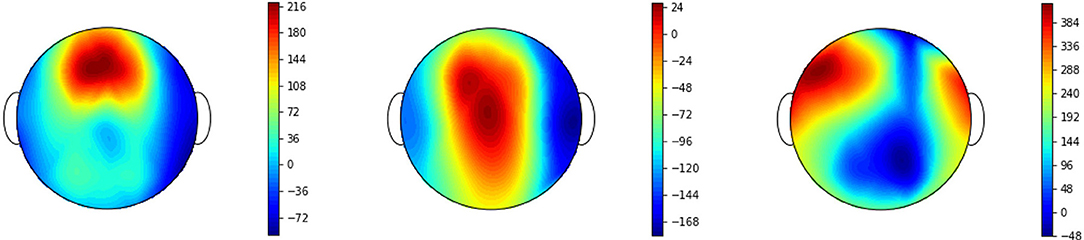
Figure 5. Potential field maps representing the vectors of the calculated pseudoinverse.

Figure 6 shows the original signal of one electrode of an exemplary absence signal and the corresponding approximation. The main structure of the signal is captured. I.e., we are dealing with a projection fulfilling our model equations (10) and representing the signal to a considerable amount.

FIGURE 6

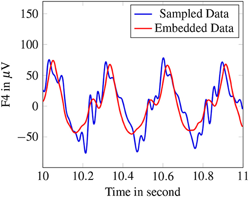
Figure 6. Original signal of F4-electrode compared to reconstructed signal after embedding with the pseudoinverse.

The final step of our investigation aimed at characterizing and comparing the projected signal dynamics of the windowed EEG data epochs representing a good fit of the model, i.e., possessing a low minimal cost function value D(P) = 0.3, i.e., dynamics representation of above 90%.

To achieve this, for each optimal projection the set of obtained differential equations was investigated with respect to occuring equilibrium points and linear stabilty analysis. For 70% of all investigated data epochs, the Shilnikov condition was fulfilled.

In addition, visual inspections of the phase portraits were performed to quantify the occurrence of a Shilnikov type of homoclinic orbit. Figure 7 shows two examples of the projected signals. The phase portrait on the left hand side seems to represent a homoclinic orbit near the equilibrium point, whereas the trajectory on the right hand side resembles more a circle and not a homoclinic orbit based at the equilibrium point.

FIGURE 7

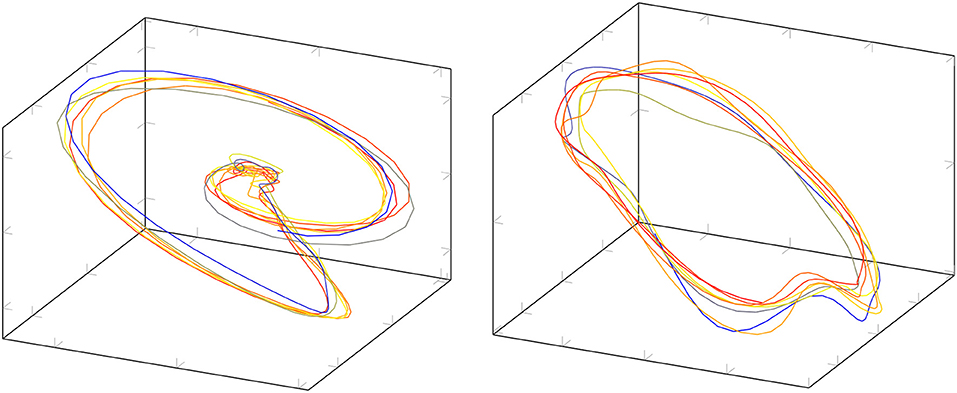
Figure 7. Examples of the projected signal in phase space. The example on the left hand side seems to represent a homoclinic orbit, the trajectory on the right hand resembles a circle. The color indicates the time evolution of the trajectory.

Accounting these visual inspections, we obtained the fourfold table presented in Table 2.

TABLE 2

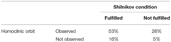
Table 2. Four-fold table evalutating Shilnikov condition and homoclinic orbit in data epochs well-described by the assumed model.

4. Discussion

If one is interested in representing a high-dimensional multivariate signal as a trajectory in a low-dimensional phase space, DSBM is an adequate tool. This is illustrated in our investigation of EEG data of epileptic seizure by Figure 4 showing a clearly better structure of the trajectory compared to signal decomposition techniques like PCA, ICA, and all other techniques we investigated. This is due to the different approaches: PCA, ICA, and other techniques (see, e.g., [20]) are based on stochastic model assumptions, whereas DSBM intends to represent the signal in terms of the underlying dynamic interactions. These dynamic interactions are incorporated in DSBM by a model of a set of differential equations with its parameters being approximated simultaneously with the parameters of the best fitting projections.

We showed that the assumption of a special set of differential equations (10) fits well to the occurrence of seizures by a dramatic drop of the optimized cost function. Although not intending to develop an algorithm for seizure detection we calculated the specifity and sensitivity of DSBM with respect to ictal and interictal phases of the signal and could confirm the correlation of cost function drop with the occurence of absence seizures to an extent of 80%.

The obtained trajectories in phase space resemble the chaotic behavior of Shilnikov dynamics. The investigation in a moving window setup showed that the approximated dynamics fulfil the Shilnikov condition in 69% of all ictal signal windows. However not all of these dynamics show a homoclinic orbit by visual inspection. This is in accordance to the microscopic model investigated in van Veen and Liley [4], where both chaotic bahavior due to the Shilnikov setting and periodic solutions are observed.

Limitations of our approach are (i) possible non-stationarities of the signal, (ii) a not optimal choice of set of ODEs as the underlying model, (iii) sensitivity of the non-linear ODEs with respect to occuring fixed points and therefore instabilities by comparing the parameter space of the ODEs and/or (iv) instabilities in the global optimization procedure of the cost function.

Even though the stability analysis did not completely confirm the appearance of Shilnikov chaos in EEG data, it was shown that the mathematical theorems are applicaple in data-driven situations. The study reveals that one can validate Shilnikov chaos in EEG signals on a data-driven basis and one is not ought to tweak a set of differential equations by hand to do so.

Further work will focus on the development of projection algorithms independent of choosing a set of ODEs obtained by solving a generalized eigenvalue problem as presented in Seifert et al. [21].

Ethics Statement

The investigated data was taken partly from the previously published data set [19] and partly from data collected for medical reasons. The data obtained is completely anonymized. Hence by local legislation no approval by an ethics committe is required.

Author Contributions

BS contributed to the data analysis and the manuscript. DA contributed to the data analysis. CU conceived the structure of the study and contributed to the manuscript.

Conflict of Interest Statement

The authors declare that the research was conducted in the absence of any commercial or financial relationships that could be construed as a potential conflict of interest.

Acknowledgments

We acknowledge funding by the European Regional Development Fund (ERDF) and the support by the Bayerische Forschungsstiftung within the project Nilpherd. We thank the Epilepsy Centre at the Department of Neurology, Universitätsklinikum Erlangen for provided data and BESA GmbH and Epilepsy Centre for fruitful ideas and discussions.

References

1. Pearson K. On lines and planes of closest fit to a system of points in space. Lond Edinburgh Dublin Philos Mag J Sci. (1901) 6:559–72.

Google Scholar

2. Hyvärinen A, Oja E. Independent component analysis: algorithms and applications. Neural Netw. (2000) 13:411–30. doi: 10.1016/S0893-6080(00)00026-5

PubMed Abstract | CrossRef Full Text | Google Scholar

3. Uhl C, Seifert B. DSBM - dynamical systems based modeling: an overview. In: Ambrosius U, Gollisch S, editors. Ansbacher Kaleidoskop 2016. Shaker Verlag (2016). p. 123–38.

Google Scholar

4. van Veen L, Liley DTJ. Chaos via Shilnikov's Saddle-Node bifurcation in a theory of the electroencephalogram. Phys Rev Lett. (2006) 97:208101. doi: 10.1103/PhysRevLett.97.208101

CrossRef Full Text | Google Scholar

5. Friedrich R, Haken H. Time-dependent and chaotic behaviour in systems with O(3)-symmetry. In: Güttinger W, Dangelmayer G, editors. The Physics of Structure Formation: Theory and Simulation. Springer (1987). p. 334–45.

Google Scholar

6. Friedrich R, Uhl C. Spatio-temporal analysis of human electroencephalograms: petit-mal epilepsy. Phys D (1996) 98:171–82. doi: 10.1016/0167-2789(96)00059-0

CrossRef Full Text | Google Scholar

7. Uhl C. Analyse raumzeitlicher Daten strukturbildender Systeme. Universität Stuttgart (1995).

8. Kabir E, Siuly Zhang Y. Epileptic seizure detection from EEG signals using logistic model trees. Brain Inform. (2016) 3:93–100. doi: 10.1007/s40708-015-0030-2

PubMed Abstract | CrossRef Full Text | Google Scholar

9. Lehnertz K, Andrzejak R, Arnhold J, Kreuz T, Mormann F, Rieke C, et al. Nonlinear EEG analysis in epilepsy: its possible use for interictal focus localization, seizure anticipation, and prevention. J Clin Neurophysiol. (2001) 18:209–22.

PubMed Abstract | Google Scholar

10. Aschenbrenner-Scheibe R, Maiwald T, Winterhalder M, Voss HU, Timmer J, Schulze-Bonhage A. How well can epileptic seizures be predicted? An evaluation of a nonlinear method. Brain (2003) 126:2616–26. doi: 10.1093/brain/awg265

PubMed Abstract | CrossRef Full Text | Google Scholar

11. Uhl C, Kruggel F, Opitz B, von Cramon DY. A new concept for EEG/MEG signal analysis: detection of interacting spatial modes. Human Brain Mapp. (1998) 6:137–49. doi: 10.1002/(SICI)1097-0193(1998)6:3<137::AID-HBM3>3.0.CO;2-4

PubMed Abstract | CrossRef Full Text | Google Scholar

12. Hüper K, Trumpf J. Newton-like methods for numerical optimisation on manifolds. In: Proceedings of the Thirty-Eighth Asilomar Conference on Signals, Systems and Computers. Monterey, CA (2004). p. 136–9. doi: 10.1109/ACSSC.2004.1399106

CrossRef Full Text | Google Scholar

13. Helmke U, Moore JB. Optimization and Dynamical Systems. London: Springer-Verlag (1994).

14. More JJ. Levenberg–Marquardt algorithm: implementation and theory. In: Watson GA, editor. Numerical Analysis. Springer (1977). p. 105–16. Available online at: http://www.osti.gov/scitech/servlets/purl/7256021.

Google Scholar

15. Hutt A, Svensén M, Kruggel F, Friedrich R. Detection of fixed points in spatiotemporal signals by a clustering method. Phys Rev E. (2000) 61:R4691–3. doi: 10.1103/PhysRevE.61.R4691

PubMed Abstract | CrossRef Full Text | Google Scholar

16. Hartman P. A Lemma in the theory of structural stability of differential equations. Proc Am Math Soc. (1960) 11:610–20. doi: 10.1090/S0002-9939-1960-0121542-7

CrossRef Full Text | Google Scholar

17. Shilnikov LP. A case of the existence of a denumerable set of periodic motions. Sov Math Dokl. (1965) 6:163–6.

Google Scholar

18. Arneodo A, Coullet P, Tresser C. Possible new strange attractors with spiral structure. Commun Math Phys. (1981) 79:573–9.

Google Scholar

19. Obeid I, Picone J. The Temple University Hospital EEG data corpus. Front Neurosci. (2016) 10:196. doi: 10.3389/fnins.2016.00196

PubMed Abstract | CrossRef Full Text | Google Scholar

20. Pena D, Poncela P. Dimension reduction in multivariate time series. In: Balakrishnan N, Sarabia JM, Castillo E, editors. Advances in Distribution Theory, Order Statistics, and Inference. Springer (2006). p. 433–58.

Google Scholar

21. Seifert B, Korn K, Hartmann S, Uhl C. Dynamical Component Analysis (DyCA): Dimensionality reduction for high-dimensional deterministic time-series. In: 2018 IEEE 28th International Workshop on Machine Learning for Signal Processing (MLSP) (Aalborg) (2018).

Google Scholar