Randomized Distributed Mean Estimation: Accuracy vs. Communication

1. Introduction

We address the problem of estimating the arithmetic mean of n vectors, $X_1,\dots ,X_n\in {ℝ}^d$, stored in a distributed fashion across n compute nodes, subject to a constraint on the communication cost.

In particular, we consider a star network topology with a single server at the centre and n nodes connected to it. All nodes send an encoded (possibly via a lossy randomized transformation) version of their vector to the server, after which the server performs a decoding operation to estimate the true mean

$X\stackrel{\text{def}}{=}\frac{1}{n}{\displaystyle \sum _{i=1}^n{X}_i}.$

The purpose of the encoding operation is to compress the vector so as to save on communication cost, which is typically the bottleneck in practical applications.

To better illustrate the setup, consider the naive approach in which all nodes send the vectors without performing any encoding operation, followed by the application of a simple averaging decoder by the server. This results in zero estimation error at the expense of maximum communication cost of ndr bits, where r is the number of bits needed to communicate a single floating point entry/coordinate of X_i.

This operation appears as a computational primitive in numerous cases, and the communication cost can be reduced at the expense of acurracy. Our proposal for balancing accuracy and communication is in practice relevant for any application that uses the MPI_Gather or MPI_Allgather routines [1], or their conceptual variants, for efficient implementation and can tolerate inexactness in compuation, such as many algorithms for distributed optimization.

1.1. Background and Contributions

The distributed mean estimation problem was recently studied in a statistical framework where it is assumed that the vectors X_i are independent and identicaly distributed samples from some specific underlying distribution. In such a setup, the goal is to estimate the true mean of the underlying distribution [2–5]. These works formulate lower and upper bounds on the communication cost needed to achieve the minimax optimal estimation error.

In contrast, we do not make any statistical assumptions on the source of the vectors, and study the trade-off between expected communication costs and mean square error of the estimate. Arguably, this setup is a more robust and accurate model of the distributed mean estimation problems arising as subproblems in applications such as reduce-all operations within algorithms for distributed and federated optimization [6–10]. In these applications, the averaging operations need to be done repeatedly throughout the iterations of a master learning/optimization algorithm, and the vectors {X_i} correspond to updates to a global model/variable. In such cases, the vectors evolve throughout the iterative process in a complicated pattern, typically approaching zero as the master algorithm converges to optimality. Hence, their statistical properties change, which renders fixed statistical assumptions not satisfied in practice.

For instance, when training a deep neural network model in a distributed environment, the vector X_i corresponds to a stochastic gradient based on a minibatch of data stored on node i. In this setup we do not have any useful prior statistical knowledge about the high-dimensional vectors to be aggregated. It has recently been observed that when communication cost is high, which is typically the case for commodity clusters, and even more so in a federated optimization framework, it is can be very useful to sacrifice on estimation accuracy in favor of reduced communication [11, 12].

In this paper we propose a parametric family of randomized methods for estimating the mean X, with parameters being a set of probabilities p_ij for i = 1, …, n and j = 1, 2, …, d and node centers μ_i ∈ ℝ for i = 1, 2, …, n. The exact meaning of these parameters is explained in section 3. By varying the probabilities, at one extreme, we recover the exact method described, enjoying zero estimation error at the expense of full communication cost. At the opposite extreme are methods with arbitrarily small expected communication cost, which is achieved at the expense of suffering an exploding estimation error. Practical methods appear somewhere on the continuum between these two extremes, depending on the specific requirements of the application at hand. Suresh et al. [13] propose a method combining a pre-processing step via a random structured rotation, followed by randomized binary quantization. Their quantization protocol arises as a suboptimal special case of our parametric family of methods¹.

To illustrate our results, consider the special case presented in Example 7, in which we choose to communicate a single bit per element of X_i only. We then obtain an ${O}(\frac{r}{n}R)$ bound on the mean square error, where r is number of bits used to represent a floating point value, and $R=\frac{1}{n}\sum _{i=1}^n\Vert X_i-{\mu }_{i}1{\Vert }^2$ with μ_i ∈ ℝ being the average of elements of X_i, and 1 the all-ones vector in ℝ^d. Note that this bound improves upon the performance of the method of Suresh et al. [13] in two aspects. First, the bound is independent of d, improving from logarithmic dependence, as stated in Remark 4 in detail. Further, due to a preprocessing rotation step, their method requires ${O}(dlogd)$ time to be implemented on each node, while our method is linear in d. This and other special cases are summarized in Table 1 in section 5.

TABLE 1

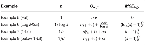
Table 1. Summary of achievable communication cost and estimation error, for various choices of probability p.

While the above already improves upon the state of the art, the improved results are in fact obtained for a suboptimal choice of the parameters of our method (constant probabilities p_ij, and node centers fixed to the mean μ_i). One can decrease the MSE further by optimizing over the probabilities and/or node centers (see section 6). However, apart from a very low communication cost regime in which we have a closed form expression for the optimal probabilities, the problem needs to be solved numerically, and hence we do not have expressions for how much improvement is possible. We illustrate the effect of fixed and optimal probabilities on the trade-off between communication cost and MSE experimentally on a few selected datasets in section 6 (see Figure 1).

FIGURE 1

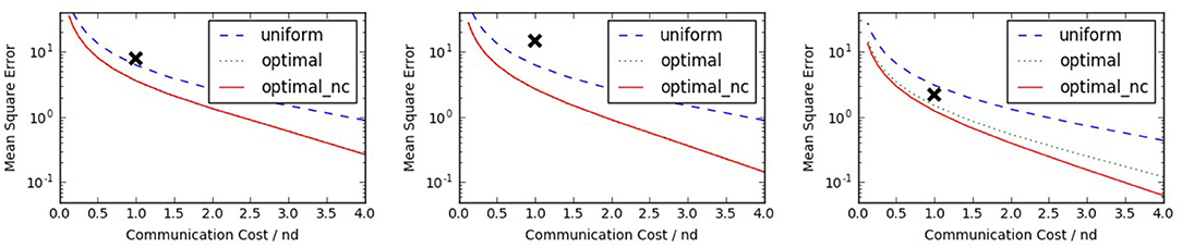
Figure 1. Trade-off curves between communication cost and estimation error (MSE) for four protocols. The plots correspond to vectors X_i drawn in an i.i.d. fashion from Gaussian, Laplace, and χ² distributions, from left to right. The black cross marks the performance of binary quantization (Example 4).

Remark 1. Since the initial version of this work, an updated version of Suresh et al. [13] contains a rate similar to Example 7, using variable length coding. That work also formulates lower bounds, which are attained by both their and our results. Other works that were published since, such as [14, 15], propose algorithms that can also be represented as a particular choice of protocols α, β, γ, demonstrating the versatility of our proposal.

1.2. Outline

In section 2 we formalize the concepts of encoding and decoding protocols. In section 3 we describe a parametric family of randomized (and unbiased) encoding protocols and give a simple formula for the mean squared error. Subsequently, in section 4 we formalize the notion of communication cost, and describe several communication protocols, which are optimal under different circumstances. We give simple instantiations of our protocol in section 5, illustrating the trade-off between communication costs and accuracy. In section 6 we address the question of the optimal choice of parameters of our protocol. Finally, in section 7 we comment on possible extensions we leave out to future work.

2. Three Protocols

In this work we consider (randomized) encoding protocols α, communication protocols β, and decoding protocols γ using which the averaging is performed inexactly as follows. Node i computes a (possibly stochastic) estimate of X_i using the encoding protocol, which we denote $Y_i=\alpha (X_i)\in {ℝ}^d$, and sends it to the server using communication protocol β. By β(Y_i) we denote the number of bits that need to be transferred under β. The server then estimates X using the decoding protocol γ of the estimates:

$Y\stackrel{\text{def}}{=}\gamma \left(Y_1,\dots ,Y_n\right).$

The objective of this work is to study the trade-off between the (expected) number of bits that need to be communicated, and the accuracy of Y as an estimate of X.

In this work we focus on encoders which are unbiased, in the following sense.

Definition 2.1 (Unbiased and Independent Encoder): We say that encoder α is unbiased if E_α[α(X_i)] = X_i for all i = 1, 2, …, n. We say that it is independent, if α(X_i) is independent from α(X_j) for all i ≠ j.

Example 1 (Identity Encoder). A trivial example of an encoding protocol is the identity function: α(X_i) = X_i. It is both unbiased and independent. This encoder does not lead to any savings in communication that would be otherwise infeasible though.

Another examples of unbiased and independent Encoders include the protocols introduced in section 3, or other existing techniques [12, 14, 15].

We now formalize the notion of accuracy of estimating X via Y. Since Y can be random, the notion of accuracy will naturally be probabilistic.

Definition 2.2 (Estimation Error / Mean Squared Error): The mean squared error of protocol (α, γ) is the quantity

$\begin{array}{l}MS{E}_{\alpha ,\gamma }\left(X_1,\dots ,X_n\right)=E_{\alpha ,\gamma }\left[\Vert Y-X{\Vert }^2\right]\\ =E_{\alpha ,\gamma }{\left[\Vert \gamma (\alpha (X_1),\dots ,\alpha (X_n))-X\Vert \right]}^2.\end{array}$

To illustrate the above concept, we now give a few examples:

Example 2 (Averaging Decoder). If γ is the averaging function, i.e., $\gamma (Y_1,\dots ,Y_n)=\frac{1}{n}{\sum }_{i=1}^n{Y}_i,$ then

$MS{E}_{\alpha ,\gamma }(X_1,\dots ,X_n)=\frac{1}{n^2}{E}_{\alpha }\left[{\Vert {\displaystyle \sum _{i=1}^n\left(\alpha (X_i)-X_i\right)}\Vert }^2\right].$

The next example generalizes the identity encoder and averaging decoder.

Example 3 (Linear Encoder and Inverse Linear Decoder). Let A:ℝ^d → ℝ^d be linear and invertible. Then we can set $Y_i=\alpha (X_i)\stackrel{\mathrm{\text{def}}}{=}A{X}_i$ and $\gamma (Y_1,\dots ,Y_n)\stackrel{\mathrm{\text{def}}}{=}{A}^{-1}(\frac{1}{n}{\sum }_{i=1}^n{Y}_i)$. If A is random, then α and γ are random (e.g., a structured random rotation, see [16]). Note that

$\gamma \left(Y_1,\dots ,Y_n\right)=\frac{1}{n}{\displaystyle \sum _{i=1}^n{A}^{-1}}{Y}_i=\frac{1}{n}{\displaystyle \sum _{i=1}^n{X}_i}=X,$

and hence the MSE of (α, γ) is zero.

We shall now prove a simple result for unbiased and independent encoders used in subsequent sections.

Lemma 2.3 (Unbiased and Independent Encoder + Averaging Decoder): If the encoder α is unbiased and independent, and γ is the averaging decoder, then

$\begin{array}{l}MS{E}_{\alpha ,\gamma }\left(X_1,\dots ,X_n\right)=\frac{1}{n^2}{\displaystyle \sum _{i=1}^n{E}_{\alpha }}\left[\Vert Y_i-X_i{\Vert }^2\right]\\ =\frac{1}{n^2}{\displaystyle \sum _{i=1}^{n}Va{r}_{\alpha }}\left[\alpha (X_i)\right].\end{array}$

Proof. Note that E_α[Y_i] = X_i for all i. We have

$\begin{array}{l}MS{E}_{\alpha }\left(X_1,\dots ,X_n\right)=E_{\alpha }\left[\Vert Y-X{\Vert }^2\right]\\ =\frac{1}{n^2}{E}_{\alpha }\left[{\Vert {\displaystyle \sum _{i=1}^n{Y}_i}-X_i\Vert }^2\right]\\ \stackrel{(*)}{=}\frac{1}{n^2}{\displaystyle \sum _{i=1}^n{E}_{\alpha }}\left[{\Vert Y_i-E_{\alpha }\left[Y_i\right]\Vert }^2\right]\\ =\frac{1}{n^2}{\displaystyle \sum _{i=1}^{n}Va{r}_{\alpha }}\left[\alpha (X_i)\right],\end{array}$

where (*) follows from unbiasedness and independence.      □

One may wish to define the encoder as a combination of two or more separate encoders: α(X_i) = α₂(α₁(X_i)). See Suresh et al. [13] for an example where α₁ is a random rotation and α₂ is binary quantization.

3. A Family of Randomized Encoding Protocols

Let $X_1,\dots ,X_n\in {ℝ}^d$ be given. We shall write X_i = (X_i(1), …, X_i(d)) to denote the entries of vector X_i. In addition, with each i we also associate a parameter μ_i ∈ ℝ. We refer to μ_i as the center of data at node i, or simply as node center. For now, we assume these parameters are fixed. As a special case, we recover for instance classical binary quantization, see section 5.1. We shall comment on how to choose the parameters optimally in section 6.

We shall define support of α on node i to be the set $S_i\stackrel{\mathrm{\text{def}}}{=}\left\{j:Y_i(j)\ne {\mu }_i\right\}$. We now define two parametric families of randomized encoding protocols. The first results in S_i of random size, the second has S_i of a fixed size.

3.1. Encoding Protocol With Variable-Size Support

With each pair (i, j) we associate a parameter 0 < p_ij ≤ 1, representing a probability. The collection of parameters {p_ij, μ_i} defines an encoding protocol α as follows:

$\begin{array}{ll}{Y}_i\left(j\right)=\{\begin{array}{ll}\frac{X_i(j)}{p_{ij}}-\frac{1-p_{ij}}{p_{ij}}{\mu }_i\hfill & \text{ with probability }{p}_{ij},\hfill \\ {\mu }_i\hfill & \text{ with probability }1-p_{ij}.\hfill \end{array}& (1)\end{array}$

Remark 2. Enforcing the probabilities to be positive, as opposed to non-negative, leads to vastly simplified notation in what follows. However, it is more natural to allow p_ij to be zero, in which case we have Y_i(j) = μ_i with probability 1. This raises issues such as potential lack of unbiasedness, which can be resolved, but only at the expense of a larger-than-reasonable notational overload.

In the rest of this section, let γ be the averaging decoder (Example 2). Since γ is fixed and deterministic, we shall for simplicity write E_α[·] instead of E_{α, γ}[·]. Similarly, we shall write MSE_α(·) instead of MSE_{α, γ}(·).

We now prove two lemmas describing properties of the encoding protocol α. Lemma 3.1 states that the protocol yields an unbiased estimate of the average X and Lemma 3.2 provides the expected mean square error of the estimate.

Lemma 3.1 (Unbiasedness): The encoder α defined in (1) is unbiased. That is, E_α[α(X_i)] = X_i for all i. As a result, Y is an unbiased estimate of the true average: E_α[Y] = X.

Proof. Due to linearity of expectation, it is enough to show that E_α[Y(j)] = X(j) for all j. Since $Y(j)=\frac{1}{n}{\sum }_{i=1}^n{Y}_i(j)$ and $X(j)=\frac{1}{n}{\sum }_{i=1}^n{X}_i(j)$, it suffices to show that E_α[Y_i(j)] = X_i(j):

$E_{\alpha }\left[Y_i(j)\right]=p_{ij}\left(\frac{X_i(j)}{p_{ij}}-\frac{1-p_{ij}}{p_{ij}}{\mu }_i(j)\right)+(1-p_{ij}){\mu }_i(j)=X_i(j),$

and the claim is proved.       □

Lemma 3.2 (Mean Squared Error): Let α = α(p_ij, μ_i) be the encoder defined in (1). Then

$\begin{array}{ll}MS{E}_{\alpha }(X_1,\dots ,X_n)=\frac{1}{n^2}{\displaystyle \sum _{i,j}\left(\frac{1}{p_{ij}}-1\right)}{\left(X_i(j)-{\mu }_i\right)}^2.& (2)\end{array}$

Proof. Using Lemma 3.2, we have

$\begin{array}{l}MS{E}_{\alpha }(X_1,\dots ,X_n)=\frac{1}{n^2}{\displaystyle \sum _{i=1}^n{E}_{\alpha }}\left[{\Vert Y_i-X_i\Vert }^2\right]\\ =\frac{1}{n^2}{\displaystyle \sum _{i=1}^n{E}_{\alpha }}\left[{\displaystyle \sum _{j=1}^d(Y_i(}j)-X_i(j){)}^2\right]\\ =\frac{1}{n^2}{\displaystyle \sum _{i=1}^n{\displaystyle \sum _{j=1}^d{E}_{\alpha }}}\left[{(Y_i(j)-X_i(j))}^2\right].& (3)\end{array}$

For any i, j we further have

$\begin{array}{l}{E}_{\alpha }\left[{(Y_i(j)-X_i(j))}^2\right]=p_{ij}{\left(\frac{X_i(j)}{p_{ij}}-\frac{1-p_{ij}}{p_{ij}}{\mu }_i-X_i(j)\right)}^2\\ +(1-p_{ij}){\left({\mu }_i-X_i(j)\right)}^2\\ =\frac{{(1-p_{ij})}^2}{p_{ij}}{\left(X_i(j)-{\mu }_i\right)}^2\\ +(1-p_{ij}){\left({\mu }_i-X_i(j)\right)}^2\\ =\left(\frac{1-p_{ij}}{p_{ij}}\right){\left(X_i(j)-{\mu }_i\right)}^2.\end{array}$

It suffices to substitute the above into (3).       □

3.2. Encoding Protocol With Fixed-Size Support

Here we propose an alternative encoding protocol, one with deterministic support size. As we shall see later, this results in deterministic communication cost.

Let σ_k(d) denote the set of all subsets of {1, 2, …, d} containing k elements. The protocol α with a single integer parameter k is then working as follows: First, each node i samples ${{D}}_i\in {\sigma }_k(d)$ uniformly at random, and then sets

$\begin{array}{ll}{Y}_i(j)=\{\begin{array}{ll}\frac{d{X}_i(j)}{k}-\frac{d-k}{k}{\mu }_i\hfill & \text{ if }j\in {\mathcal{D}}_i,\hfill \\ {\mu }_i\hfill & \text{ otherwise}.\hfill \end{array}& (4)\end{array}$

Note that due to the design, the size of the support of Y_i is always k, i.e., |S_i| = k. Naturally, we can expect this protocol to perform practically the same as the protocol (1) with p_ij = k/d, for all i, j. Lemma 3.4 indeed suggests this is the case. While this protocol admits a more efficient communication protocol (as we shall see in section 4.4), protocol (1) enjoys a larger parameters space, ultimately leading to better MSE. We comment on this tradeoff in subsequent sections.

As for the data-dependent protocol, we prove basic properties. The proofs are similar to those of Lemmas 3.1 and 3.2 and we defer them to Appendix A.

Lemma 3.3 (Unbiasedness): The encoder α defined in (4) is unbiased. That is, E_α[α(X_i)] = X_i for all i. As a result, Y is an unbiased estimate of the true average: E_α[Y] = X.

Lemma 3.4 (Mean Squared Error): Let α = α(k) be encoder defined as in (4). Then

$\begin{array}{ll}MS{E}_{\alpha }(X_1,\dots ,X_n)=\frac{1}{n^2}{\displaystyle \sum _{i=1}^n{\displaystyle \sum _{j=1}^d\left(\frac{d-k}{k}\right)}}{\left(X_i(j)-{\mu }_i\right)}^2.& (5)\end{array}$

4. Communication Protocols

Having defined the encoding protocols α, we need to specify the way the encoded vectors Y_i = α(X_i), for i = 1, 2, …, n, are communicated to the server. Given a specific communication protocol β, we write β(Y_i) to denote the (expected) number of bits that are communicated by node i to the server. Since Y_i = α(X_i) is in general not deterministic, β(Y_i) can be a random variable.

Definition 4.1 (Communication Cost): The communication cost of communication protocol β under randomized encoding α is the total expected number of bits transmitted to the server:

$\begin{array}{ll}{C}_{\alpha ,\beta }(X_1,\dots ,X_n)=E_{\alpha }\left[{\displaystyle \sum _{i=1}^n\beta }(\alpha (X_i))\right].& (6)\end{array}$

Given Y_i, a good communication protocol is able to encode Y_i = α(X_i) using a few bits only. Let r denote the number of bits used to represent a floating point number. Let $\bar{r}$ be the the number of bits representing μ_i.

In the rest of this section we describe several communication protocols β and calculate their communication cost.

4.1. Naive

Represent Y_i = α(X_i) as d floating point numbers. Then for all encoding protocols α and all i we have β(α(X_i)) = dr, whence

$C_{\alpha ,\beta }=E_{\alpha }\left[{\displaystyle \sum _{i=1}^n\beta }(\alpha (X_i))\right]=ndr.$

4.2. Varying-Length

We will use a single variable for every element of the vector Y_i, which does not have constant size. The first bit decides whether the value represents μ_i or not. If yes, end of variable, if not, next r bits represent the value of Y_i(j). In addition, we need to communicate μ_i, which takes $\bar{r}$ bits². We thus have

$\begin{array}{ll}\beta (\alpha (X_i))=\overline{r}+{\displaystyle \sum _{j=1}^d\left(1_{(Y_i(j)={\mu }_i)}+(r+1)\times 1_{(Y_i(j)\ne {\mu }_i)}\right)},& (7)\end{array}$

where 1_e is the indicator function of event e. The expected number of bits communicated is given by

$\begin{array}{l}{C}_{\alpha ,\beta }=E_{\alpha }\left[{\displaystyle \sum _{i=1}^n\beta }(\alpha (X_i))\right]\stackrel{\left(7\right)}{=}n\overline{r}+{\displaystyle \sum _{i=1}^n{\displaystyle \sum _{j=1}^d\left(1-p_{ij}+(r+1)p_{ij}\right)}}\\ =n\overline{r}+{\displaystyle \sum _{i=1}^n{\displaystyle \sum _{j=1}^d\left(1+r{p}_{ij}\right)}}\end{array}$

In the special case when p_ij = p > 0 for all i, j, we get

$C_{\alpha ,\beta }=n(\overline{r}+d+pdr).$

4.3. Sparse Communication Protocol for Encoder (1)

We can represent Y_i as a sparse vector; that is, a list of pairs (j, Y_i(j)) for which Y_i(j) ≠ μ_i. The number of bits to represent each pair is ⌈log(d)⌉ + r. Any index not found in the list, will be interpreted by server as having value μ_i. Additionally, we have to communicate the value of μ_i to the server, which takes $\bar{r}$ bits. We assume that the value d, size of the vectors, is known to the server. Hence,

$\beta (\alpha (X_i))=\overline{r}+{\displaystyle \sum _{j=1}^d{1}_{(Y_i(j)\ne {\mu }_i)}}\times \left(\lceil \text{log }d\rceil +r\right).$

Summing up through i and taking expectations, the the communication cost is given by

$\begin{array}{ll}{C}_{\alpha ,\beta }=E_{\alpha }\left[{\displaystyle \sum _{i=1}^n\beta }(\alpha (X_i))\right]=n\overline{r}+(\lceil \text{log }d\rceil +r){\displaystyle \sum _{i=1}^n{\displaystyle \sum _{j=1}^d{p}_{ij}}}.& (8)\end{array}$

In the special case when p_ij = p > 0 for all i, j, we get

$C_{\alpha ,\beta }=n\overline{r}+(\lceil \text{log }d\rceil +r)ndp.$

Remark 3. A practical improvement upon this could be to (without loss of generality) assume that the pairs (j, Y_i(j)) are ordered by j, i.e., we have ${\left\{(j_s,Y_i(j_s))\right\}}_{s=1}^k$ for some k and j₁ < j₂ < ⋯ < j_k. Further, let us denote j₀ = 0. We can then use a variant of variable-length quantity [17] to represent the set ${\left\{(j_s-j_{s-1},Y_i(j_s))\right\}}_{s=1}^k$. With careful design one can hope to reduce the log(d) factor in the average case. Nevertheless, this does not improve the worst case analysis we focus on in this paper, and hence we do not delve deeper in this. After the first version of this work was posted on arXiv, such an idea was independently proposed and analyzed in Alistarh et al. [14].

4.4. Sparse Communication Protocol for Encoder (4)

We now describe a sparse communication protocol compatible with fixed length encoder defined in (4). Note that the selection of set ${{D}}_i$ is independent of the values X_i(j) being compressed. We can utilize this fact, and instead of communicating index-value pairs (j, Y_i(j)) as above, we can only communicate the values Y_i(j), and the indices they correspond to can be reconstructed from a shared random seed. This lets us avoid the log(d) factor in (8). Apart from protocol (4), this idea is also applicable to protocol (1) with uniform probabilities p_ij.

In particular, we represent Y_i as a vector containing the list of the values for which Y_i(j) ≠ μ_i, ordered by j. Additionally, we communicate the value μ_i (using $\bar{r}$ bits) and a random seed (using ${\bar{r}}_s$ bits), which can be used to reconstruct the indices j, corresponding to the communicated values. Note that for any fixed k defining protocol (4), we have |S_i| = k. Hence, communication cost is deterministic:

$\begin{array}{ll}{C}_{\alpha ,\beta }={\displaystyle \sum _{i=1}^n\beta }(\alpha (X_i))=n(\overline{r}+{\overline{r}}_s)+nkr.& (9)\end{array}$

In the case of the variable-size-support encoding protocol (1) with p_ij = p > 0 for all i, j, the sparse communication protocol described here yields expected communication cost

$\begin{array}{ll}{C}_{\alpha ,\beta }=E_{\alpha }\left[{\displaystyle \sum _{i=1}^n\beta }(\alpha (X_i))\right]=n(\overline{r}+{\overline{r}}_s)+ndpr.& (10)\end{array}$

4.5. Binary

If the elements of Y_i take only two different values, $Y_i^{min}$ or $Y_i^{max}$, we can use a binary communication protocol. That is, for each node i, we communicate the values of $Y_i^{min}$ and $Y_i^{max}$ (using 2r bits), followed by a single bit per element of the array indicating whether $Y_i^{max}$ or $Y_i^{min}$ should be used. The resulting (deterministic) communication cost is

$\begin{array}{ll}{C}_{\alpha ,\beta }={\displaystyle \sum _{i=1}^n\beta }(\alpha (X_i))=n(2r)+nd.& (11)\end{array}$

4.6. Discussion

In the above, we have presented several communication protocols of different complexity. However, it is not possible to claim any of them is the most efficient one. Which communication protocol is the best, depends on the specifics of the used encoding protocol. Consider the extreme case of encoding protocol (1) with p_ij = 1 for all i, j. The naive communication protocol is clearly the most efficient, as all other protocols need to send some additional information.

However, in the interesting case when we consider small communication budget, the sparse communication protocols are the most efficient. Therefore, in the following sections, we focus primarily on optimizing the performance using these protocols.

5. Examples

In this section, we highlight on several instantiations of our protocols, recovering existing techniques and formulating novel ones. We comment on the resulting trade-offs between communication cost and estimation error.

5.1. Binary Quantization

We start by recovering an existing method, which turns every element of the vectors X_i into a particular binary representation.

Example 4. If we set the parameters of protocol (1) as ${\mu }_i=X_i^{min}$ and $p_{ij}=\frac{X_i(j)-X_i^{min}}{{\Delta }_i}$, where ${\Delta }_i\stackrel{\mathrm{\text{def}}}{=}{X}_i^{max}-X_i^{min}$ (assume, for simplicity, that Δ_i ≠ 0), we exactly recover the quantization algorithm proposed in Suresh et al. [13]:

$\begin{array}{ll}{Y}_i(j)=\{\begin{array}{ll}{X}_i^{max}\hfill & \text{ with probability }\frac{X_i(j)-X_i^{min}}{{\Delta }_i},\hfill \\ X_i^{min}\hfill & \text{ with probability }\frac{X_i^{max}-X_i(j)}{{\Delta }_i}.\hfill \end{array}& (12)\end{array}$

Using the formula (2) for the encoding protocol α, we get

$\begin{array}{l}MS{E}_{\alpha }=\frac{1}{n^2}{\displaystyle \sum _{i=1}^n{\displaystyle \sum _{j=1}^d\frac{X_i^{max}-X_i(j)}{X_i(j)-X_i^{min}}}}{\left(X_i(j)-X_i^{min}\right)}^2\\ \le \frac{d}{2n}·\frac{1}{n}{\displaystyle \sum _{i=1}^n\Vert X_i{\Vert }^2}.\end{array}$

This exactly recovers the MSE bound established in Suresh et al. [13, Theorem 1]. Using the binary communication protocol yields the communication cost of 1 bit per element of X_i, plus a two real-valued scalars (11).

Remark 4. If we use the above protocol jointly with randomized linear encoder and decoder (see Example 3), where the linear transform is the randomized Hadamard transform, we recover the method described in Suresh et al. [13, section 3] which yields improved $MS{E}_{\alpha }=\frac{2logd+2}{n}·\frac{1}{n}{\sum }_{i=1}^n\Vert X_i{\Vert }^2$ and can be implemented in ${O}(dlogd)$ time.

5.2. Sparse Communication Protocols

Now we move to comparing the communication costs and estimation error of various instantiations of the encoding protocols, utilizing the deterministic sparse communication protocol and uniform probabilities.

For the remainder of this section, let us only consider instantiations of our protocol where p_ij = p > 0 for all i, j, and assume that the node centers are set to the vector averages, i.e., ${\mu }_i=\frac{1}{d}{\sum }_{j=1}^d{X}_i(j)$. Denote $R=\frac{1}{n}{\sum }_{i=1}^n{\sum }_{j=1}^d{(X_i(j)-{\mu }_i)}^2$. For simplicity, we also assume that |S| = nd, which is what we can in general expect without any prior knowledge about the vectors X_i.

The properties of the following examples follow from Equations (2) to (10). When considering the communication costs of the protocols, keep in mind that the trivial benchmark is C_α,β = ndr, which is achieved by simply sending the vectors unmodified. Communication cost of C_α,β = nd corresponds to the interesting special case when we use (on average) one bit per element of each X_i.

Example 5 (Full communication). If we choose p = 1, we get

$C_{\alpha ,\beta }=n({\overline{r}}_s+\overline{r})+ndr,MS{E}_{\alpha ,\gamma }=0.$

In this case, the encoding protocol is lossless, which ensures MSE = 0. Note that in this case, we could get rid of the $n({\bar{r}}_s+\bar{r})$ factor by using naive communication protocol.

Example 6 (Log MSE). If we choose p = 1/log d, we get

$C_{\alpha ,\beta }=n({\overline{r}}_s+\overline{r})+\frac{ndr}{\text{log }d},MS{E}_{\alpha ,\gamma }=\frac{\text{log}(d)-1}{n}R.$

This protocol order-wise matches the MSE of the method in Remark 4. However, as long as d > 2^r, this protocol attains this error with smaller communication cost. In particular, this is on expectation less than a single bit per element of X_i. Finally, note that the factor R is always smaller or equal to the factor $\frac{1}{n}\sum _{i=1}^n\Vert X_i{\Vert }^2$ appearing in Remark 4.

Example 7 (1-bit per element communication). If we choose p = 1/r, we get

$C_{\alpha ,\beta }=n({\overline{r}}_s+\overline{r})+nd,MS{E}_{\alpha ,\gamma }=\frac{r-1}{n}R.$

This protocol communicates on expectation single bit per element of X_i (plus additional ${\bar{r}}_s+\bar{r}$ bits per client), while attaining bound on MSE of ${O}(r/n)$. To the best of out knowledge, this is the first method to attain this bound without additional assumptions.

Example 8 (Alternative 1-bit per element communication). If we choose $p=\frac{d-{\bar{r}}_s-\bar{r}}{dr}$, we get

$C_{\alpha ,\beta }=nd,MS{E}_{\alpha ,\gamma }=\frac{\frac{dr}{d-{\overline{r}}_s-\overline{r}}-1}{n}R.$

This alternative protocol attains on expectation exactly single bit per element of X_i, with (a slightly more complicated) ${O}(r/n)$ bound on MSE.

Example 9 (Below 1-bit communication). If we choose p = 1/d, we get

$C_{\alpha ,\beta }=n({\overline{r}}_s+\overline{r})+nr,MS{E}_{\alpha ,\gamma }=\frac{d-1}{n}R.$

This protocol attains the MSE of protocol in Example 4 while at the same time communicating on average significantly less than a single bit per element of X_i.

We summarize these examples in Table 1.

Using the deterministic sparse protocol, there is an obvious lower bound on the communication cost — $n({\bar{r}}_s+\bar{r})$. We can bypass this threshold by using the sparse protocol, with a data-independent choice of μ_i, such as 0, setting $\bar{r}=0$. By setting p = ϵ/d(⌈log d⌉+r), we get arbitrarily small expected communication cost of C_α,β = ϵ, and the cost of exploding estimation error $MS{E}_{\alpha ,\gamma }={O}(1/ϵn)$.

Note that all of the above examples have random communication costs. What we present is the expected communication cost of the protocols. All the above examples can be modified to use the encoding protocol with fixed-size support defined in (4) with the parameter k set to the value of pd for corresponding p used above, to get the same results. The only practical difference is that the communication cost will be deterministic for each node, which can be useful for certain applications.

6. Optimal parameters for Encoder α(p_ij,μ_i)

Here we consider (α, β, γ), where α = α(p_ij, μ_i) is the encoder defined in (1), β is the associated the sparse communication protocol, and γ is the averaging decoder. Recall from Lemma 2 and (8) that the mean square error and communication cost are given by:

$\begin{array}{l}MS{E}_{\alpha ,\gamma }=\frac{1}{n^2}{\displaystyle \sum _{i,j}\left(\frac{1}{p_{ij}}-1\right)}{\left(X_i(j)-{\mu }_i\right)}^2,\\ C_{\alpha ,\beta }=n\overline{r}+(\lceil \text{log }d\rceil +r){\displaystyle \sum _{i=1}^n{\displaystyle \sum _{j=1}^d{p}_{ij}}}.& (13)\end{array}$

Having these closed-form formulae as functions of the parameters {p_ij, μ_i}, we can now ask questions such as:

1. Given a communication budget, which encoding protocol has the smallest mean squared error?

2. Given a bound on the mean squared error, which encoder suffers the minimal communication cost?

Let us now address the first question; the second question can be handled in a similar fashion. In particular, consider the optimization problem

$\begin{array}{l}\text{minimize }{\displaystyle \sum _{i,j}\left(\frac{1}{p_{ij}}-1\right)}{\left(X_i\left(j\right)-{\mu }_i\right)}^2\\ \text{subject to }{\mu }_i\in ℝ,i=1,2,\dots ,n\\ {\displaystyle \sum _{i,j}{p}_{ij}}\le B& (14)\end{array}$

$\begin{array}{ll}0<p_{ij}\le 1,i=1,2,\dots ,n;j=1,2,\dots ,d,& (15)\end{array}$

where B > 0 represents a bound on the part of the total communication cost in (13) which depends on the choice of the probabilities p_ij.

Note that while the constraints in (14) are convex (they are linear), the objective is not jointly convex in {p_ij, μ_i}. However, the objective is convex in {p_ij} and convex in {μ_i}. This suggests a simple alternating minimization heuristic for solving the above problem:

1. Fix the probabilities and optimize over the node centers,

2. Fix the node centers and optimize over probabilities.

These two steps are repeated until a suitable convergence criterion is reached. Note that the first step has a closed form solution. Indeed, the problem decomposes across the node centers to n univariate unconstrained convex quadratic minimization problems, and the solution is given by

$\begin{array}{ll}{\mu }_i=\frac{{\displaystyle {\sum }_j{w}_{ij}}{X}_i(j)}{{\displaystyle {\sum }_j{w}_{ij}}},w_{ij}\stackrel{\text{def}}{=}\frac{1}{p_{ij}}-1.& (16)\end{array}$

The second step does not have a closed form solution in general; we provide an analysis of this step in section 6.1.

Remark 5. Note that the upper bound $\sum _{i,j}{(X_i(j)-{\mu }_i)}^2/p_{ij}$ on the objective is jointly convex in {p_ij, μ_i}. We may therefore instead optimize this upper bound by a suitable convex optimization algorithm.

Remark 6. An alternative and a more practical model to (14) is to choose per-node budgets B₁, …, B_n and require $\sum _j{p}_{ij}\le B_i$ for all i. The problem becomes separable across the nodes, and can therefore be solved by each node independently. If we set $B=\sum _i{B}_i$, the optimal solution obtained this way will lead to MSE which is lower bpunded by the MSE obtained through (14).

6.1. Optimal Probabilities for Fixed Node Centers

Let the node centers μ_i be fixed. Problem (14) (or, equivalently, step 2 of the alternating minimization method described above) then takes the form

$\begin{array}{l}\text{minimize }{\displaystyle \sum _{i,j}\frac{{(X_i(j)-{\mu }_i)}^2}{p_{ij}}}\\ \text{subject to }{\displaystyle \sum _{i,j}{p}_{ij}}\le B\\ 0<p_{ij}\le 1,i=1,2,\dots n,j=1,2,\dots ,d.& (17)\end{array}$

Let S = {(i, j) : X_i(j) ≠ μ_i}. Notice that as long as B ≥ |S|, the optimal solution is to set p_ij = 1 for all (i, j) ∈ S and p_ij = 0 for all (i, j) ∉ S.³ In such a case, we have MSE_α,γ = 0. Hence, we can without loss of generality assume that B ≤ |S|.

While we are not able to derive a closed-form solution to this problem, we can formulate upper and lower bounds on the optimal estimation error, given a bound on the communication cost formulated via B.

Theorem 6.1 (MSE-Optimal Protocols subject to a Communication Budget): Consider problem (17) and fix any B ≤ |S|. Using the sparse communication protocol β, the optimal encoding protocol α has communication complexity

$\begin{array}{ll}{C}_{\alpha ,\beta }=n\overline{r}+(\lceil \text{log }d\rceil +r)B,& (18)\end{array}$

and the mean squared error satisfies the bounds

$\begin{array}{ll}\left(\frac{1}{B}-1\right)\frac{R}{n}\le MS{E}_{\alpha ,\gamma }\le \left(\frac{\left|S\right|}{B}-1\right)\frac{R}{n},& (19)\end{array}$

where $R=\frac{1}{n}{\sum }_{i=1}^n{\sum }_{j=1}^d{(X_i(j)-{\mu }_i)}^2=\frac{1}{n}{\sum }_{i=1}^n\Vert X_i-{\mu }_{i}1{\Vert }^2$. Let a_ij = |X_i(j) − μ_i| and $W=\sum _{i,j}{a}_{ij}$. If, moreover, $B\le \sum _{(i,j)\in S}{a}_{ij}/\underset{(i,j)\in S}{max}{a}_{ij}$ (which is true, for instance, in the ultra-low communication regime with B ≤ 1), then

$\begin{array}{ll}MS{E}_{\alpha ,\gamma }=\frac{W^2}{n^{2}B}-\frac{R}{n}.& (20)\end{array}$

Proof. Setting p_ij = B/|S| for all (i, j) ∈ S leads to a feasible solution of (17). In view of (13), one then has

$MS{E}_{\alpha ,\gamma }=\frac{1}{n^2}\left(\frac{\left|S\right|}{B}-1\right){\displaystyle \sum _{(i,j)\in S}{\left(X_i(j)-{\mu }_i\right)}^2}=\left(\frac{\left|S\right|}{B}-1\right)\frac{R}{n},$

where $R=\frac{1}{n}\sum _{i=1}^n\sum _{j=1}^d{(X_i(j)-{\mu }_i)}^2=\frac{1}{n}\sum _{i=1}^n\Vert X_i-{\mu }_{i}1{\Vert }^2$. If we relax the problem by removing the constraints p_ij ≤ 1, the optimal solution satisfies a_ij/p_ij = θ > 0 for all (i, j) ∈ S. At optimality the bound involving B must be tight, which leads to $\sum _{(i,j)\in S}{a}_{ij}/\theta =B$, whence $\theta =\frac{1}{B}\sum _{(i,j)\in S}{a}_{ij}$. So, $p_{ij}=a_{ij}B/\sum _{(i,j)\in S}{a}_{ij}$. The optimal MSE therefore satisfies the lower bound

$MS{E}_{\alpha ,\gamma }\ge \frac{1}{n^2}{\displaystyle \sum _{(i,j)\in S}\left(\frac{1}{p_{ij}}-1\right)}{\left(X_i(j)-{\mu }_i\right)}^2=\frac{1}{n^{2}B}{W}^2-\frac{R}{n},$

where $W\stackrel{\mathrm{\text{def}}}{=}\sum _{(i,j)\in S}{a}_{ij}\ge {(\sum _{(i,j)\in S}{a}_{ij}^2)}^{1/2}={(nR)}^{1/2}$. Therefore, $MS{E}_{\alpha ,\gamma }\ge (\frac{1}{B}-1)\frac{R}{n}$. If $B\le \sum _{(i,j)\in S}{a}_{ij}/\underset{(i,j)\in S}{max}{a}_{ij}$, then p_ij ≤ 1 for all (i, j) ∈ S, and hence we have optimality. (Also note that, by Cauchy-Schwarz inequality, W² ≤ nR|S|.)       □

6.2. Trade-Off Curves

To illustrate the trade-offs between communication cost and estimation error (MSE) achievable by the protocols discussed in this section, we present simple numerical examples in Figure 1, on three synthetic data sets with n = 16 and d = 512. We choose an array of values for B, directly bounding the communication cost via (18), and evaluate the MSE (2) for three encoding protocols (we use the sparse communication protocol and averaging decoder). All these protocols have the same communication cost, and only differ in the selection of the parameters p_ij and μ_i. In particular, we consider

(i) uniform probabilities p_ij = p > 0 with average node centers ${\mu }_i=\frac{1}{d}\sum _{j=1}^d{X}_i(j)$ (blue dashed line),

(ii) optimal probabilities p_ij with average node centers ${\mu }_i=\frac{1}{d}\sum _{j=1}^d{X}_i(j)$ (green dotted line), and

(iii) optimal probabilities with optimal node centers, obtained via the alternating minimization approach described above (red solid line).

In order to put a scale on the horizontal axis, we assumed that r = 16. Note that, in practice, one would choose r to be as small as possible without adversely affecting the application utilizing our distributed mean estimation method. The three plots represent X_i with entries drawn in an i.i.d. fashion from Gaussian (${N}(0,1)$), Laplace (${L}(0,1)$), and chi-squared (χ²(2)) distributions, respectively. As we can see, in the case of non-symmetric distributions, it is not necessarily optimal to set the node centers to averages.

As expected, for fixed node centers, optimizing over probabilities results in improved performance, across the entire trade-off curve. That is, the curve shifts downwards. In the first two plots based on data from symmetric distributions (Gaussian and Laplace), the average node centers are nearly optimal, which explains why the red solid and green dotted lines coalesce. This can be also established formally. In the third plot, based on the non-symmetric chi-squared data, optimizing over node centers leads to further improvement, which gets more pronounced with increased communication budget. It is possible to generate data where the difference between any pair of the three trade-off curves becomes arbitrarily large.

Finally, the black cross represents performance of the quantization protocol from Example 4. This approach appears as a single point in the trade-off space due to lack of any parameters to be fine-tuned.

7. Further Considerations

In this section we outline further ideas worth consideration. However, we leave a detailed analysis to future work.

7.1. Beyond Binary Encoders

We can generalize the binary encoding protocol (1) to a k-ary protocol. To illustrate the concept without unnecessary notation overload, we present only the ternary (i.e., k = 3) case.

Let the collection of parameters $\left\{p_{ij}^{\prime },p_{ij}^{″},{\bar{X}}_i^{\prime },{\bar{X}}_i^{″}\right\}$ define an encoding protocol α as follows:

$\begin{array}{ll}{Y}_i(j)=\{\begin{array}{ll}{{\overline{X}}^{\prime }}_i\hfill & \text{with probability }{p^{\prime }}_{ij},\hfill \\ {{\overline{X}}^{″}}_i\hfill & \text{with probability }{p^{″}}_{ij},\hfill \\ \frac{1}{1-{p^{\prime }}_{ij}-{p^{″}}_{ij}}\left(X_i(j)-{p^{\prime }}_{ij}{{\overline{X}}^{\prime }}_i-{p^{″}}_{ij}{{\overline{X}}^{″}}_i\right)\hfill & \text{with probability }1-{p^{\prime }}_{ij}-{p^{″}}_{ij}.\hfill \end{array}& (21)\end{array}$

It is straightforward to generalize Lemmas 3.1 and 3.2 to this case. We omit the proofs for brevity.

Lemma 7.1 (Unbiasedness): The encoder α defined in (21) is unbiased. That is, E_α[α(X_i)] = X_i for all i. As a result, Y is an unbiased estimate of the true average: E_α[Y] = X.

Lemma 7.2 (Mean Squared Error): Let $\alpha =\alpha (p_{ij}^{\prime },p_{ij}^{″},{\bar{X}}_i^{\prime },{\bar{X}}_i^{″})$ be the protocol defined in (21). Then

$\begin{array}{l}MS{E}_{\alpha }(X_1,\dots ,X_n)=\frac{1}{n^2}{\displaystyle \sum _{i=1}^n{\displaystyle \sum _{j=1}^d({p^{\prime }}_{ij}{\left(X_i(j)-{{\overline{X}}^{\prime }}_i\right)}^2}}\\ +{p^{″}}_{ij}{\left(X_i(j)-{{\overline{X}}^{″}}_i\right)}^2+{\left({p^{\prime }}_{ij}{{\overline{X}}^{\prime }}_i+{p^{″}}_{ij}{{\overline{X}}^{″}}_i\right)}^2).\end{array}$

We expect the k-ary protocol to lead to better (lower) MSE bounds, but at the expense of an increase in communication cost. Whether or not the trade-off offered by k > 2 is better than that for the k = 2 case investigated in this paper is an interesting question to consider.

7.2. Preprocessing via Random Transformations

Following the idea proposed in Suresh et al. [13], one can explore an encoding protocol α_Q which arises as the composition of a random mapping, Q, applied to X_i for all i, followed by the protocol α described in section 3. Letting Z_i = QX_i and $Z=\frac{1}{n}\sum _i{Z}_i$, we thus have

$Y_i=\alpha (Z_i),i=1,2,\dots ,n.$

With this protocol we associate the decoder $\gamma (Y_1,\dots ,Y_n)=\frac{1}{n}\sum _{i=1}^n{Q}^{-1}{Y}_i.$ Note that

$\begin{array}{l}MS{E}_{\alpha ,\gamma }=E\left[{\Vert \gamma (Y_1,\dots ,Y_n)-X\Vert }^2\right]\\ =E\left[{\Vert Q^{-1}\gamma (Y_1,\dots ,Y_n)-Q^{-1}Z\Vert }^2\right]\\ =E\left[{\Vert \gamma (\alpha (Z_1),\dots ,\alpha (Z_n))-Z\Vert }^2\right]\\ =E\left[E\left[{\Vert \gamma (\alpha (Z_1),\dots ,\alpha (Z_n))-Z\Vert }^2|Q\right]\right].\end{array}$

This approach is motivated by the following observation: a random rotation can be identified by a single random seed, which is easy to communicate to the server without the need to communicate all floating point entries defining Q. So, a random rotation pre-processing step implies only a minor communication overhead. It is important to stress that the use of Q and Q⁻¹ in particular, can incur a significant computational overhead. The randomized Hadamard transform used in Suresh et al.[13] requires ${O}(dlogd)$ to apply, but computation of an inverse matrix can be ${O}(n^3)$ is general. However, if the preprocessing step helps to dramatically reduce the MSE, we get an improvement. Note that the inner expectation above is the formula for MSE of our basic encoding-decoding protocol, given that the data is Z_i = QX_i instead of {X_i}. The outer expectation is over Q. Hence, we would like the to find a mapping Q which tends to transform the data {X_i} into new data {Z_i} with better MSE, in expectation.

From now on, for simplicity assume the node centers are set to the average, i.e., ${\bar{Z}}_i=\frac{1}{d}\sum _{j=1}^d{Z}_i(j)$. For any vector x ∈ ℝ^d, define

$\sigma (x)\stackrel{\text{def}}{=}{\displaystyle \sum _{j=1}^d(x(}j)-\overline{x}{)}^2=\Vert x-\overline{x}1{\Vert }^2,$

where $\bar{x}=\frac{1}{d}\sum _{j}x(j)$ and 1 is the vector of all ones. Further, for simplicity assume that p_ij = p for all i, j. Then using Lemma 3.2, we get

$MSE=\frac{1-p}{p{n}^2}{\displaystyle \sum _{i=1}^n{E}_Q}\left[\Vert Z_i-{\overline{Z}}_{i}1{\Vert }^2\right]=\frac{1-p}{p{n}^2}{\displaystyle \sum _{i=1}^n{E}_Q}\left[\sigma (Q{X}_i)\right].$

It is interesting to investigate whether choosing Q as a random mapping, rather than identity (which is the implicit choice done in previous sections), leads to improvement in MSE, i.e., whether we can in some well-defined sense obtain an inequality of the type

${\displaystyle \sum _i{E}_Q}\left[\sigma (Q{X}_i)\right]\ll {\displaystyle \sum _i\sigma }(X_i).$

If Q was a tight frame satisfying the uncertainty principle, this could perhaps be realized by computing the Kashin representation of the vectors to be quantized [18]. However, as pointed out above, depending on the tight frame, this might come at a significant additional comutational cost, and it is not obvious how much can the variance be reduced.

This is the case for the quantization protocol proposed in Suresh et al. [13], which arises as a special case of our more general protocol. This is because the quantization protocol is suboptimal within our family of encoders. Indeed, as we have shown, with a different choice of the parameter we can obtain results which improve, in theory, on the rotation + quantization approach. This suggests that perhaps combining an appropriately chosen rotation pre-processing step with our optimal encoder, it may be possible to achieve further improvements in MSE for any fixed communication budget. Finding suitable random mappings Q requires a careful study which we leave to future research.

Author Contributions

All authors listed have made a substantial, direct and intellectual contribution to the work, and approved it for publication.

Conflict of Interest Statement

The authors declare that the research was conducted in the absence of any commercial or financial relationships that could be construed as a potential conflict of interest.

Acknowledgments

JK acknowledges support from Google via a Google European Doctoral Fellowship. Work done while at University of Edinburgh, currently at Google. PR acknowledges support from Amazon, and the EPSRC Grant EP/K02325X/1, Accelerated Coordinate Descent Methods for Big Data Optimization and EPSRC Fellowship EP/N005538/1, Randomized Algorithms for Extreme Convex Optimization.

Footnotes

1. ^See Remark 4.

2. ^The distinction here is because μ_i can be chosen to be data independent, such as 0, so we don't have to communicate anything (i.e., $\bar{r}=0$).

3. ^We interpret 0/0 as 0 and do not worry about infeasibility. These issues can be properly formalized by allowing p_ij to be zero in the encoding protocol and in (17). However, handling this singular situation requires a notational overload which we are not willing to pay.

References

1. The MPI Forum. MPI: A Message Passing Interface Standard. Version 3.1 (2015). Available online at: http://www.mpi-forum.org/

2. Zhang Y, Wainwright MJ, Duchi JC. Communication-efficient algorithms for statistical optimization. In: Advances in Neural Information Processing Systems. Lake Tahoe (2012). p. 1502–10.

Google Scholar

3. Zhang Y, Duchi J, Jordan MI, Wainwright MJ. Information-theoretic lower bounds for distributed statistical estimation with communication constraints. In: Advances in Neural Information Processing Systems, Vol. 26. Lake Tahoe (2013). p. 2328–36.

Google Scholar

4. Garg A, Ma T, Nguyen HL. On communication cost of distributed statistical estimation and dimensionality. In: Advances in Neural Information Processing Systems, Vol. 27. Montreal, QC (2014). p. 2726–34.

Google Scholar

5. Braverman M, Garg A, Ma T, Nguyen HL, Woodruff DP. Communication lower bounds for statistical estimation problems via a distributed data processing inequality. In: Proceedings of the Forty-Eighth Annual ACM Symposium on Theory of Computing. Cambridge, MA (2016). p. 1011–20.

Google Scholar

6. Richtárik P, Takáč M. Distributed coordinate descent method for learning with big data. J Mach Learn Res. (2016) 17:1–25. doi: 10.1007/s10107-015-0901-6

CrossRef Full Text | Google Scholar

7. Ma C, Smith V, Jaggi M, Jordan MI, Richtárik P, Takáč M. Adding vs. averaging in distributed primal-dual optimization. In: Proceedings of The 32nd International Conference on Machine Learning. Montreal, QC (2015). p. 1973–82.

Google Scholar

8. Ma C, Konečný J, Jaggi M, Smith V, Jordan MI, Richtárik P, et al. Distributed optimization with arbitrary local solvers. Optim Methods Softw. (2017) 32:813–48. doi: 10.1080/10556788.2016.1278445

CrossRef Full Text | Google Scholar

9. Reddi SJ, Konečný J, Richtárik P, Póczós B, Smola A. AIDE: Fast and communication efficient distributed optimization. arXiv[preprint] (2016). arXiv:160806879.

Google Scholar

10. Konečný J, McMahan HB, Ramage D, Richtárik P. Federated optimization: distributed machine learning for on-device intelligence. arXiv[preprint] (2016). arXiv:161002527.

Google Scholar

11. McMahan B, Moore E, Ramage D, Hampson S, Arcas BA. Communication-efficient learning of deep networks from decentralized data. In: Artificial Intelligence and Statistics. Fort Lauderdale, FL (2017). p. 1273–82.

Google Scholar

12. Konečný J, McMahan HB, Yu FX, Richtárik P, Suresh AT, Bacon D. Federated learning: strategies for improving communication efficiency. arXiv [preprint] (2016). arXiv:161005492.

Google Scholar

13. Suresh AT, Felix XY, Kumar S, McMahan HB. Distributed mean estimation with limited communication. In: International Conference on Machine Learning. Sydney, NSW (2017). p. 3329–37.

Google Scholar

14. Alistarh D, Grubic D, Li J, Tomioka R, Vojnovic M. QSGD: Communication-Efficient SGD via Gradient Quantization and Encoding. In: Advances in Neural Information Processing Systems, Vol. 30 (2017). Available online at: http://papers.nips.cc/paper/6768-qsgd-communication-efficient-sgd-via-gradient-quantization-and-encoding.pdf

Google Scholar

15. Wen W, Xu C, Yan F, Wu C, Wang Y, Chen Y, et al. TernGrad: Ternary Gradients to Reduce Communication in Distributed Deep Learning. In: Advances in Neural Information Processing Systems, Vol. 30 (2017). Available online at: http://papers.nips.cc/paper/6749-terngrad-ternary-gradients-to-reduce-communication-in-distributed-deep-learning.pdf

Google Scholar

16. Yu FXX, Suresh AT, Choromanski KM, Holtmann-Rice DN, Kumar S. Orthogonal random features. In: Advances in Neural Information Processing Systems. Barcelona (2016) p. 1975–83.

Google Scholar

17. Wikipedia. Variable-Length Quantity[Online] (2016). Available online at: https://en.wikipedia.org/wiki/Variable-length_quantity (Accessed November 9, 2016).

18. Lyubarskii Y, Vershynin R. Uncertainty principles and vector quantization. IEEE Trans Inform Theor. (2010) 56:3491–501. doi: 10.1109/TIT.2010.2048458

CrossRef Full Text | Google Scholar

Appendix

A. Additional Proofs

In this section we provide proofs of Lemmas 3.3 and 3.4, describing properties of the encoding protocol α defined in (4). For completeness, we also repeat the statements.

Lemma A.1 (Unbiasedness): The encoder α defined in (1) is unbiased. That is, E_α[α(X_i)] = X_i for all i. As a result, Y is an unbiased estimate of the true average: E_α[Y] = X.

Proof. Since $Y(j)=\frac{1}{n}\sum _{i=1}^n{Y}_i(j)$ and $X(j)=\frac{1}{n}\sum _{i=1}^n{X}_i(j)$, it suffices to show that E_α[Y_i(j)] = X_i(j):

$\begin{array}{l}{E}_{\alpha }\left[Y_i(j)\right]=\frac{1}{|{\sigma }_k(d)|}{\displaystyle \sum _{\sigma \in {\sigma }_k(d)}\left[1_{(j\in \sigma )}\left(\frac{d{X}_i(j)}{k}-\frac{d-k}{k}{\mu }_i\right)+1_{(j\cancel{\in }\sigma )}{\mu }_i\right]}\\ ={\left(\begin{array}{c}d\\ k\end{array}\right)}^{-1}\left[\left(\begin{array}{c}d-1\\ k-1\end{array}\right)\left(\frac{d{X}_i(j)}{k}-\frac{d-k}{k}{\mu }_i\right)+\left(\begin{array}{c}d-1\\ k\end{array}\right){\mu }_i\right]\\ ={\left(\begin{array}{c}d\\ k\end{array}\right)}^{-1}\left[\left(\begin{array}{c}d-1\\ k-1\end{array}\right)\frac{d}{k}{X}_i(j)+\left(\left(\begin{array}{c}d-1\\ k\end{array}\right)-\left(\begin{array}{c}d-1\\ k-1\end{array}\right)\frac{d-k}{k}\right){\mu }_i\right]\\ =X_i(j)\end{array}$

and the claim is proved.       □

Lemma A.2 (Mean Squared Error): Let α = α(k) be encoder defined as in (4). Then

$MS{E}_{\alpha }(X_1,\dots ,X_n)=\frac{1}{n^2}{\displaystyle \sum _{i=1}^n{\displaystyle \sum _{j=1}^d\frac{d-k}{k}}}{\left(X_i(j)-{\mu }_i\right)}^2.$

Proof. Using Lemma 2.3, we have

$\begin{array}{l}MS{E}_{\alpha }(X_1,\dots ,X_n)=\frac{1}{n^2}{\displaystyle \sum _{i=1}^n{E}_{\alpha }}\left[{\Vert Y_i-X_i\Vert }^2\right]\\ =\frac{1}{n^2}{\displaystyle \sum _{i=1}^n{E}_{\alpha }}\left[{\displaystyle \sum _{j=1}^d(Y_i(}j)-X_i(j){)}^2\right]\\ =\frac{1}{n^2}{\displaystyle \sum _{i=1}^n{\displaystyle \sum _{j=1}^d{E}_{\alpha }}}\left[{(Y_i(j)-X_i(j))}^2\right].& (\mathrm{A1})\end{array}$

Further,

$\begin{array}{l}{E}_{\alpha }\left[{(Y_i(j)-X_i(j))}^2\right]={\left(\begin{array}{c}d\\ k\end{array}\right)}^{-1}{\displaystyle \sum _{\sigma \in {\sigma }_k(d)}\left[1_{(j\in \sigma )}{\left(\frac{d{X}_i(j)}{k}-\frac{d-k}{k}{\mu }_i-X_i(j)\right)}^2+1_{(j\cancel{\in }\sigma )}{\left({\mu }_i-X_i(j)\right)}^2\right]}\\ ={\left(\begin{array}{c}d\\ k\end{array}\right)}^{-1}\left[\left(\begin{array}{c}d-1\\ k-1\end{array}\right)\frac{{(d-k)}^2}{k^2}{\left(X_i(j)-{\mu }_i\right)}^2+\left(\begin{array}{c}d-1\\ k\end{array}\right){\left({\mu }_i-X_i(j)\right)}^2\right]\\ =\frac{d-k}{k}{\left(X_i(j)-{\mu }_i\right)}^2.\end{array}$

It suffices to substitute the above into (A1).       □