On the Aerodynamic Forces on a Baseball, With Applications

1. Introduction

Aerodynamics and the flight of baseballs are very interesting phenomena from the point of view of sports, engineering and science. The different types of pitches are denoted by the different initial configurations that the pitcher gives to the ball by means of his hand. Each initial combination of velocity and spin produces a way of interaction between the air and the ball which results in curveballs, fastballs, sliders, and knuckleballs, among others. Moreover, such interaction can be affected by other factors, such as when the ball is dented or when it has liquid on its surface. This can cause an erratic movement in the expected trajectory of the ball, and be the difference between a strike or a home run.

For engineering, the evolution of a baseball during its flight means an open door to many possible applications. In turn, for science it means the study of the process in which a subsonic flow interacts with a solid rough sphere, having the characteristic that for zero or lower spin values of the spin the trajectory is very erratic and becomes unpredictable, whereas for higher values the trajectories are smooth and predictable. In this way, the trajectories of a baseball are commonly classified by spinning pitches and non-spinning pitches.

The predictability of both types of trajectories seems contradictory at first glance, since one would expect the spinning balls to have a more complex movement because more forces act on them. This is not the case, however, and the main cause of this is the role of the seams of the baseball. When the interaction between the seams and the air is insignificant, more predictable and stable trajectories occur, and vice-versa. This last statement can be better understood by looking at the Reynolds' transport theorem, which establishes [1–3]

$\begin{array}{rc}\frac{\partial }{\partial t}{\displaystyle {\int }_{{V}}}\rho \text{V}d{V}+{\displaystyle {\int }_{{S}}}\rho \text{V}(\text{V}·\text{n})dA={\displaystyle {\int }_{{S}}}\text{T}·\text{n}d{S}+{\displaystyle {\int }_{{V}}}\rho \text{b}d{V}& (1)\end{array}$

for a fluid-containing volume of space with volume ${V}$ and surface ${S}$, where V and ρ denote the velocity and density of the fluid, respectively, and n is a unit normal vector pointing outside ${S}$. In turn, the right-hand side denotes the sum of all forces acting on the volume of space, which can be classified according to the intensive properties as body (first term) and surface (second term) forces, with b and T being the body forces vector per unit mass and the stress tensor, respectively. Among body force gravity, Coriolis and centrifugal forces can be found, whereas the forces generated at the ball-air boundary include pressure, normal and shear stress, etc.

In spite of gravity, body forces are weak and are commonly neglected in calculations of ball sports as reported in calculations by Robinson and Robinson [4] and Aguirre-López et al. [5]. On the other hand, the surface forces can be classified according to the direction and nature of their origin: drag, Magnus, lift, side and other forces [6–8]. Magnus force can be defined as that caused by the spin of the ball, therefore it is present only in spinning pitches. In turn, we define lift and side forces as those caused only by the motion of the baseball through the air without rotation (non-spinning pitches); then it depends on the orientation of the ball because of the asymmetry of the seams. A proposed curve of how lift and Magnus forces behave when varying the magnitude of the spin is shown in Figure 1. The lift and side forces produced by the seams decrease with the increase of the angular velocity (which is expected according to Watts and Sawyer [11], Mehta [12], and Cross [9]) while by definition, the Magnus force approaches zero when the angular velocity vanishes [8]. In this way, the non-spinning window is related to erratic and unstable trajectories whereas the spinning window is related to predictable and stable trajectories. Finally, there is a window between both cases, in which the superposition of forces is more significant and the ball can continue with the erratic movements of non-spinning pitches or can draw a smooth, slow and predictable trajectory. From our understanding, this is the main reason why pitchers do not throw balls within this range.

FIGURE 1

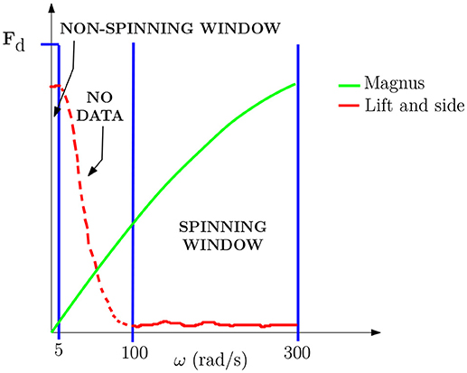
Figure 1. Scheme of the maximum value of lift, side and Magnus forces when varying the angular velocity ω for a given speed V. The y−axis is scaled according to the maximum drag force for the considered velocity. The curves for lift, side and Magnus forces are drawn according to experimental data [8–10]. The missing curve for lift and side forces between spinning and non-spinning windows is because there are no data reported in such range.

The curves in Figure 1 also show the evolution of the study of the types of pitches at this time. Until the beginning of this century, spinning pitches covered most baseball research; therefore, books and compilations of works related to the subject avoided the phenomena present in non-spinning pitches [7]. Nowadays, the interest in non-spinning pitches is resurfacing and there is more information available in books of the present decade, like Cross [6]. However, the new developments and methods for studying non-spinning and intermediate windows are very disconnected, so a new compilation of work on the matter is necessary.

The purpose of this work is to introduce the reader to the diverse existing methodologies for studying the aerodynamic forces in the flight of a baseball, and to discuss the possible ways to complement such studies for future research and applications. All this is based on a literature review of the subject. Each topic begins with a brief derivation of the mathematical model of the respective force; then the model is compared with the results obtained from experimental measures, and a discussion of this is achieved. We have special interest in discussing how the seams affect the aerodynamics of the ball; therefore, the lift force and non-spinning pitches will get more attention.

This review is structured according to the classification of pitches mentioned above. In this way, we begin by presenting the most common mathematical model to describe the movement of a baseball with a concise review of the spinning pitches in section 2. Next, section 3 deals fully with the advances on non-spinning pitches and presents some comments on the boundary layer and the wake of a baseball in motion. Finally, we present a compilation of the existing uses regarding the aerodynamics of baseballs, and outline the research trends of the subject in section 4.

2. Spinning Pitches

In accordance with Figure 1, we define a spinning pitch as any throw, excepting knuckleballs, that has an initial velocity in the range V = [(V_x, V_y, V_z)] ∈ [(−3, 30, −3), (3, 50, 3)] m/s and an initial spin of |ω| = [100, 310] rad/s, which are the values at which baseballs are thrown by professional pitchers when fixing the y−axis in mound-home direction and z−axis perpendicular to the floor, according to the right-hand rule [13]. In this way, some examples of spinning pitches are the curveball, slider, change-up, and the variants of the fastball. The hallmark of this type of pitches is the Magnus force. We begin by describing the drag force in section 2.1, which is present in all types of pitches, with the aim of establishing some basic concepts to introduce the Magnus force.

2.1. The Drag Force

Drag or friction is the force that resists the movement of an arbitrary object. The classical way to derive drag force is by considering that the study of a ball moving through a static medium is equivalent to the one of a static ball with fluid in motion; therefore, V corresponds to the velocity of the fluid, and thus a mathematical formula for the drag of the ball can be obtained from the momentum conservation equation [2, 14]

$\begin{array}{rc}\frac{\partial \text{V}}{\partial t}+(\text{V}·\nabla )\text{V}=-\nabla \left(\frac{p}{\rho }\right)+\text{g},p\equiv \mathrm{\text{pressure}},& (2)\end{array}$

which, in turn, is computed by considering that the air is a Newtonian and incompressible fluid in the Reynold's transport theorem (1); see Ferziger 1996 [2] for the computing of Equation (2). The conservation of mass equation also reduces to

$\begin{array}{rc}\nabla ·\text{V}=0.& (3)\end{array}$

Then, assuming a steady flow the Bernoulli's equation results

$\begin{array}{rc}\frac{1}{2}{V}^2+\frac{p}{\rho }\equiv \mathrm{\text{constant}},& (4)\end{array}$

where we used $\frac{1}{2}\nabla V^2=\text{V}\times (\nabla \times \text{V})+(\text{V}·\nabla )\text{V}$ avoiding the gravitational term [14]. From Bernoulli's Equation (4) the reader can observe that the greatest pressure occurs at points where the velocity equals zero. These points are commonly found on the surface of solid bodies and are usually called stagnation points. For the case of a sphere ball, one stagnation point is present on the front side. The pressure at this point is

$\begin{array}{rc}{p}_{\mathrm{\text{max}}}=p_0+\frac{1}{2}\rho V^2& (5)\end{array}$

where p₀ is the pressure of the fluid at infinity [14, 15]. In this way, the second term is related to the force opposing the motion of the ball, the drag force, and thus drag can be calculated by the difference of pressure between the front and back sides of the ball [2]. However, there are other phenomena affecting the drag. At the corresponding Reynolds number (Re) of a typical throw (10⁴−10⁵) the flow is not steady but turbulent [8, 10, 13, 16, 17]; then the point of separation of the boundary layer moves away from the front of the ball when the ball's velocity increases, making the wake smaller and avoiding a momentum in the reverse direction on the rear of the ball [18, 19].

The approximation of the drag force is done by introducing the sectional transverse area A and a dimensionless coefficient C_d into the second term of the right-hand side in the Equation (5), such that

$\begin{array}{rc}{\text{F}}_d=-\frac{1}{2}\rho C_{d}AV\text{V}.& (6)\end{array}$

where C_d = C_d(V), and then C_d acts in (6) as a fraction of the area A interacting with the air, or in other words, a measure of how aerodynamic the ball is [18, 20, 21].

As a consequence, the study of the drag coefficient (C_d) is so important that it becomes the most effective formula to approximate the drag; therefore, the drag force (F_d) is commonly expressed in terms of C_d. There are two ways to explain the behavior of C_d. On the one hand, there is the drag crisis phenomenon for smooth spheres mentioned in Landau and Lifshitz [14], which indicates that a crisis in the value of C_d can occur at Re~10⁵ (at velocities of 30–40 m/s for a typical baseball). Data shown in Frohlich [22] and Cross [23] fit to such model. On the other hand, from the famous curve of Adair [7] to the recent data obtained by Naito [24], most of the experimental measures suggest a model without drag crisis [6, 17, 25, 26]. This predominance maintains for other sphere balls [23, 27–29] and gives rise to most of the used models to compute the drag force without including the drag crisis phenomenon. There are two models of special interest: the model by Cross [6], from which the drag coefficient can be obtained if the instantaneous ball's velocity at a fixed time is known, and the curve of Adair [7], which approaches to

$\begin{array}{rc}{C}_d(V)=0.29+0.22{\left[1+e^{(V-32.37)/5.2}\right]}^{-1},& (7)\end{array}$

according to Aguirre-López etal. [5]; see Figure 2.

FIGURE 2

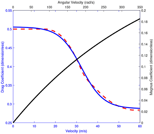
Figure 2. Model of drag and Magnus coefficients. Adair's drag model [7] and the approximation of Aguirre-López et al. [5] showing the sigmoidal decreasing of drag when increasing the velocity of the ball. In turn, the Magnus model (10) presented in Robinson [8] shows that the Magnus coefficient increases when the angular velocity increases. Modified from Aguirre-López et al. [5].

Finally, it is important to mention that the drag has an oscillating dependence on the orientation of the seams. However, for spinning pitches such oscillations average to zero and so they are not considered here. The dependence of C_d on the seams' orientation will be discussed in section 3.1.

2.2. The Magnus Force

Magnus force is the essential characteristic of a spinning pitch, as we mentioned before. The Magnus effect is observed as smooth deflections in the trajectory of a ball. All of us have a clear empirical knowledge of the Magnus effect: large deflections are reached by increasing the spin frequency of the ball. Although this statement is true, the direction of the deflection varies for different configurations of linear velocity V, the angular velocity ω and the ball properties. In fact, for any viewer, the expected direction of the ball's deflection goes on (ω×V), as illustrated in Figure 3. However, a reverse direction of the Magnus force has been reported for smooth balls like those used in soccer [27], and also in smooth spheres simulating baseballs in experiments by Briggs [30], Cross and Lindsey [31]. This phenomenon is commonly called the “anti-Magnus effect” and it is possible only for a range of Re and spin when one side of the smooth ball remains in a laminar flow while the opposite side becomes turbulent. Then, a low pressure region is originated in the turbulent side because it is generally farther to the ball surface than the laminar layer. Thus, the ball moves to the region with lower pressure by conservation of momentum, as illustrated in Figure 3. For a detailed explanation of the causes of the reverse in the direction of Magnus force, the reader is referred to Cross and Lindsey [31]. For a general understanding of the phenomenon, the reverse-Magnus occurs at Re~10⁵ combined with a low speed due to Magnus force Rω (where R is the radius of the ball) compared with the ball's velocity V, such that the spin factor S = Rω/V is in the range 0–0.6.

FIGURE 3

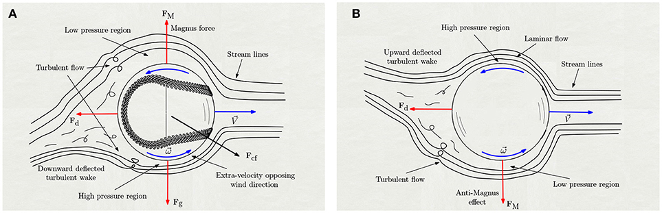
Figure 3. Scheme of the possible ways of causing a Magnus force. (A) The common Magnus force. Modified from Aguirre-López et al. [5]. (B) The reverse Magnus force.

However, the baseball is not smooth and there are no reported studies of an anti-Magnus effect in baseballs. This is because the seams of the ball give to it some roughness that accelerates the separation of the boundary layer in both the up and down sides of the ball. Indeed, the Magnus effect in baseballs' flight arises because one side of the ball offers larger friction than its opposite side, which means that the speed of the main flow of air is larger on the former and as a consequence the lower-pressure region locates at the opposite side, according to the anti-Magnus phenomenon [6–8]; see the schemes in Figure 3. Therefore, the nature of the Magnus force is similar to that of the drag force, due to a difference of pressure. For this reason, Magnus force is commonly written in a similar way as drag force (Equation 6), namely,

$\begin{array}{rc}{F}_{\mathrm{\text{M}}}=\frac{1}{2}\rho A{C}_{\mathrm{\text{M}}}{V}^2,& (8)\end{array}$

for an arbitrary direction of motion, with C_M being the Magnus coefficient. Moreover, in the same system of coordinates to drag force, Equation (8) becomes

$\begin{array}{rc}{\text{F}}_{\mathrm{\text{M}}}=\frac{1}{2}\rho A{C}_{\mathrm{\text{M}}}sin\varphi V^2\widehat{\text{n}},& (9)\end{array}$

where the unit vector $\widehat{\text{n}}=\frac{\omega \times \text{V}}{|\omega \times \text{V}|}$ gives the direction of the resulting linear momentum, ϕ is the angle between ω and V so that (Vsinϕ) is the component of V that contributes to the force [6, 8, 10]. It is important to remark that equation (9) has been widely used to reproduce Magnus force of sport balls and other areas of aerodynamics [32–34], and it has been proved experimentally (for sport balls) only for ϕ = 0, 90 and 180° [8, 10].

The Magnus coefficient C_M is a function of ω and V for arbitrary magnitudes of such variables because Equation (9) depends on both the instantaneous and spin velocities [6, 10, 31]. However, Nathan [17] has reported that C_M behaves independently of V for ω and V values in the range at which spinning pitches are thrown. Moreover, the value of C_M in such range is similar to the Magnus coefficient for other sport balls, and there are some models to calculate its value [8, 30, 35]. Figure 3 shows the model (10):

$\begin{array}{rc}{C}_{\text{M}}(\omega )=3.19\times 10^{-1}\left[1-e^{-2.48\times 10^{-3}\omega }\right],& (10)\end{array}$

which has been used to compute the Magnus force in numerical simulations [5, 8].

2.3. Discussion and Potential Research Trends

In the following items, we summarize and discuss the highlights of the spinning pitches, and also sketch out the potential research trends of the subject:

• Both drag and Magnus forces are commonly expressed in terms of their coefficients, which have information about the object taken from experiments.

• The drag coefficient (7) decreases in a sigmoidal way when the ball's velocity increases. It maintains a value of around C_d = 0.5 up to velocities of 20 m/s, then decreases to C_d = 0.3 in the range of 20–50 m/s (which corresponds to the range of spinning pitches), and maintains that value for larger velocities. In this way, the drag coefficient must be considered as a function of the velocity when computing baseball trajectories.

• There are different ways to measure drag force or estimate the drag coefficient that have not been reported, for instance, by Computational Fluid Dynamics (CFD) or by analyzing the von Karman vortex trails generated by the ball [2, 15]. Both of them could be promising areas of opportunity to characterize the drag, and the aerodynamics of a baseball, in a more comprehensive way.

• Model (9) is the most common formula to approximate the Magnus force. It considers the angular velocity ω as a constant in time (despite torquing forces). This is acceptable since such forces are very small, as mentioned in Ward-Alaways [10].

• The exponential behavior of the Magnus coefficient (10) denotes the effect of ω in the Magnus force. In addition, the model does not depend on the velocity V inside the range of initial conditions for spinning pitches, which simplify the estimation of the Magnus effect.

• The effects of drag and Magnus forces on a spinning pitch can be decoupled and studied separately according to Aguirre-López et al. [5], which could have a lot of applications, such prediction, reconstruction and clustering of trajectories; see section 4.

• Other aspects exist that affect a thrown baseball, such as wind, humidity, etc. However, the study of these effects is more complex and there are few investigations about them [6, 8].

3. Non-spinning Pitches

Non-spinning pitches consist of a specific type of throw: the knuckleball. It contains all combinations for the linear and angular velocities in the ranges V ∈ [20, 40] m/s and ω ∈ [0, 50] rad/s, respectively [36]. Knuckleball pitches are the most interesting throws for aerodynamics because the ball can no longer be considered a sphere since the effect of the seams is significant. However, this is more complex to understand and, therefore, knuckleball studies are fewer than those for spinning pitches.

In this section we discuss the advances in drag force for non-spinning pitches (section 3.1). Then, the description of the models for lift and side forces is presented in section 3.2. An introduction to the modeling of the seams and the boundary layer observations is shown in section 3.3. A compilation of the knuckleball's research and trends is discussed in section 3.4.

3.1. The Drag Force in Non-spinning Pitches

Drag force is different in knuckleballs than in spinning pitches. The drag is approximately constant for a specific velocity in a spinning ball, however, in a knuckleball it is not. As mentioned in section 2.1, the Re of a baseball pitch corresponds to an unsteady flow and then an experimental coefficient must be introduced in the model for the drag force (6). However, when the ball does not spin some vortices are shed from the ball and then the drag oscillates in time. Ferziger and Perić [2] discusses such an effect for a smooth cylinder simulated by CFD. The drag on the cylinder oscillates periodically with a frequency according to the appearance of the vortices such that it has one maximum and one minimum during the formation and shedding of each vortex. Such vortex shedding has also been reported for baseballs in Texier et al. [37], whose effect in lift and side forces will be discussed in section 3.2.

In addition to the variation in time, the drag changes when varying the orientation of the ball. Investigations carried out in the present decade show structured oscillations of drag coefficient despite the turbulence present in the phenomenon. For example, the experiment by Higuchi and Kiura [38] with different configurations of the ball, namely, the four-seam (4S), the two-seam (2S) and an arbitrary orientation of the ball¹. They found the largest variation in oscillations for the 4S orientation, which is about twice as large as the case of the 2S orientation and around four times that of the arbitrary orientation. The shape of the oscillations in the 4S orientation is maintained for ball velocities in the range of 16–30 m/s.

Similar average variations for C_d have been reported by Alam et al. [25] in studies of the drag force for Major League Baseball (MLB) and National Collegiate Athletic Association (NCAA) baseballs and softballs. They reported lower variations in C_d values for NCAA than for MLB baseballs at different ball orientations, which suggests a dependence on the height of the seams (1.5 mm for NCAA and 1mm for MLB balls). At first glance, the idea seems to be solid because a larger “extra-obstacle” should cause a corresponding “extra-drag” in the fluid. Even more, this is supported by the results of Kensrud et al. [39], who analyzes hit balls with different heights of seams and found that balls with smaller seams reach larger distances, which indicates a lower drag.

Finally, it is important to remark that commonly C_d decreases with increasing V for baseballs, softballs, cricket balls and smooth spheres. In the case of baseballs, the value of C_d decreases from ~0.6 to ~0.4 dimensionless units [25, 32].

3.2. The Lift and Side Forces

The main reason for which knuckleball pitches are much more unpredictable than spinning pitches is because of lift and side forces². Similar to the drag and Magnus forces, lift force is produced by an imbalance in pressure and then it is proportional in magnitude to the square of the ball velocity [11, 40], so that

$\begin{array}{ll}{F}_L=\frac{1}{2}\rho C_{L}A{V}^2.& (11)\end{array}$

However, the behavior of the lift coefficient (C_L) is not like C_d or C_M but it varies with the angle of attack θ of the ball. Figure 4 shows how unpredictable a knuckleball can be, even for the most symmetric ball orientations (4S and 2S). Results of Borg and Morrisey [36] show four cycles in C_L for the 4S orientation, each one with a period of 90°, with a semi-sinusoidal behavior and ringlets at the end of a cycle. This means that a variation of ~22.5° in smooth-angle zones may or may not produce a maximum/minimum lift; instead, a variation of only ~10° in the zone of ringlets can produce any type of motion. In addition to such complexity for a strictly non-spinning ball, in practice it is difficult for a ball to travel without rotating since a little spin is induced by contact from the air with the seams [12, 37]. As a consequence, the ball's trajectory could have an apparent erratic motion whereas the map of balls passing through the home plate in a real pitch is seen as random when varying θ [40]. All of this makes it difficult to compute a model that may accurately reproduce the trajectory of a knuckleball with any orientation.

FIGURE 4

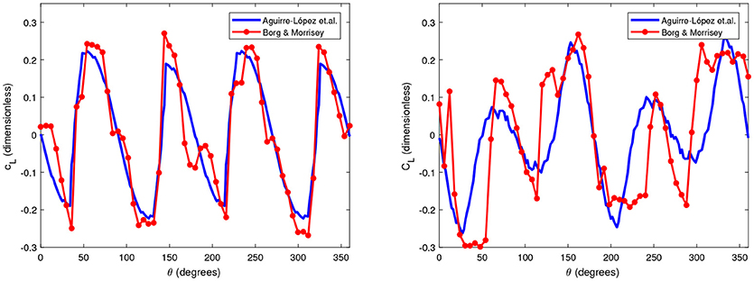
Figure 4. Experimental data [36] and model [41] of C_L as a function of the attack angle θ for 4S (A) 2S (B) balls. Modified from Aguirre-López et al. [41].

It is important to mention that there is controversy in the causes that originate the lift force. It is evident that the asymmetry of the seams plays a fundamental role in causing such force. According to Watts and Sawyer [11] and Mehta [12], there are two possible ways to produce a lift force on a baseball: for many years, the classical hypothesis stated that the lift is produced not only by the seams but by the shedding of vortices that occurs at the rear side of the ball. All of these interact in a complex way, as mentioned in Ferziger and Perić [2], Watts and Sawyer [11], and Mehta [12]. On the other hand, and according to Texier et al. [37], there is the possibility that the lift force may be originated only by the perturbations at the front side of the ball. This means that the seams produce the total lift of the ball, especially those located at the separation or critical points of the boundary layer at 52, 140, 220, and 310° [12, 36]; this will be addressed in detail in section 3.3. Texier calculated that the force produced by the vortices at Strohual numbers (St) of St~0.2 is significantly lower than the magnitude of the lift measured in experiments, so that it practically does not contribute to lift. More information about lift force in ball sports can be found in investigations by Mehta [12], Hong et al. [42], and Murakami et al. [43].

3.3. The Seams and the Boundary Layer

The manner in which the seams affect the boundary layer is very sensitive to small changes between seams. As commented by Borg and Morrisey [36], when a seam is located near the natural separation angle (the angle of separation of a smooth ball), it can induce turbulence and consequently provoke a delay in the separation of the boundary layer; in turn, the seam can force the separation to occur and cause an advance in the separation angle. Such effects are seen in the sudden changes in the values of the lift coefficient for a 4S orientation. For a smooth ball, a sinusoidal shape of C_L would be expected, in a similar way to the lift coefficient reported for a smooth cylinder by Ferziger and Perić [2]. However, Figure 4 suggests a quasi-periodic behavior for C_L for 4S balls, with fast changes in magnitude and direction at 52, 140, 220 and 310°, as observed by Watts and Sawyer [11]. This is because the separation point is located around such degrees and then it advances or delays with a little variation in the stitch position.

Experiments by Higuchi and Kiura [38] show that a variation of only one degree (36 to 37°) in the stitch position causes a sudden separation. Moreover, they reported that the balls are more susceptible to hysteresis (including induced rotation) at the zones of separation. For 4S balls and Re above 1.5 × 10⁵, the ball is sensitive to the initial rotation, namely, spins of 5 rad/s become 10.5 rad/s, increasing linearly and having a spin limit of 18.9 rad/s even for Re above 2 × 10⁵. In turn, for 2S balls they found that the oscillation frequency is constant over Re ∈ [1.9 × 10⁵, 4.6 × 10⁵]. As a consequence of the induced rotation, the phenomenon becomes more unpredictable because the separation point moves forward or backward at every moment of time. This is the reason why the throws inside the intermediate window in Figure 1 are the most difficult to study. We invite the reader to consult the research of Higuchi and Kiura [38] for detailed observations of the boundary layer.

To end the collection of the advances on knuckleballs, it is important to mention the phenomenological model proposed by Aguirre-López et al. [41] for computing the lift coefficient. It consists of computing a super-imposition of the forces produced by the vortex shedding and each stitch, so that

$\begin{array}{l}{C}_L(\theta )=a_{0}sin(4\theta -\pi )+a_1{\displaystyle \sum _{i=1}^n}[sin\left(\frac{\left|\right|{\text{s}}_i-\text{p}\left|\right|\pi }{2d}+\pi /2\right)·\\ \mathrm{\text{ sgn}}(p^{*}-s_i^{*})],& (12)\end{array}$

where C_L = C_L(θ) is now a function of the angle of attack of the ball, the first term in the right-hand side is the force caused by the vortex shedding and the term ∑(·) is the sum of forces produced by the seams, p is the stagnation point, s_i is the position of the i-th stitch, $s_i^{*}$ and p* are the z−components of s_i and p, respectively, and a₀ and a₁ are weight coefficients. Therefore, each stitch in model (12) produces a force whose magnitude decreases smoothly when the stitch moves away from the stagnation point and takes into account the symmetry on the z-axis by introducing the sign function sgn(·). Thus, despite the fact that model (12) does not consider effects of hysteresis and high sensitivity to perturbations at the separation point, it fits the experimental data of Borg and Morrisey [36] for 4S and 2S orientations, as shown in Figure 4. Model (12) opens the door to future research on how the seams and the vortex shedding affect the lift force.

3.4. Discussion and Potential Research Trends

Here we summarize and discuss the highlights of the non-spinning pitches and outline potential research trends of knuckleballs pitches as follows:

• The structure of the oscillations of the drag coefficient depends on the orientation of the ball, whereas the height of the seams increases the magnitude of the drag.

• The value of C_D decreases from 0.6 to 0.4 units when increasing V.

• The lift coefficient oscillates every 90°, with a quasi-periodic behavior for 4S balls, which is related to the effect of the seams. In fact, values of C_L for 2S balls oscillate every 180°, with an inversion every cycle [36, 38].

• The origin of lift force is not well understood. On the one hand, seams could cause the total lift, and on the other hand, a sum of both the seams and the vortex shedding could be the source of it [11, 36, 37].

• Observations on the boundary layer suggest that the lift force is more susceptible to perturbations at some angles, including 52, 140, 220, and 310° for 4S balls. Hysteresis is partly responsible for this [38].

• We consider that simulations using CFD techniques could disentangle the causes that produce the lift force.

• In addition to the last point, CFD simulations could help to improve the model (12) or propose a variation of it that involves the susceptible zones of the separation point, and extend the model to arbitrary orientations.

4. Applications

As the reader may suppose, there are many ways to make useful the information compiled in sections 2 and 3. And, indeed, baseball studies have been the basis of numerous technologies on the matter, specifically those ones about spinning pitches. We finalize this work with a brief summary of the main applications of the aerodynamic forces on baseballs. Section 4.1 is focused on the studies related to baseball's trajectories. In turn, section 4.2 talks about the complementary applications including the best known of them: the PITCHf/x algorithm.

4.1. Prediction and Reconstruction of Trajectories

4.1.1. The Simulation Problem

The most simple use of aerodynamic forces is the simulation or prediction of trajectories. A simulation of a baseball pitch is frequently carried out by using the Equations (6) and (9) along with gravity to compute a model of forces as:

$\begin{array}{rc}m\stackrel{·}{\text{V}}={\text{F}}_d+{\text{F}}_M+m\text{g},& (13)\end{array}$

which can be solved numerically by Runge-Kutta-4 or other integration methods, whereas drag and Magnus coefficients can be computed by Equations (7) and (10) or similar approximations [6, 44]. The simulations could become more realistic by including eventual forces in the model (13). An example of this is the model of Robinson and Robinson [8], which adds a constant in wind to the ball velocity so that V′ is redefined as (V′ = V+W), where W is the wind velocity.

In turn, simulations of baseball trajectories are commonly applied to some sport and technology areas such as in video games [45], baseball machines [10] as well as for instruction for baseball players. The last one is the main reason for which research on knuckleballs is a topic of special interest.

4.1.2. The Reconstruction Problem

The counterpart of simulation is the reconstruction of trajectories. In these works, there is no possibility to give the initial conditions of a pitch and obtain the trajectory but the trajectory must be extracted, tracking or reconstructed only by a set of 3D or 4D (space plus time) points belonging to the trajectory. Such data points are commonly recorded by baseball broadcast videos and/or images of real games; therefore, the trajectory obtained is used for the replay in television.

Various methodologies have been reported for extracting or tracking the trajectory. Most of them use types of diverse filters like color, position, size and shape [46–48], and others [49, 50] select possible trajectories. Then the chosen trajectories are compared with the model (13) so that, if the resulting trajectory does not agree with the model, then it is discarded and a new one is needed. Takahashi et al.'s investigation [47] also deals with classifying the type of pitch by relating a total of 36 features, including the shape and speed calculated from the ball trajectory data and the ball speed from the screen display. They report an accuracy of ~89% with their methodology.

The methodologies that deal with a “direct” reconstruction are based on the use of the equations of motion. Shum and Komura [51] and Miyata et al. [52] use color filtering for detecting 2D candidate trajectories. Then, Shum and Komura estimate the depth of the ball in the scene by introducing a model (13). In turn, Miyata et al. [52] chose one candidate by fitting a uniformly accelerated motion model [similar to model (13)] and finally, they use multiple cameras calibrated temporally and geometrically to obtain a 3D trajectory. On the other hand, Aguirre-López et al. [5] developed an algorithm that directly solves the model (13) in two interrelated parts by decoupling the Magnus force from the equations of motion, using the Newton-Raphson method when knowing three points of the trajectory. They reported absolute error values of ~0.1 mm between simulated and reconstructed trajectories. Finally, Kagan and Nathan [53] have developed a software called the trajectory calculator, which is similar in operation to that of Aguirre-López et al. [5] but with simpler assumptions. The results are less accurate but it is a good tool to start in the subject. The trajectory calculator can be downloaded directly at [54].

4.2. The PITCHf/x Algorithm and Clustering

The second part of the application deals with problems related to the classification of trajectories, among which the PITCHf/x algorithm is the most popular and accurate reported method in research and in the world of baseball. The algorithm (including new versions and software packages) has been consolidated as a powerful tool in the area of pitch classifications [55, 56].

The PITCHf/x algorithm consists of two parts. The first one involves reconstructing trajectories by estimating the coefficients C_d, C_M and the spin axis ϕ (the angle between y−axis and ω) using non-linear least-squares fitting with the Levenberg-Marquardt algorithm. Nathan [55] reports very good adjustments; indeed, root-mean-square deviations of the fitted trajectory of around 1 mm in each dimension. The second (and the main) part of the work deals with the classification of pitches. The classification is based on (V vs. ϕ) and (ω vs. ϕ) graphics. As a result, the types of pitches are arranged in clusters in polar scatter plots and scatter plots of the deflection of the ball at home. Pane [57] carried out an interesting cluster analysis from the results of Nathan [55] based on PITCHf/x. The research on the topic continues.

5.Ethics Statement

We express our gratitude to Elsevier for the permission to reuse a modified version of the copyrighted Figures 2, 3a, 4 in the present paper. Order numbers: 4511461494464 and 4511510076028.

6. Author Contributions

GE and OD-H contributed to the design and discussion of this document. MA-L contributed to the design and writing of this document. FH-Z contributed to the discussion and writing of this document. JM-C and F-JA contributed to the discussion of this document and as advisor.

Conflict of Interest Statement

The authors declare that the research was conducted in the absence of any commercial or financial relationships that could be construed as a potential conflict of interest.

Acknowledgments

FH-Z thanks CONACyT, Cátedra 873.

Footnotes

1. ^A detailed explanation of the typical baseball orientations can be found in Borg and Morrisey [36].

2. ^From this point on we will use the term “lift force” for referring to both lift and side forces because both are equivalent, excluding gravity.

References

1. White FM. Fluid Mechanics. New York, NY: McGraw Hill (2003).

Google Scholar

2. Ferziger JH, Perić M. Computational Methods for Fluid Dynamics. Berlin: Springer (1996).

Google Scholar

3. Fitzpatrick R. Theoretical Fluid Mechanics. Available online at: http://farside.ph.utexas.edu/teaching/336L/Fluid.pdf

4. Robinson G, Robinson I. Are inertial forces ever of significance in cricket, golf and other sports? Phys Scripta (2017) 92:043001. doi: 10.1088/1402-4896/aa634e

CrossRef Full Text | Google Scholar

5. Aguirre-López MA, Morales-Castillo J, Díaz-Hernández O, Escalera Santos GJ, Almaguer F-J. Trajectories reconstruction of spinning baseball pitches by three-point-based algorithm. Appl Math Comput. (2018) 319:2–12. doi: 10.1016/j.amc.2017.01.016

CrossRef Full Text | Google Scholar

6. Cross R. Physics of Baseball & Softball. New York, NY: Springer (2011).

Google Scholar

7. Adair RK. The Physics of Baseball. New York, NY: Harper-Collins Publishers (2002).

Google Scholar

8. Robinson G, Robinson I. The motion of an arbitrarily rotating spherical projectile and its application to ball games. Phys Scripta (2014) 88:018101. doi: 10.1088/0031-8949/88/01/018101

CrossRef Full Text | Google Scholar

9. Cross R. Information About Knuckleballs. Available online at: http://www.physics.usyd.edu.au/ cross/KNUCKLEBALLS.htm

10. Ward-Alaways L. Aerodynamics of the Curve-Ball: an Investigation of the Effects of Angular Velocity on Baseball Trajectories, Philosophy Doctoral Thesis, University of California (1998).

11. Watts RG, Sawyer E. Aerodynamics of a knuckleball. Am J Phys. (1975) 43:11. doi: 10.1119/1.10020

CrossRef Full Text | Google Scholar

12. Mehta RD. Aerodynamics of sports balls. Annu Rev Fluid Mech. (1985) 17:151–89. doi: 10.1146/annurev.fl.17.010185.001055

CrossRef Full Text | Google Scholar

13. MLB Games (2015). Statistics of 2015 MLB Games. Available online at: http://m.mlb.com/news/article/160896926/statcast-spin-rate-compared-to-velocity

14. Landau LD, Lifshitz EM. Fluid Mechanics. Elsevier (1987).

15. Prandtl L, Tietjens OG. Applied hydro- and aeromechanics. USA: Dover (2016).

Google Scholar

16. Official Baseball Rules (2015). Available online at: http://mlb.mlb.com/mlb/downloads/y2015/official_baseball_rules.pdf

17. Nathan AM. The effect of Spin on the Flight of a Baseball. Am J Phys. (2008) 76:119–24. doi: 10.1119/1.2805242

CrossRef Full Text | Google Scholar

18. Watts RG, Moore G. The drag force on an american football. Am J Phys. (2003) 71:791–3. doi: 10.1119/1.1578065

CrossRef Full Text | Google Scholar

19. Luthander S, Ryberg A. Experimentelle Untersuchungen uber den Luftwiderstand bei einer um ein mit der Windrichtung parallelen Achse roteirenden Kugel. Phys Z (1935) 36:552–8.

Google Scholar

20. Daish CB. The Physics of Ball Games. London: The English Universities Press (1972).

Google Scholar

21. Hennekam W. The speed of a cyclist. Phys Educ. (1990) 25:141–6. doi: 10.1088/0031-9120/25/3/001

CrossRef Full Text | Google Scholar

22. Frohlich C. Aerodynamic drag crisis and its possible effect on the flight of baseballs. Am J Phys. (1984) 52:325–34. doi: 10.1119/1.13883

CrossRef Full Text | Google Scholar

23. Cross R. Effects of turbulence on the drag force on a golf ball. Eur J Phys. (2016) 37:054001. doi: 10.1088/0143-0807/37/5/054001

CrossRef Full Text | Google Scholar

24. Naito K, Hong S, Koido M, Nakayama M, Sakamoto K, Asai T. Effect of seam characteristics on critical Reynolds number in footballs. Mech Eng J. (2018) 17:00369.

Google Scholar

25. Alam F, Ho H, Smith L, Subic A, Chowdhury H, Kumar A. A study of baseball and softball aerodynamics. Proc Eng. (2012) 34:86–91. doi: 10.1016/j.proeng.2012.04.016

CrossRef Full Text | Google Scholar

26. Kensrud JR, Smith LV. In situ drag measurements of sports balls. Proc Eng. (2010) 2:2437–42. doi: 10.1016/j.proeng.2010.04.012

CrossRef Full Text | Google Scholar

27. Kray T, Franke J, Frank W. Magnus effect on a rotating soccerball at high Reynolds numbers. J Wind Eng Indust Aerodyn. (2014) 124:46–53. doi: 10.1016/j.jweia.2013.10.010

CrossRef Full Text | Google Scholar

28. Cross R. Vertical impact of a sphere falling into water. Phys Teacher (2016) 54:153–5. doi: 10.1119/1.4942136

CrossRef Full Text | Google Scholar

29. Goff JE. A review of recent research into aerodynamics of sport projectiles. Sports Eng. (2013) 16:137–54. doi: 10.1007/s12283-013-0117-z

CrossRef Full Text | Google Scholar

30. Briggs LJ. Effect of spin and speed on the lateral deflection (curve) of a baseball; and the magnus effect for smooth spheres. Am J Phys. (1959) 27:589–96. doi: 10.1119/1.1934921

CrossRef Full Text | Google Scholar

31. Cross R, Lindsey C. Measurements of drag and lift on smooth balls in flight. Eur J Phys. (2017) 38:044002. doi: 10.1088/1361-6404/aa6e44

CrossRef Full Text | Google Scholar

32. Sayers AT. Hill A. Aerodynamics of a cricket ball. J Wind Eng Indust Aerodyn. (1999) 79:169–82. doi: 10.1016/S0167-6105(97)00299-7

CrossRef Full Text | Google Scholar

33. Goodwill SR, Chin SB, Haake SJ. Aerodynamics of spinning and non-spinning tennis balls. J Wind Eng Indust Aerodyn. (2004) 92:935–58. doi: 10.1016/j.jweia.2004.05.004

CrossRef Full Text | Google Scholar

34. Lorentz RD. Spinning Flight. Dynamics of Frisbees, Boomerangs, Samaras, and Skipping Stones. New York, NY: Springer (2006).

Google Scholar

35. Robinson G, Robinson I. Reply to Comment on ‘The motion of an arbitrarily rotating spherical projectile and its application to ball games’. Phys Scripta (2014) 89:5. doi: 10.1088/0031-8949/89/6/067002

CrossRef Full Text | Google Scholar

36. Borg JP, Morrisey MP. Aerodynamics of the knuckleball pitch: experimental measurements on slowly rotating baseballs. Am J Phys. (2014) 82:921.doi: 10.1119/1.4885341

CrossRef Full Text | Google Scholar

37. Texier BD, Cohen C, Quéré D, Clanet C. Physics of knuckleballs. N J Phys. (2016) 18:073027. doi: 10.1088/1367-2630/18/7/073027

CrossRef Full Text | Google Scholar

38. Higuchi H, Kiura T. Aerodynamics of knuckle ball: flow-structure interaction problem on a pitched baseball without spin. J Fluids Struct. (2012) 32:65–77. doi: 10.1016/j.jfluidstructs.2012.01.004

CrossRef Full Text | Google Scholar

39. Kensrud JR, Smith LV, Nathan A, Nevins D. Relating baseball seam height to carry distance. Proc Eng. (2015) 112:406–11. doi: 10.1016/j.proeng.2015.07.216

CrossRef Full Text | Google Scholar

40. Nathan AM. Analysis of knuckleball trajectories. Proc Eng. (2012) 34:116–21. doi: 10.1016/j.proeng.2012.04.021

CrossRef Full Text | Google Scholar

41. Aguirre-López MA, Díaz-Hernández O, Almaguer F-J, Morales-Castillo J, Escalera Santos GJ. A phenomenological model for the aerodynamics of the knuckleball. Appl Math Comput. (2017) 311:58–65. doi: 10.1016/j.amc.2017.05.001

CrossRef Full Text | Google Scholar

42. Hong S, Chung C, Nakayama M, Asai T. Unsteady aerodynamic force on a knuckleball in soccer. Proc Eng. (2010) 2:2455–60. doi: 10.1016/j.proeng.2010.04.015

CrossRef Full Text | Google Scholar

43. Murakami M, Seo K, Kondoh M, Iwai Y. Wind tunnel measurement and flow visualisation of soccer ball knuckle effect. Sports Eng. (2012) 15:29–40. doi: 10.1007/s12283-012-0085-8

CrossRef Full Text | Google Scholar

44. Clark JM, Greer ML, Semon MD. Modeling pitch trajectories in fastpitch softball. Sports Eng. (2015) 18:157–64. doi: 10.1007/s12283-015-0176-4

CrossRef Full Text | Google Scholar

45. Syamsuddin MR, Kwon YM. Simulation of baseball pitching and hitting on virtual world. Phys Scripta (2011) 663–667.

Google Scholar

46. Chu WT, Wang CW, Wu JL. Extraction of baseball trajectory and physics-based validation for single-view baseball video sequences. Int Cong Multimedia Expo (2006) 1813–16. doi: 10.1109/ICME.2006.262905

CrossRef Full Text | Google Scholar

47. Takahashi M, Fujii M, Yagi N. Automatic pitch type recognition from baseball broadcast videos. Int Symp Multimedia (2008) 15–22.

Google Scholar

48. Chang P, Han M, Gong Y. Extract highlights from baseball game video with hidden Markov models. In: International Congress of Imaging Processing, Vol. 1, (2002). p. 609–12.

Google Scholar

49. Hung MH, Hsieh CH. Event detection of broadcast baseball videos. Trans Circ Syst Video Technol. (2008) 18:1713–26.

Google Scholar

50. Guéziec A. Tracking pitches for broadcast television. Computer (2002). doi: 10.1109/2.989928

CrossRef Full Text | Google Scholar

51. Shum H, Komura T. A spatiotemporal approach to extract the 3D trajectory of the baseball from a single view video sequence. In: International Conference on Multimedia and Expo, Vol. 3 (2004) p. 1583–86. doi: 10.1109/ICME.2004.1394551

CrossRef Full Text | Google Scholar

52. Miyata S, Saito H, Takahashi K, Mikami D, Isogawa M, Kimata H. Ball 3D trajectory reconstruction without preliminary temporal and geometrical camera calibration. In: IEEE Conference on Computer Vision and Pattern Recognition Workshops (2017).

Google Scholar

53. Kagan D, Nathan AM. Statcast and the baseball trajectory calculator. Phys Teach. (2017) 55:134. doi: 10.1119/1.4976652

CrossRef Full Text | Google Scholar

54. Nathan AM. The Trajectory Calculator. Available online at: http://baseball.physics.illinois.edu/trajectory-calculator-old.html

55. Nathan AM. Analysis of PITCHf/x Pitched Baseball Trajectories. (2008). Available online at: https://www.researchgate.net/publication/228563555_Analysis_of_PITCHfx_Pitched_Baseball_Trajectories

56. Sievert C. Taming PITCHf/x Data with XML2R and pitchRx. R J. (2014) 6:5–19.

Google Scholar

57. Pane MA. Trouble With the Curve: Identifying Clusters of MLB Pitchers using Improved Pitch Classification Techniques, Philosophy Doctoral Thesis, Carnegie Mellon University (2013).