On the Influence of Production Technologies and Savings Propensities on Economic Growth. Findings Considering a Solow's Type Growth Model

1. Introduction

What explains changes on the gross domestic product (GDP) of a country? Can investments increase it? Why is GDP stagnant in non-developed or developing economies? Neoclassical growth theory provides a theoretical framework to explain the long run behavior of an economy by considering three driving forces: capital, labor and technology. In his essay A Contribution to the Theory of Economic Growth, the Nobel Prize-winning [2] rejected the so called Harrod-Domar assumption (see [3, 4]) of fixed proportions between production's inputs and supposed the possibility of substitution between capital and labor. He discussed how the long run behavior of physical capital is influenced by the structure of production functions (technologies) and the income distribution. With his contribution, Solow founded the neoclassical growth theory: growth models á la Solow describe the evolution over time of the studied variables and they can be formalized in continuous as well as discrete time. In discrete time, i.e., t ∈ ℕ, a production function F is a law that relates the GDP of a nation at time t, Y_t, to the amount of capital K_t and labor L_t utilized by the economy as well as to the technological progress A, i.e., Y_t: = AF(K_t, L_t). When a production function satisfies Constant Returns to Scale (an increase in inputs determines an increase in output of the same proportion) then the technology may be written in intensive from as y_t = Af(k_t) where $y_t:=\frac{Y_t}{L_t}$ and $k_t:=\frac{K_t}{L_t}$ are, respectively output and capital per worker at time t. Solow assumed capital per capita evolves over time following the rule:

$\begin{array}{cc}\begin{array}{r}{k}_{t+1}=\frac{1}{1+n}\left[(1-\delta )k_t+sf(k_t)\right]\end{array}& (1)\end{array}$

where n ≥ 0 is the labor force growth rate, δ ∈ (0, 1] is the depreciation rate of capital, and s ∈ (0, 1) is the saving rate. Therefore, the amount of capital at time t + 1 depends on the existent (and depreciated) capital at time t, on the saving behavior of the nation (the amount of production that is invested) and on the growth of the labor force. Although the model has been widely used to analyse fundamental issues of macroeconomics, it always predicts convergence to a steady state and, hence, it precludes the possibility of cycles to emerge. Moreover, it doesn't take into account that workers and shareholders have different saving propensities (see [5–7]). In order to analyse what influences boom and bust periods and to study how different saving behaviors affect growth, the Solow model has been extended: when different savings behaviors for workers and shareholders are considered, the aggregate saving rate is non-constant and depends on income distribution, being given by

$\begin{array}{cc}\begin{array}{r}s(k_t)=\frac{s_{w}w(k_t)+s_r\pi (k_t)}{f(k_t)},\end{array}& (2)\end{array}$

where s_w ∈ (0, 1) and s_r ∈ (0, 1) are, respectively the saving rates of workers and shareholders, w(k_t) is the wage of a worker and π(k_t) is the income per worker of a shareholder. As an immediate implication, even under the usual neoclassical condition on production, the model may generate multiple equilibria and fluctuations. Following previous considerations, Böhm and Kaas [1] assumed different saving rates in a Solow's type model while considering a generic production function in intensive form. In order to study the evolution of capital per capita, they proposed the BK model

$\begin{array}{cc}\begin{array}{r}{k}_{t+1}=\varphi (k_t):=\frac{1}{1+n}\left[(1-\delta )k_t+s_{w}w(k_t)+s_r\pi (k_t)\right]\end{array}& (3)\end{array}$

that describes the growth dynamics of an economy over time in the neoclassical framework, with different saving propensities between workers and shareholders. Neoclassical growth theory usually assumes that input factors are paid their marginal product, so that

$\begin{array}{cc}\begin{array}{r}\pi (k_t):=k_t{f}^{\prime }(k_t)\mathrm{\text{and}}w(k_t):=f(k_t)-k_t{f}^{\prime }(k_t).\end{array}& (4)\end{array}$

The production function f(k_t) may be classified depending on the elasticity of substitution (ES) between capital and labor, usually denoted by σ. The ES measures the ease with which inputs may be substituted in production while preserving a given level of output. For any continuous and twice differentiable production function, the elasticity of substitution has been defined by Sato and Hoffman [8] as

$\begin{array}{cc}\begin{array}{r}\sigma =-\frac{f^{\prime }(k_t)\left[f(k_t)-k_t{f}^{\prime }(k_t)\right]}{k_{t}f(k_t)f^{\prime \prime }(k_t)}.\end{array}& (5)\end{array}$

A linear production function implies perfect substitution between capital and labor, consequently, σ = +∞. In contrast, when the production function has fixed proportions, input factors are complements and not substitutes, hence, σ = 0. When σ is constant for any combination of the input factors, the technology is said to have Constant Elasticity of Substitution (CES). Conversely, when the ratio between capital and labor influences the value of σ, the technology is said with Variable Elasticity of Substitution (VES). The long run behavior of an economy described by the BK model is qualitatively determined by the saving propensities of worker and shareholders as well as by the implied production function (whether CES or VES). In this work, we review the literature about Constant and Variable ES production functions as ingredients of the BK model and their influence on the evolution of an economy over time. The aim is to understand how fluctuations or complex evolutions of capital per capita are generated and the impact of the implied technologies on the different evolutions of non-developed, developing and developed countries. The paper is structured as follows. Section 2 discusses the influence of different saving propensities on growth when the BK model is considered, and presents findings about the complex dynamics emerging from the BK model for a generic production function satisfying weak Inada conditions. Section 3 analyse the influences of different technologies on growth dynamics, and a summary about the influence of each considered factor is given in section 4. Section 5 concludes the work.

2. An Overview on the BK Model

We initially review the BK model in its original form without specifying the implied technology and, consequently, while considering a generic production function f(k_t). Recall that the BK model is given by

$\begin{array}{cc}\begin{array}{r}{k}_{t+1}=\varphi (k_t):=\frac{1}{1+n}\left[(1-\delta )k_t+s_{w}w(k_t)+s_r\pi (k_t)\right]\end{array}& (6)\end{array}$

and its formulation implies that capital per capita evolves over time depending on technology f(k_t), on the labor force growth rate n≥0, and on the saving propensities of workers and shareholder, respectively s_w ∈ (0, 1) and s_r ∈ (0, 1).

2.1. Bounds of Growth

Notice that macroeconomic theories traditionally assume higher values of saving propensity for shareholder relative to that of workers (see [7]). Therefore, in this section, we consider the economically meaningful condition s_r>s_w¹. It is worthwhile to report the results obtained by Grassetti et al. [9] concerning the influence of saving behaviors on the evolution over time of capital per capita. In particular, the authors provide upper and lower bounds for growth and analyse how different economic policies that condition saving propensities would modify the evolution of capital for non-developed, developing and developed countries. The basic reasoning is the following. Consider the functions

$\begin{array}{cc}\begin{array}{r}{\varphi }_w(k_t):=\frac{1}{1+n}\left[(1-\delta )k_t+s_{w}f(k_t)\right]\end{array}& (7)\end{array}$

and

$\begin{array}{cc}\begin{array}{r}{\widehat{\varphi }}_{w,r}(k_t):={\varphi }_w(k_t)+\frac{s_r-s_w}{1+n}\widehat{k}{f}^{\prime }(\widehat{k})\end{array}& (8)\end{array}$

where $\widehat{k}$ is the value of capital per capita for which the capital income π reaches its maximum. When the used technology is described by a non-linear function, an explicit analysis of the dynamics generated by map ϕ (given by Equation 6) may be difficult and equilibria as well as growth paths may not be given explicitly. Functions ${\widehat{\varphi }}_{w,r}(k_t)$ and ϕ_w(k_t) are clearly easier to analyse than the initial ϕ. Since we assume the savings rate of shareholders is higher than that of workers, the upper bound of the capital per capita level, at any time, is given by ${\widehat{\varphi }}_{w,r}(k_t)$ while the lower bound is given by ϕ_w(k_t).

Thanks to this simple intuition on bounds (see Figure 1 for a graphical representation), a good approximation can be given for the evolution of capital per capita. Moreover, economic policies designed to increase the lower level the economy can reach during fluctuations can be discussed: the lower bound of the capital accumulation depends only on the saving propensity of workers while the saving behavior of shareholders influences the maximum feasible growth. Since ϕ_w(k_t) is the lower bound of GDP, and given that $\frac{\partial {\varphi }_w(k_t)}{\partial s_w}>0$ and ∀k_t≥0, a higher saving rate of workers implies a higher bound from below for the economy. Therefore, an economic policy intended to increase the saving behavior of workers may increase the minimum level an economy may reach during fluctuations. Consider now the upper bound ${\widehat{\varphi }}_{w,r}(k_t)$. The first derivative with respect to s_w may be written as

$\begin{array}{cc}\begin{array}{r}\frac{\partial {\widehat{\varphi }}_{w,r}(k_t)}{\partial s_w}=\frac{f(k_t)-\widehat{k}{f}^{\prime }(\widehat{k})}{1+n}\end{array}& (9)\end{array}$

where, by definition, f(k_t) is increasing and $\widehat{k}$ is the level of capital for which the capital income reaches its maximum. It follows that the level of production influences this bound. Precisely, when the maximum income of a shareholder is higher than the production per capita level, the upper bound of the economy is negatively correlated with the saving behavior of workers and it is positively correlated otherwise. Since GDP is a measure of development for a nation, it is possible to conclude that an increase in s_w would increase the upper bound of countries in which production is sufficiently high, while it would decrease that of non-developed economies. In order to raise both bounds of the growth path for a developed economy, a policy maker could increase the saving propensity of workers. The same economic policy directed at a developing country would decrease the range of oscillations during boom and bust periods.

FIGURE 1

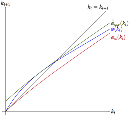
Figure 1. Map ϕ (in blue) and its bounds ${\widehat{\varphi }}_{w,r}(k_t)$ and ϕ_w(k_t).

2.2. Weak Inada Conditions in BK Model

In their work, Böhm and Kaas [1] relaxed the assumption on production and gave necessary conditions for a generic production function satisfying the weak Inada conditions (see [10]) to generate chaos. Weak Inada conditions for a generic production function f(k_t) in intensive form are given by

$\begin{array}{cc}\begin{array}{r}{\displaystyle \underset{k_t\to 0}{lim}}\frac{f(k_t)}{k_t}=\infty \mathrm{\text{and}}{\displaystyle \underset{k_t\to \infty }{lim}}\frac{f(k_t)}{k_t}=0\end{array}& (10)\end{array}$

and they imply unrestricted productivity of capital. Considering this type of technology, the authors gave necessary conditions for the existence of cycles and chaotic dynamics, as summarized in the following Remark.

Remark 2.1. Consider a production function f:ℝ₊ → ℝ₊, mapping capital per worker k_t into output per worker y_t, satisfying the weak Inada condition given by Equation (10). Then the BK model (Equation 6) may generate cyclical behavior iff

$s_r>s_w\mathit{\text{or }}{E}_{f^{\prime }}(k_t):=\frac{k_t{f}^{\prime \prime }(k_t)}{f^{\prime }(k_t)}<-1.$

Moreover, ∀s_w = s_r − ϵ, ϵ > 0, ∃f such that map (Equation 6) generates topological chaos. (For proof see [1].)

Conditions given in Remark 2.1 are related to income distribution: for a production function satisfying (Equation 10), capital income $k_t{f}^{\prime }(k_t)$ decreases with increasing capital stock when $E_{f^{\prime }}(k_t)<-1$. Cyclical behavior may be generated only if shareholders save more than workers or if the curvature of f is sufficiently small in absolute value (notice that the $E_{f^{\prime }}(k_t)$ measures the curvature of the production function f). Lastly, given previous assumptions, complex dynamics arise when the saving behavior of workers and shareholders are only slightly different. In order to asses the existence of complex behavior in growth dynamics, a wider range of production functions have been studied in the BK model, as we report in next section.

3. Technologies, Elasticity of Substitution and Growth Dynamics

So far we have considered how the changes in saving behaviors of workers and shareholders affect boundaries of growth, while considering a generic production function². The next step is to analyse how different technologies influences the economic growth of countries.

3.1. BK Model With CES Production Function

The dynamics of the BK model with CES production function have been studied in Brianzoni et al. [11] and Brianzoni et al. [12] by considering the function

$\begin{array}{cc}\begin{array}{r}{f}_c(k_t):={(1+k_t^{\rho })}^{\frac{1}{\rho }}\end{array}& (11)\end{array}$

where ρ ∈ (−∞, 1), ρ≠0 is the parameter related to the elasticity of substitution, so that $\sigma =\frac{1}{1-\rho }$. Notice that for this production function, the weak Inada conditions are not satisfied. The authors found that elasticity of substitution between capital and labor σ is related to properties of the capital income. When ρ > 0, it has σ > 1 and the capital income is monotonic. In contrast, when ρ < 0, it has σ < 1 and the monotonicity property of the capital income is not preserved. For ES higher than one, only simple dynamics exist and they depend on the saving behavior of shareholders: when s_r is sufficiently small, a stable fixed point emerges and the trajectories approaching it are monotonic. Notice that, in this case, the saving behaviors of workers and shareholders do not influence the stability of the equilibrium: no fluctuation may arise.

When the ES falls below one, up to two stable fixed points may exist and a poverty trap³ may emerge. Moreover, when shareholders save more than workers fluctuations may arise and the system becomes more complex as the elasticity of substitution decreases. Necessary conditions on parameters for chaotic behaviors to emerge are summarized in the following Remark.

Remark 3.1. Consider the CES production function as defined in Equation (11). Then the BK model (Equation 6) may generate complex dynamics iff

$s_r>s_w\wedge \rho \in \left(-\infty ,\frac{-s_w}{s_r-sw}\right).$

(For proof see [11])

Notice that, due to the relation between ρ and σ, the second condition in Remark 3.1 may be also written as $\sigma <\frac{s_r-s_w}{s_r}$ from which follows an elasticity of substitution between capital and labor lower than one. In the left panel of Figure 2 a boom and bust period is visible, while the right panel shows a bifurcation diagram proposed by Brianzoni et al. [11]: when σ is sufficiently low, period doubling and period halving cascades exist (see [13]). Recall that a special case of production function with constant elasticity of substitution is the Leontief technology (see [14]), that assumes capital and labor are not replaceable, from which σ = 0. Tramontana et al. [15] studied the BK model while considering the Leontief production function given by

$\begin{array}{cc}{f}_L(k_t):=\{\begin{array}{l}\begin{array}{ll}a{k}_t+c\hfill & k\le \frac{b}{a}\hfill \\ b+c\hfill & k>\frac{b}{a}\hfill \end{array}\hfill \end{array}& (12)\end{array}$

where a, b and c are positive. The authors found that complex dynamics may emerge only if the condition on parameters summarized in the following Remark are verified.

FIGURE 2

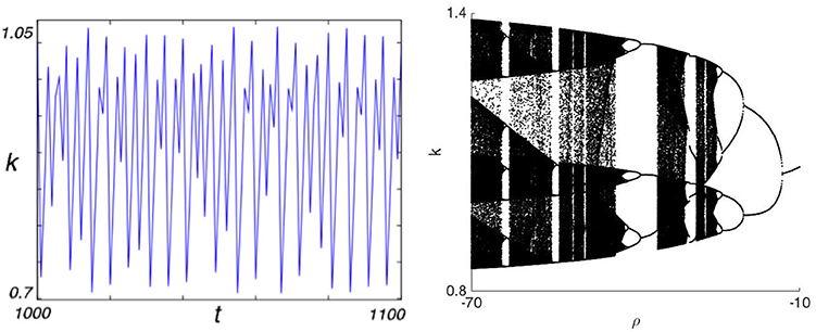
Figure 2. (Left) Time-line of BK model with f_c production function for ρ < 0 and s_r>s_w. (Right) Bifurcation diagram w.t.r. ρ (parameter related to the elasticity of substitution).

Remark 3.2. Consider the Leontief production function as defined in Equation (12). Then the BK model (Equation 6) may generate complex dynamics iff

$s_r>s_w\wedge s_r>\frac{n+\delta }{a}.$

(For proof see [15])

From Remarks 3.1 and 3.2 it emerges that, when a production function with constant elasticity of substitution is considered in the BK model, fluctuations may emerge in the economy only if the ES is lower than one and the saving propensity of shareholders is higher than that of workers. In the following we report conditions on parameters for cyclical and chaotic behaviors when considering technologies belonging to the class of VES production functions.

3.2. BK Model With VES Production Function

The interest on VES production functions is driven by the results of empirical studies (see [16, 17]) that prove the validity of this technology in representing reality. Recall that with VES production functions the ES moves depending on changes in the economy's per capita capital level (for a detailed analysis of the influence of ES on growth see [18]).

3.2.1. Revankar Production Function

In order to analyse how the VES technology influences long run behavior of an economy we report the results obtained by Brianzoni et al. [19] considering the Revankar production function

$\begin{array}{cc}\begin{array}{r}{f}_r(k_t):=A{k}_t^{\alpha }{(1+\alpha \beta k_t)}^{1-\alpha }\end{array}& (13)\end{array}$

where A > 0 measures the technological progress while α ∈ (0, 1) and $\beta \ge -\frac{1}{k}$ refer to the output elasticity of inputs. Notice that the production function does not verify one of the weak Inada conditions, i.e., $\underset{k_t\to \infty }{lim}\frac{f_r(k_t)}{k_t}\ne 0$. Following the definition given in Sato and Hoffman [8], the ES of the Revankar technology is the linear function

$\begin{array}{cc}\begin{array}{r}\sigma (k_t)=1+\beta k_t\end{array}& (14)\end{array}$

and it varies depending on k_t. As for the CES production function, when σ > 1 only simple dynamics may arise and the saving propensity of shareholders influences them: a stable long run equilibrium exists when s_r is sufficiently small, and unbounded growth is observed otherwise. When the ES falls below one, up to three attractors may exist and fluctuation arises when the ES decreases. Necessary conditions on parameters for chaotic behaviors to emerge are summarized in the following Remark.

Remark 3.3. Consider the Revankar production function as defined in Equation (13). Then the BK model (Equation 6) may generate complex dynamics iff

$s_r\ge s_w\wedge b\in [-1,0).$

(For proof see [19])

Notice that condition b ∈ [−1, 0) implies σ < 1, so complex behavior may arise only when the ES is smaller than one.

3.2.2. Sigmoidal Production Function

Revankar technology satisfies $\underset{k_t\to 0}{lim}{f}_r^{\prime }(k_t)=+\infty$, that is, infinitely high returns may be reached with a small investment on capital when no physical capital exist. This hypothesis is unrealistic since, for production, a previous investment on infrastructures, machineries, as well as know-how is needed. Driven by this consideration, Brianzoni et al. [20] studies the BK model with the sigmoidal production function

$\begin{array}{cc}\begin{array}{r}{f}_s(k_t):=\frac{\alpha k_t^{\rho }}{1+\beta k_t^{\rho }}\end{array}& (15)\end{array}$

with α and β positive and ρ ≥ 2. The ES for the f_s technology is given by

$\begin{array}{cc}\begin{array}{r}\sigma (k_t)=\frac{\beta \rho k_t^{\rho }}{\rho (1-\beta k_t^{\rho })-(1+\beta k_t^{\rho })}+1\end{array}& (16)\end{array}$

and it depends on k_t, so the f_s technology belongs to the class of VES production functions. Moreover, this technology does not verify the weak Inada conditions. In this case a fixed point characterized by zero capital per capita exists and hence the considered production function it is able to explain the poverty trap effect. Furthermore, the authors found that a sufficiently low ES is needed for cycles or chaos to be observed. Necessary conditions for fluctuations to emerge are summarized in the following Remark.

Remark 3.4. Consider the sigmoidal production function as defined in Equation (15). Then a $\bar{\rho }>0$ exists such that the BK model (Equation 6) may generate complex dynamics iff

$s_r>s_w\wedge \rho >\bar{\rho }.$

(For proof see [20])

Notice that the elasticity of substitution decreases as ρ increases, so complex behavior may arise only when the ES is sufficiently low, i.e., $\sigma <\bar{\sigma }$, where $\bar{\sigma }$ is the elasticity of substitution for $\rho =\bar{\rho }$.

3.2.3. Shifted Cobb-Douglas Production Function

Although the sigmoidal production function f_s does not allow infinitely high returns, it still admits production when the capital per capita approaches zero. Grassetti et al. [21] argues that a minimum level of capital is needed before making returns and proposed the Shifted Cobb-Douglas (SCD) production function, compared to the sigmoidal in Figure 3.

FIGURE 3

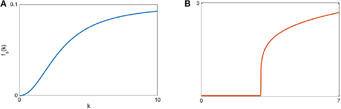
Figure 3. (A) Sigmoidal production function. (B) Shifted Cobb-Douglas production function.

The SCD technology is given by

$\begin{array}{cc}{f}_{SCD}(k_t)=\{\begin{array}{c}\begin{array}{cc}0& 0\le k_t\le k_c\\ A{(k_t-k_c)}^{\alpha }& k_t>k_c\end{array}\end{array}& (17)\end{array}$

where A > 0 is the total productivity factor, 0 < α < 1 is the output elasticity of capital and k_c ≥ 0 the minimum capital per capita initial level needed for production. In this case the ES is

$\sigma (k_t)=\{\begin{array}{l}\begin{array}{cc}+\infty & 0<k_t<k_c\\ 1-\frac{k_c}{(1-\alpha )k_t}& k_t>k_c\end{array}.\hfill \end{array}$

Notice that σ is always smaller than one when output is positive, and it varies depending on the level of capital per capita. When the SCD function is considered, fluctuations may always emerge (notice that σ < 1 ∀k_t > k_c) and, once again, multistability phenomena exist when shareholders save more than workers. Distinct from all previous cases, up to three attractors may exist.

3.2.4. Kadyiala Production Function

VES production functions considered in previous works show monotone elasticity of substitution between capital and labor. Kadyiala [22] noted that σ should increase (decrease) as the input ratio k tends to a critical value and decrease (increase) thereafter, making the ES symmetric for capital and labor. The author suggested a new production function to fix this issue. The [22] technology is given by

$\begin{array}{cc}\begin{array}{r}{f}_k(k_t):=A{(a{k}_t^{2\rho }+2b{k}_t^{\rho }+c)}^{12\rho }\end{array}& (18)\end{array}$

where a, b and c are non-negative with a + 2b + c = 1, A < 0 and $\rho \le \frac{1}{2}$, ρ ≠ 0. For this production function the ES is given by

$\begin{array}{cc}\begin{array}{r}\sigma (k_t)=\frac{1}{1-\rho +R},\end{array}& (19)\end{array}$

where $R=\frac{-\rho (ac-b^2)}{(a{k}_t^{-\rho }+b)(b+c{k}_t^{\rho })}$. Notice that σ ≥ 1 if and only if ρ > 0. When the Kadyiala technology is considered, fluctuations and chaotic dynamics may emerge depending on parameters values, as summarized in the following Remark.

Remark 3.5. Consider the Kadyiala production function as defined in Equation (18). Then the BK model (Equation 6) may generate complex dynamics iff

$\frac{n+\delta }{A{a}^{\frac{1}{2\rho }}}>s_r>s_w\wedge \rho <0.$

(For proof see [23])

Notice that ρ > 0 implies σ < 1, so once again fluctuations may arise if and only if the elasticity of substitution is lower than one, and the saving behavior of shareholders influences the evolution of capital: boom and bust periods may arise only if shareholders do not invest enough. Finally the authors find that multistability phenomena may emerge when the elasticity of substitution between production factors is lower than one.

4. Factors Determining Growth Equilibria and Fluctuations

In the previous sections we analyzed the role played by technologies and by the saving propensities of workers and shareholders (respectively s_w and s_r) on the evolution of capital per capita, when the BK model ([1]) is considered. The main findings of each contribution on the existence of fixed points for the economy are summarized in Table 1.

TABLE 1

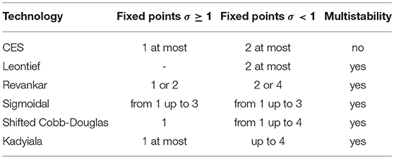
Table 1. steady states and multistability phenomena in BK model.

We recall that the saving propensity of workers influences the lower bound that the economy may reach during boom and bust periods (the higher s_w, the higher the level of capital per capita in bust periods),and that an increment on s_w would increase the upper bound of growth for developed economies while decreasing that of non developed economies. Conversely, the saving behavior of shareholders influences the maximum feasible growth (the higher s_r, the higher the upper bound of capital per capita). It is worthwhile to highlight that only the saving propensity of shareholders influences the existence and stability of equilibria: when the ES is higher than one, regardless of the considered technology, unbounded growth is possible when shareholders invest enough. Moreover, when shareholders save more than workers multiple attractors emerge. Concerning the influence of elasticity of substitution on growth, it has been found that regardless of the considered technology, the ES determines both existence and stability of equilibria: only for σ < 1 multistability phenomena may exist (and hence the model is able to describe the evolution of different economies over time) and fluctuation may arise. It is worth highlighting that changes in the considered technology affect the existence of poverty trap and the number of equilibria, but they do not entail new conditions on cycles and more complex dynamics emerging. Necessary conditions on s_r, s_w and σ for fluctuations, for the analyzed technologies are summarized in Table 2.

TABLE 2

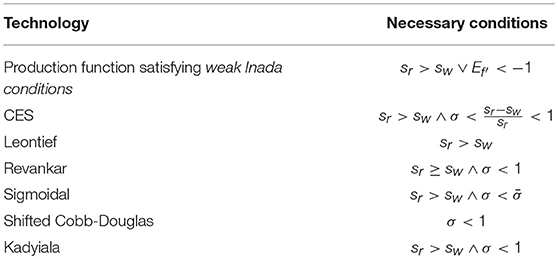
Table 2. necessary conditions for complex dynamics.

For all the considered technologies, regardless of the fulfillment of weak Inada conditions, complex behaviors may emerge only when the elasticity of substitution is sufficiently low. Notice that when workers save more than shareholders only simple dynamics are possible, except for the case in which the Shifted Cobb-Douglas production function is considered. Moreover, the saving behavior of shareholders influences the long run evolution of an economy described by the BK model. Even though similar conditions are given for all the production functions, it is interesting to analyse how the evolution over time differs, when different technologies are considered. To this aim, in Figure 4 we show the bifurcation diagram for the BK model when considering the cited technologies.

FIGURE 4

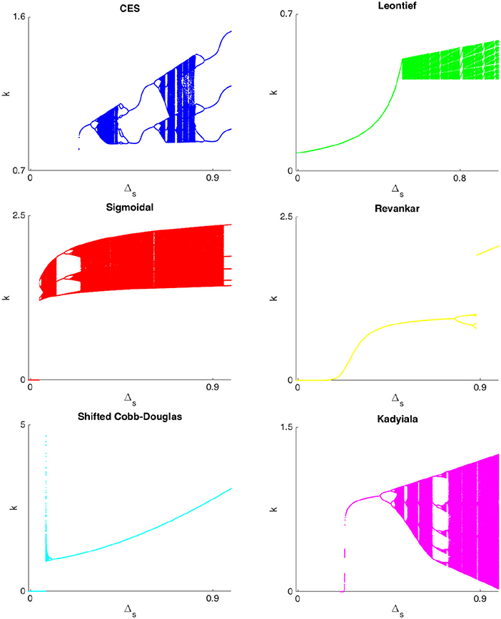
Figure 4. Bifurcation diagram w.r.t. Δ_s for BK model considering CES (blue), Leontief (green), sigmoidal (red), Revankar (yellow), SCD (cyan), and Kadyiala (magenta) technologies.

We assume Δ_s = s_r−s_w and, for all the production functions, we fix the same values of the depreciation rate of capital (δ = 0.1), the labor force growth rate (n = 0.15), the saving behavior of workers (s_w = 0.01), the total productivity factor (A = 1) and the output elasticity of capital (a = α = 0.4). We then analyse the bifurcation diagram for all the maps starting from the initial condition k₀ = 1. Recall that when the CES (Equation 11), the sigmoidal (Equation 15) or the Kadyiala (Equation 18) production functions are considered in the BK model given by Equation (6), the final model is a continuous and smooth map, while it is piecewise-smooth when considering the SCD (Equation 17) or the Revankar (Equation 13) (only for b ∈ [−1, 0), see [19]) production functions. Lastly, the final map is piecewise-linear when adopting the Leontief technology given in Equation (12). In blue is shown the bifurcation diagram for the CES production function: period doubling and period halving bifurcations (for period halving bifurcations see [13]) emerge as the difference between saving behaviors increases, and chaotic dynamics exist. A period doubling route to chaos (without period halving bifurcations) is clearly visible also with sigmoidal production function (red line) as well as for the Kadyiala one (magenta line). This is in contrast with the Revankar technology (yellow line), where a border collision bifurcation (BCB) interrupts a sequence of flip bifurcations (for BCB in economic models see [24–26]) when Δ_s is sufficiently high. When considering the SCD technology (cyan line), a BCB terminates the poverty trap and a complex attractor immediately thereafter. The bifurcation diagram for Leontief technology is depicted in green: a sequence of BCBs occurs and cycles of different orders emerge. It is worthwhile noting that complex dynamics emerge when the difference between the saving rates of the two income group are sufficiently high, and the poverty trap phenomenon is always seen for VES production functions when workers and shareholders have a similar saving behavior.

5. Conclusions

In this review on growth theory we analyse the influence of technologies and saving propensities of workers and shareholders on economic growth, considering the BK model. Our objective was to show how investing behaviors and production peculiarities condition the evolution of capital over time. We focused on the existence of multistability phenomena that would explain why GDP increases over time in developed economies while being mainly stagnant in developing countries. We found that both fluctuations and multiple equilibria may arise only when the elasticity of substitution is lower than one. Savings behaviors of workers and shareholders influence stability of equilibria while only VES production functions are able to describe the poverty trap without any restriction on other conditions. It has been shown that, regardless of the considered technology, complex dynamics emerge when the difference between the saving propensity of workers and shareholders is sufficiently high while a poverty trap may exist when the two income groups have similar saving behaviors.

Author Contributions

The author confirms being the sole contributor of this work and has approved it for publication.

Conflict of Interest Statement

The author declares that the research was conducted in the absence of any commercial or financial relationships that could be construed as a potential conflict of interest.

The Reviewer JDO is the Senior Managing Director, Chief Analytics Officer at DataMineit, LLC.

Footnotes

1. ^See [9] for results with no restrictions on parameter values.

2. ^Notice that neoclassical growth theory considers production functions that satisfy Constant Returns to Scale (CRS), i.e., F(μK_t, μL_t) = μF(K_t, L_t), ∀ μ > 0. Moreover, it assumes positive and diminishing marginal products of capital and labor so that $\frac{\partial F(K_t,L_t)}{\partial K_t}>0$, $\frac{{\partial }^{2}F(K_t,L_t)}{\partial K_t^2}<0$, $\frac{\partial F(K_t,L_t)}{\partial L_t}>0$, $\frac{{\partial }^{2}F(K_t,L_t)}{\partial L_t^2}<0$ and it requires fulfillment of the Inada conditions (see [10]) given by

$\begin{array}{l}{\lim }_{K_t\to \infty }\frac{\partial F(K_t,L_t)}{\partial K_t}={\lim }_{L_t\to \infty }\frac{\partial F(K_t,L_t)}{\partial L_t}=0,\\ {\lim }_{K_t\to 0}\frac{\partial F(K_t,L_t)}{\partial K_t}={\lim }_{L_t\to 0}\frac{\partial F(K_t,L_t)}{\partial L_t}=\infty ,\end{array}$

Notice that Inada conditions imply positive and decreasing marginal returns of inputs. An example of technology verifying the previous conditions is the Cobb-Douglas (CD) production function, which can be written in intensive form as $f_{cd}(k_t):=k_t^{\alpha }$, where α ∈ (0, 1) is the output elasticity of capital. This technology is characterized by constant elasticity of substitution equal to one, i.e., σ = 1. When the CD production function is considered in Equation (6), almost all initial conditions produce trajectories that monotonically converge to the unique positive fixed point and no fluctuations may be generated.

3. ^The case in which an initial condition k₀ > 0 generates a trajectory converging to the equilibria characterized by 0 capital per capita.

References

1. Böhm V, Kaas L. Differential savings, factor shares, and endogenous growth cycles. J Econ Dyn Control. (2000) 24:965–80. doi: 10.1016/S0165-1889(99)00032-9

CrossRef Full Text | Google Scholar

2. Solow RM. A contribution to the theory of economic growth. Q J Econ. (1956) 70:65–94.

Google Scholar

3. Harrod RF. An essay in dynamic theory. Econ J. (1939) 49:14–33.

Google Scholar

4. Domar ED. Capital expansion, rate of growth, and employment. Econometrica (1946)14:137–47.

Google Scholar

5. Kaldor N. Marginal productivity and the macro-economic theories of distribution: comment on marginal productivity and the macro-economic theories of distribution: comment on samuelson and modigliani. Rev Econ Stud. (1966) 33:309–19.

Google Scholar

6. Kaldor N. A model of economic growth. Econ J. (1957) 67:591–624.

Google Scholar

7. Kaldor N. Alternative theories of distribution. Rev Econ Stud. (1956) 23:83–100.

Google Scholar

8. Sato R, Hoffman RF. Production functions with variable elasticity of factor substitution: Some analysis and testing. Rev Econ Stat. (1968) 50:453–60.

Google Scholar

9. Grassetti F, Hunanyan G, Mammana C, Michetti E. A note on the influence of saving behaviors on economic growth. Metroeconomica (2018). doi: 10.1111/meca.12210. [Epub ahead of print].

CrossRef Full Text | Google Scholar

10. Inada K. On a two-sector model of economic growth: comments and a generalization. Rev Econ Stud. (1963) 30:119–27.

Google Scholar

11. Brianzoni S, Mammana C, Michetti E. Complex dynamics in the neoclassical growth model with differential savings and non-constant labor force growth. Stud Nonlinear Dyn Econometr. (2007) 11:3. doi: 10.2202/1558-3708.1407

CrossRef Full Text | Google Scholar

12. Brianzoni S, Mammana C, Michetti E. Nonlinear dynamics in a business-cycle model with logistic population growth. Chaos Solitons Fractals (2009) 40:717–30. doi: 10.1016/j.chaos.2007.08.041

CrossRef Full Text | Google Scholar

13. Hommes C. Dynamics of the cobweb model with adaptive expectations and nonlinear supply and demand. J Econ Behav Organ. (1994) 24:315–35.

Google Scholar

14. Allen RGD. Mathematical Economics. London: Macmillan (1956).

Google Scholar

15. Tramontana F, Gardini L, Agliari A. Endogenous cycles in discontinuous growth models. Math Comput Simul. (2011) 81:1625–39. doi: 10.1016/j.matcom.2010.12.002

CrossRef Full Text | Google Scholar

16. Bairam E. Capital-labor substitution and slowdown in soviet economic growth: a Re-examination. Bull Econ Res. (1990) 42:63–72.

Google Scholar

17. Karagiannis G, Palivos T, Papageorgiou C. Variable elasticity of substitution and economic growth.In: Diebolt C, Kyrtsou C (editors). New Trends in Macroeconomics (2005). p. 21–37.

Google Scholar

18. Grassetti F, Mammana C, Michetti E. Substitutability between production factors and growth. An analysis using VES production functions. Chaos Solitons Fractals (2018) 113:53–62. doi: 10.1016/j.chaos.2018.04.012

CrossRef Full Text | Google Scholar

19. Brianzoni S, Mammana C, Michetti E. Variable elasticity of substitution in a discrete time Solow-Swan growth model with differential saving. Chaos Solitons Fractals (2012) 45:98–108. doi: 10.1016/j.chaos.2011.10.004

CrossRef Full Text | Google Scholar

20. Brianzoni S, Mammana C, Michetti E. Local and global dynamics in a discrete time growth model with nonconcave production function. Discrete Dyn Nat Soc. (2012) 2012:1–22. doi: 10.1155/2012/536570

CrossRef Full Text | Google Scholar

21. Grassetti F, Mammana C, Michetti E. Poverty trap, boom and bust periods and growth. A non-linear model for non-developed and developing countries. Decisions Econ Finan. (2018) 41:145. doi: 10.1007/s10203-018-0211-6

CrossRef Full Text | Google Scholar

22. Kadyiala KR. Production functions and elasticity of substitution. South Econ J. (1972) 38:281–4.

Google Scholar

23. Grassetti F, Hunanyan G. On the economic growth theory with kadiyala production function. Commun Nonlinear Sci Numerical Simul. (2018) 58:220–32. doi: 10.1016/j.cnsns.2017.06.036

CrossRef Full Text | Google Scholar

24. Tramontana F, Gardini L, Puu T. Duopoly games with alternative technologies. J Econ Dyn Control. (2009) 33:250–65. doi: 10.1016/j.jedc.2008.06.001

CrossRef Full Text | Google Scholar

25. Puu T, Sushko I. Business Cycle Dynamics, Models and Tools. Berlin: Springer Verlag (2006).

Google Scholar

26. Puu T, Sushko I. Oligopoly Dynamics Models and Tools. Berlin: Springer Verlag (2002).

Google Scholar