Data Based Construction of Kernels for Semi-Supervised Learning With Less Labels

This paper deals with the problem of semi-supervised learning using a small number of training samples. Traditional kernel based methods utilize either a fixed kernel or a combination of judiciously chosen kernels from a fixed dictionary. In contrast, we construct a data-dependent kernel utilizing the Mercer components of different kernels constructed using ideas from diffusion geometry, and use a regularization technique with this kernel with adaptively chosen parameters. Our algorithm is illustrated using a few well-known data sets as well as a data set for automatic gender identification. For some of these data sets, we obtain a zero test error using only a minimal number of training samples.

1. Introduction

The problem of learning from labeled and unlabeled data (semi-supervised learning) has attracted considerable attention in recent years. A variety of machine learning algorithms use Tikhonov single penalty or multiple penalty schemes for regularizing with different approaches to data analysis. Many of these are kernel based algorithms that provide regularization in Reproducing Kernel Hilbert Spaces (RKHS). The problem of finding a suitable kernel for learning a real-valued function by regularization is considered, in particular, in the papers [1–3] (see also the references therein), where different approaches were proposed. All the methods mentioned in these papers deal with some set of kernels that appear as a result of parametrization of classical kernels, a kind of convolution of “inner” and “outer” kernels, or linear combination of some functions. Such approaches lead to the problem of multiple kernel learning. In this way, the kernel choice problem is somehow shifted to the problem of a description of a set (a dictionary of kernels), on which a multiple kernel learning is performed.

In the present paper we propose an approach to construct a kernel directly from observed data rather than combining kernels from a given dictionary. The approach uses ideas from diffusion geometry [see, e.g., [4–8]], where the eigenvectors of the graph Laplacian associated to the unlabeled data are used to mimic the geometry of the underlying manifold that is usually unknown. The literature on this subject is too large to be cited extensively. The special issue [9] of “Applied and Computational Harmonic Analysis” is devoted to an early review of this subject. Most relevant to the current paper are the papers [7, 10], where the graph Laplacian associated to the data has been used to form additional penalty terms in a multi-parameter regularization functional of Tikhonov type. In contrast to Belkin et al. [7] and Bertozzi et al. [10], we use eigenvectors and eigenfunctions of the corresponding family of graph Laplacians (rather than a combination of these graph Laplacians) to construct a data-dependent kernel that directly generates an RKHS.

The paper is organized as follows: in the next two sections we present the main theoretical background. Then, we give the numerical algorithms for the implementation of the proposed method. Finally, we provide experimental results with their discussion.

2. Background

The subject of diffusion geometry seeks to understand the geometry of the data ${\left\{x_i\right\}}_{i=1}^n\subset {ℝ}^D$ drawn randomly from an unknown probability distribution μ, where D is typically a large ambient dimension. It is assumed that the support of μ is a smooth sub-manifold of ℝ^D having a small manifold dimension d. It is shown in Jones et al. [11] that a local coordinate chart of the manifold can be described in terms of the values of the heat kernel, respectively, those of some of the eigenfunctions, of the so called Laplace-Beltrami operator on the unknown manifold. However, since the manifold is unknown, one needs to approximate the Laplace-Beltrami operator. One way to do this is using a graph Laplacian as follows.

For ϵ > 0 and x, y ∈ ℝ^D, let:

$\begin{array}{ll}{W}^{\epsilon }(x,y):=exp\left(-\frac{\left|\right|x-y|{|}^2}{4\epsilon }\right).& (1)\end{array}$

We consider the points ${\left\{x_i\right\}}_{i=1}^n$ as vertices of an undirected graph with the edge weight between x_i and x_j given by $W^{\epsilon }(x_i,x_j)$, thereby defining a weighted adjacency matrix, denoted by W^ε. We define D^ε to be the diagonal matrix with the i-th entry on the diagonal given by ${\displaystyle \sum _{j=1}^n{W}^{\epsilon }}(x_i,x_j)$. The graph Laplacian is defined by the matrix:

$\begin{array}{ll}{\text{L}}^{\epsilon }=\frac{1}{n}\left\{{\text{D}}^{\epsilon }-{\text{W}}^{\epsilon }\right\}.& (2)\end{array}$

We note that for any real numbers a₁, ⋯ , a_n,

${\displaystyle \sum _{i,j=1}^n}{a}_i{a}_j{L}_{i,j}^{\epsilon }=\frac{1}{2n}{\displaystyle \sum _{i,j=1}^n}{W}_{i,j}^{\epsilon }{(a_i-a_j)}^2.$

We conclude that the eigenvalues of L^ε are all real and non-negative, and therefore, can be ordered as:

$\begin{array}{ll}0={\lambda }_1^{\epsilon }\le {\lambda }_2^{\epsilon }\le \cdots \le {\lambda }_n^{\epsilon }.& (3)\end{array}$

It is convenient to consider the eigenvector corresponding to ${\lambda }_k^{\epsilon }$ to be a function on ${\left\{x_j\right\}}_{j=1}^n$ rather than a vector in ℝⁿ, and denote it by ${\varphi }_k^{\epsilon }$, thus:

$\begin{array}{l}{\lambda }_k^{\epsilon }{\varphi }_k^{\epsilon }(x_i)={\displaystyle \sum _{j=1}^n{L}_{i,j}^{\epsilon }}{\varphi }_k^{\epsilon }(x_j)=\frac{1}{n}({\varphi }_k^{\epsilon }(x_i){\displaystyle \sum _{j=1}^n{W}^{\epsilon }}(x_i,x_j)\\ -{\displaystyle \sum _{j=1}^n{W}^{\epsilon }}(x_i,x_j){\varphi }_k^{\epsilon }(x_j)),\\ i=1,\dots ,n.& (4)\end{array}$

Since the function W^ε is defined on the entire ambient space, one can extend the function ${\varphi }_k^{\epsilon }$ to the entire ambient space using (4) in an obvious way (the Nyström extension). Denoting this extended function by ${\Phi }_k^{\epsilon }$, we have:

$\begin{array}{l}{\lambda }_k^{\epsilon }{\text{Φ}}_k^{\epsilon }(x)=\frac{1}{n}\left({\text{Φ}}_k^{\epsilon }(x){\displaystyle \sum _{j=1}^n}{W}^{\epsilon }(x,x_j)-{\displaystyle \sum _{j=1}^n}{W}^{\epsilon }(x,x_j){\varphi }_k^{\epsilon }(x_j)\right),\\ x\in {ℝ}^D.& (5)\end{array}$

More explicitly, [cf. von Luxburg et al. [12]]

$\begin{array}{ll}{\text{Φ}}_k^{\epsilon }(x)=\frac{{\displaystyle {\sum }_{j=1}^n}{W}^{\epsilon }(x,x_j){\varphi }_k^{\epsilon }(x_j)}{{\displaystyle {\sum }_{j=1}^n}{W}^{\epsilon }(x,x_j)-n{\lambda }_k^{\epsilon }},& (6)\end{array}$

for all x ∈ ℝ^D for which the denominator is not equal to 0. The condition that the denominator of (6) is not equal to 0 for any x can be verified easily for any given ε. The violation of this condition for a particular k can be seen as a sign that for given amount n of data the approximations of the eigenvalue λ_k of the corresponding Laplace-Beltrami operator by eigenvalues ${\lambda }_k^{\epsilon }$ cannot be guaranteed with a reasonable accuracy.

We end this section with a theorem [13, Theorem 2.1] regarding the convergence of the extended eigenfunctions ${\Phi }_k^{\epsilon }$, restricted to a smooth manifold X, to the actual eigenfunctions of the Laplace-Beltrami operator on X. We note that each ${\Phi }_k^{\epsilon }$ is constructed from a randomly chosen data ${\left\{x_i\right\}}_{i=1}^n$ from some unknown manifold X, and is therefore, itself a random variable.

Theorem 1. Let X be a smooth, compact manifold with dimension d, and μ be the Riemannian volume measure on X, normalized to be a probability measure. Let ${\left\{x_i\right\}}_{i=1}^n$ be chosen randomly from μ, ${\Phi }_k^{\epsilon }$ be as in (6), and Φ_k be the eigenfunction of the Laplace-Beltrami operator on X that has the same ordering number as k, corresponding to the eigenvalue λ_k. Then there exists a sequence ε_n → 0, such that:

$\begin{array}{ll}{\displaystyle \underset{n\to \infty }{lim}}\frac{1}{{\epsilon }^{1+d/2}}|{\lambda }_k^{{\epsilon }_n}-{\lambda }_k|=0,& (7)\end{array}$

and

$\begin{array}{ll}{\displaystyle \underset{n\to \infty }{lim}}||{\text{Φ}}_k^{{\epsilon }_n}-{\text{Φ}}_k||=0,& (8)\end{array}$

where the norm is the L² norm, and the limits are taken in probability generated by μ.

3. Numerical Algorithms for Semi-Supervised Learning

The approximation theory utilizing the eigen-decomposition of the Laplace-Beltrami operator is well developed, even in greater generality than this setting, in Maggioni and Mhaskar [14], Filbir and Mhaskar [15], Mhaskar [16], Mhaskar [17], and Ehler et al. [18]. In practice, the correct choice of ε in the approximate construction of these eigenvalues and eigenfunctions is a delicate matter that affects greatly the performance of the kernel based methods based on these quantities. Some heuristic rules for choosing ε have been proposed in Lafon [8] and Coifman and Hirn [19]. These rules are not applicable universally; they need to be chosen according to the data set and the application under consideration.

In contrast to the traditional literature, where a fixed value of ε is used for all the eigenvalues and eigenfunctions, we propose in this paper the construction of a kernel of the form:

$\begin{array}{ll}{K}_n(x,t)={\displaystyle \sum _k}{(n{\lambda }_k^{{\epsilon }_{j_k}})}^{-1}{\text{Φ}}_k^{{\epsilon }_{j_k}}(x){\text{Φ}}_k^{{\epsilon }_{j_k}}(t);& (9)\end{array}$

That is, we select the eigenvalues and the corresponding eigenfunctions from different kernels of the form W^ε to construct our kernel. We note again that in contrast to the traditional method of combining different kernels from a fixed dictionary, we are constructing a single kernel using the Mercer components of different kernels from a dictionary.

Our rule for the selection of the parameter ε_jk's is based on the well-known quasi-optimality criterion [20] that is one of the simplest and oldest, but still a quite efficient strategy for choosing a regularization parameter. According to that strategy, one selects a suitable value of ε (i.e., regularization parameter) from a sequence of admissible values {ε_j}, which usually form a geometric sequence, i.e., ${\epsilon }_j={\epsilon }_0{q}^j,j=1,2,\dots ,M;q<1$. We propose to employ the quasi-optimality criterion in the context of the approximation of the eigenvalues of the Laplace-Beltrami operator. Then by analogy to Tikhonov and Glasko [20] for each particular k we calculate the sequence of approximate eigenvalues ${\lambda }_k^{{\epsilon }_j},j=1,2,\dots ,M$, and select ε_jk ∈ {ε_j} such that the differences $|{\lambda }_k^{{\epsilon }_j}-{\lambda }_k^{{\epsilon }_{j-1}}|$ attain their minimal value at j = j_k.

Since the size of the grid of ε_j is difficult to be estimated beforehand and, at the same time, has a strong influence on the performance of the method, we propose the following strategy for the selection of the grid size M. We note that the summation in formula (9) has to be done for indices k for which the corresponding eigenvalue ${\lambda }_k={\lambda }_k^{{\epsilon }_{j_k}}$ is non-zero. It is also known that the first eigenvalue ${\lambda }_1^{{\epsilon }_j}=0$. To prevent the other ${\lambda }_k^{{\epsilon }_j}$ from becoming too close to zero with the decreasing of ε_j, we propose to stop continuation of the sequence ε_j as soon as the value of ${\lambda }_2^{{\epsilon }_M}$ becomes sufficiently small. So, the maximum grid size M is the smallest integer for which ${\lambda }_2^{{\epsilon }_M}<{\lambda }_2^{(thr)}$, where ${\lambda }_2^{(thr)}$ is some estimated threshold. Taking the abovementioned into account, we also replace the formula for the kernel calculation (9) by the kernel:

$\begin{array}{ll}{K}_n(x,t)=1+{\displaystyle \sum _{k=2}^n}{(n{\lambda }_k^{{\epsilon }_{j_k}})}^{-1}{\text{Φ}}_k^{{\epsilon }_{j_k}}(x){\text{Φ}}_k^{{\epsilon }_{j_k}}(t);& (10)\end{array}$

The Algorithm 1 below describes the combination of the approximation (6) with quasi-optimality criterion.

ALGORITHM 1

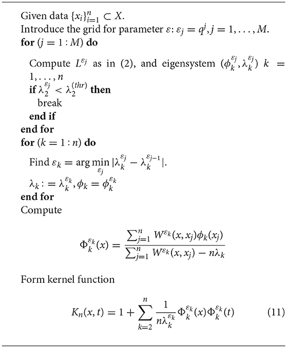
Algorithm 1: Algorithm to generate reproducing kernel from data

Algorithm 2 uses the constructed kernel (11) in kernel ridge regression from labeled data. The regression is performed in combination with discrepancy based principle for choosing the regularization parameter α.

ALGORITHM 2

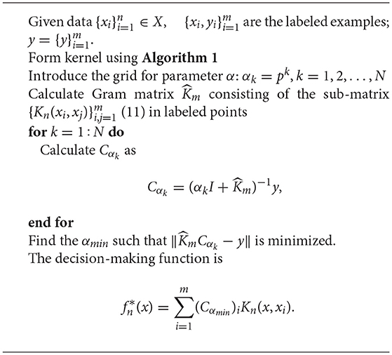
Algorithm 2: Algorithm for kernel ridge regression with the constructed kernel (11)

4. Experimental Results

4.1. Two Moons Dataset

In this section we consider classification of the two moons dataset that can be seen as the case D = 2, d = 1. The software and data were borrowed from bit.ly/2D3uUCk. For the two moons dataset we take ${\left\{x_i\right\}}_{i=1}^n$ with n = 50, 30, 10 and subsets ${\left\{x_i\right\}}_{i=1}^m\subset {\left\{x_i\right\}}_{i=1}^n$ with m = 2, 4, 6 labeled points. The goal of semi-supervised data classification problems is to assign correct labels for the remaining points ${\left\{x_i\right\}}_{i=1}^n\backslash {\left\{x_i\right\}}_{i=1}^m$. For every dataset (defined by the pair (n, m)) we performed 10 trials with randomly chosen labeled examples.

As follows from the experiments, the accuracy of the classification is improving with the growth of the number of unlabeled points. In particular, for n = 50, to label all points without error, it is enough to take only one labeled point for each of two classes (m = 2). At the same time, if the set of unlabeled points is not big enough, then for increasing the accuracy of prediction we should take more labeled points. The result of the classification for the two moons dataset with m = 2 as well as the corresponding plot of selected ε are shown in Figures 1, 2. The big crosses correspond to the labeled data and other points are colored according to the constructed predictors. The parameters' values were m=2, ϵ₀ = 1, q=0.9, ${\lambda }_2^{(thr)}=10^{-6}$.

FIGURE 1

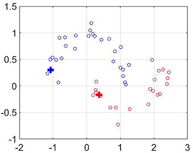
Figure 1. Classification of “two moons” dataset with extrapolation region. The values of parameters are m=2, ϵ₀ = 1, q=0.9, ${\lambda }_2^{(thr)}=10^{-6}$.

FIGURE 2

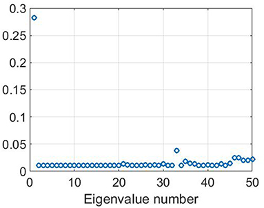
Figure 2. Plot of adaptively chosen ε for two-moon dataset. The values of parameters are m=2, ϵ₀ = 1, q=0.9, ${\lambda }_2^{(thr)}=10^{-6}$.

Note that “two moons” dataset from Figure 1 has been also used for testing the performance of a manifold learning algorithm realized as a multi-parameter regularization [21]. The comparison of Table 1 with Table 6 of Lu and Pereverzyev [21] shows that on the dataset from Figure 1 the Algorithms 1–2 based on the kernel (11) outperform the algorithm from Lu and Pereverzyev [21], where the graph Laplacian has been used as the second penalization operator, and much more unlabeled points have been involved in the construction of the classifiers. For example, to achieve zero classification error on the dataset from Figure 1 the algorithm [21] needs to know at least 10 labeled and 190 unlabeled points, while the Algorithms 1–2 allow perfect classification using only 2 labeled and 50 unlabeled points.

TABLE 1

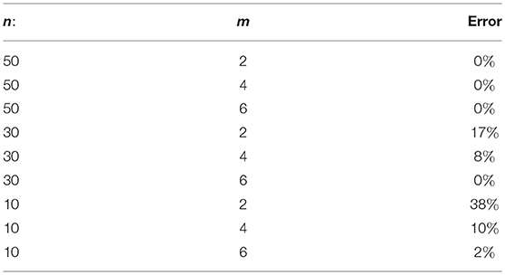
Table 1. Results of testing for two moons dataset.

In our next experiment, we follow [10] and embed the two moons dataset in ℝ¹⁰⁰ by adding 98-dimensional zero-mean Gaussian random vectors with standard deviation σ. Then the Algorithms 1–2 have been applied to the transformed data set, which means that in (1) the symbol ||·|| is staying for ℝ¹⁰⁰-norm. The results of the experiment with only two labeled points, m = 2, are presented in Table 2. The performance displayed in this table is comparable to the one reported in Bertozzi et al. [10], but the above performance has been achieved with minimal admissible number of labeled points, i.e., m = 2, while in Bertozzi et al. [10] the tests have been performed with n = 2000, m = 60. Note that according to Theorem 1 the use of large number n of unlabeled points allows better approximation of the eigenvalues and eigenfunctions of the corresponding Laplace-Beltrami operators and may potentially improve the performance of the Algorithms 1–2. At the same time, the realization of these algorithms for large number n, such as n = 2000, may become more computationally intensive as compared to Bertozzi et al. [10]. Therefore, a comparison of our results with those in Bertozzi et al. [10] is not so straightforward.

TABLE 2

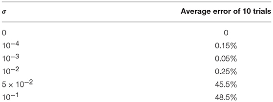
Table 2. Results of testing for two moons dataset embedded in ℝ¹⁰⁰, n = 200, m = 2.

4.2. Two Circles Datasets

In this section, we consider two “two-circles” datasets. Each circle has unit radius and contains 100 points so that n = 200. These datasets are depicted at Figures 3, 4, respectively.

FIGURE 3

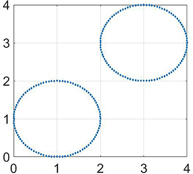
Figure 3. Testing dataset of two non-intersecting circles.

FIGURE 4

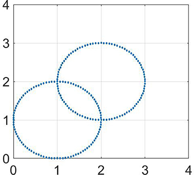
Figure 4. Testing dataset of two intersecting circles.

Below we consider classification of these datasets by the proposed method. As can be seen from Figure 5, for non-intersecting circles only m = 2 labeled points are enough for a correct classification of the given set.

FIGURE 5

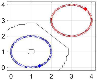
Figure 5. Classification of “two non-intersecting circles” dataset. The values of parameters are n = 200, m = 2, M = 70, p = 0.5, q = 0.9.

Figure 6 shows the classification results for m = 20 labeled points at the intersected circles. The big crosses correspond to the labeled data and other points are colored according to the constructed predictors. The error percentage for different m is shown in Table 3. It can be seen that the classification error decreases with the growth of the number m of labeled points. The fact that not all points are correctly classified can be explained by the non-smoothness of the considered manifold.

FIGURE 6

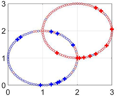
Figure 6. Classification of “two intersecting circles” dataset. The values of parameters are n = 200, m = 20, M = 70, p = 0.5, q = 0.9.

TABLE 3

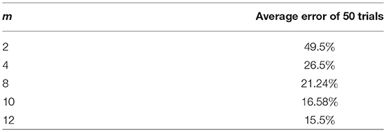
Table 3. Results of testing for “two intersecting circles” dataset.

4.3. Multiple Classification. Three Moons Dataset

Three moons dataset has been simulated from three half-circles by adding a gaussian noise with mean zero and deviation 0.14. Each half-circle contains 100 points so that n = 300. Figure 7 shows the classification results for m = 3 labeled points with other parameters M = 60; q = 0.9. The logarithmic plot of ε_k suggested by Algorithm 1 is shown at Figure 8. The big crosses correspond to the labeled data and other points are colored according to the constructed predictors. It can be seen that for m = 3 (just one labeled point per circle) the classification is performed correctly.

FIGURE 7

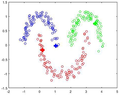
Figure 7. Classification of “three moons” dataset. The values of parameters are n = 300, m = 3, M = 60, p = 0.5, q=0.9.

FIGURE 8

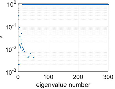
Figure 8. Logarithmic plot of adaptively chosen ε for three-moon dataset. The values of parameters are n = 300, m = 3, M = 60, p = 0.5, q=0.9.

4.4. Automatic Gender Identification

We also investigate the application of the proposed classification approach to the problem of automatic gender identification [22]. Having the audio recording of some speaker, the task is to determine the speaker's gender: male or female.

The gender classification task is usually performed on frame-by-frame basis as follows. The speech signal is divided onto the segments (frames) of 20 ms (160 samples for sampling frequency 8,000 Hz). For every such frame a set of voice parameters is calculated. It is necessary to use such parameters that provide distinct description of male and female voices. We used two-dimensional (d = 2) parameters vector consisting of pitch period T₀ [22] and difference of the first two line spectral frequencies (LSF) d = ω₂−ω₁ [for the definition, properties and computation of line spectral frequencies, see e.g., [23]].

For the training we used 240 audio recordings with total duration of 14 minutes. Male and female speakers of English and Russian languages were participating. The total number of the considered parameter vectors was 8,084 for male speakers and 8,436 for female speakers. To make the problem computationally tractable, we selected 128 “typical” parameter vectors both for male and female parts which were determined by k-means algorithm [24]. In the experiments l = 2 points both for “male” and “female” manifolds were labeled. Parameter ε was selected according to the proposed adaptive strategy. The value 1 of decision-making function was assigned to male speakers and the value −1 was assigned to female speakers.

The distribution of test parameters vectors and the results of their classification is shown in Figures 9, 10, respectively.

FIGURE 9

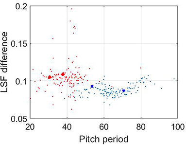
Figure 9. The distribution of 128 considered vectors for male (blue color) and female (red color) speakers. The four labeled points are marked.

FIGURE 10

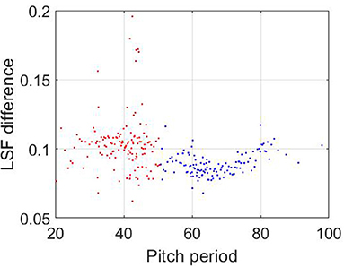
Figure 10. The results of the vectors' classification. Blue and red colors correspond to male and female speakers, respectively. The values of parameters are n = 128, m = 4, M = 30, p = 0.5, q=0.9.

Then the independent testing was performed on a set of 257 audio recordings including English, German, Hindi, Hungarian, Japanese, Russian, and Spanish speakers (all of these speakers did not take part in the training database). The decision male/female for an audio recording was made by majority of the decisions among all its frames. As the result of this independent testing, the classification errors for male and female speakers were 12.6 and 6.5%, respectively.

The examples of the decisions for frames of an audio recording are shown in Figures 11, 12 for male and female speakers, respectively. Each record was divided onto frames of 20 ms. On every frame the vector of features was calculated and then classified by the proposed approach. It can be seen that in the case of male speaker the most of the decision-making function values are grouped near value “1.” It provides correct classification of this record as “male.” Similarly, most of the decision-making function values for a female recording are grouped around are grouped around value “−1.”

FIGURE 11

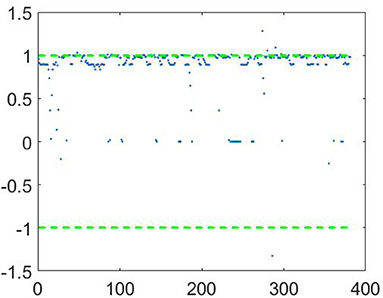
Figure 11. The example of decisions for frames of an audio recording of a male speaker.

FIGURE 12

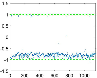
Figure 12. The example of decisions for frames of an audio recording of a female speaker.

The obtained results are promising and encourage to test the proposed approach on a larger variety of signals.

Data Availability

Publicly available datasets were analyzed in this study. This data can be found here: https://github.com/jaejun-yoo/shallow-DANN-two-moon-dataset.

Author Contributions

All authors listed have made a substantial, direct and intellectual contribution to the work, and approved it for publication .

Conflict of Interest Statement

The authors declare that the research was conducted in the absence of any commercial or financial relationships that could be construed as a potential conflict of interest.

Acknowledgments

SP and ES gratefully acknowledge the support of the consortium AMMODIT funded within EU H2020-MSCA-RICE via Grant H2020-MSCA-RISE-2014 project number 64567. The research of HM is supported in part by the Office of the Director of National Intelligence (ODNI), Intelligence Advanced Research Projects Activity (IARPA), via 2018-18032000002. This manuscript has been released as a Pre-Print at [25].

References

1. Micchelli CA, Pontil M. Learning the kernel function via regularization. JMachLearnRes. (2005) 6:10127–10134.

Google Scholar

2. Que Q, Belkin M, Wang Y. “Learning with Fredholm Kernels.” In: Ghahramani Z, Welling M, Cortes C, Lawrence ND, Weinberger KQ, editors. Advances in Neural Information Processing Systems 27, Montreal, QC: Curran Associates, Inc. (2014). p. 2951–2959. Available online at: http://papers.nips.cc/paper/5237-learning-with-fredholm-kernels.pdf

Google Scholar

3. Pereverzyev SV, Tkachenko P. Regularization by the Linear Functional Strategy with Multiple Kernels. Front. Appl. Math. Statist. (2017) 3:1. doi: 10.3389/fams.2017.00001

CrossRef Full Text | Google Scholar

4. Belkin M, Matveeva I, Niyogi P. “Regularization and semi-supervised learning on large graphs,” In: Shawe-Taylor J, Singer Y, editors. Learning Theory. Berlin; Heidelberg: Springer (2004). p. 624–638. doi: 10.1007/978-3-540-27819-1-43

CrossRef Full Text | Google Scholar

5. Belkin M, Niyogi P. Laplacian eigenmaps for dimensionality reduction and data representation. Neural Comput. (2003) 15:1373–1396. doi: 10.1162/089976603321780317

CrossRef Full Text | Google Scholar

6. Belkin M, Niyogi P. Semi-supervised learning on Riemannian manifolds. Mach Learn. (2004) 56:209–239. doi: 10.1023/B:MACH.0000033120.25363.1e

CrossRef Full Text | Google Scholar

7. Belkin M, Niyogi P, Sindhwani V. Manifold regularization: a geometric framework for learning from labeled and unlabeled examples. J Mach Learn Res. (2006) 7:2399–2434.

Google Scholar

8. Lafon SS. Diffusion Maps and Geometric Harmonics. Yale: Yale University (2004).

Google Scholar

9. Chui CK, Donoho DL. Special issue: diffusion maps and wavelets. Appl Comput Harmon Anal. (2006) 21:1–2. doi: 10.1016/j.acha.2006.05.005

CrossRef Full Text | Google Scholar

10. Bertozzi AL, Luo X, Stuart AM, Zygalakis KC. Uncertainty Quantification in the Classification of High Dimensional Data. SIAM/ASA J. Uncertainty Quantification (2017) 6:568–595. doi: 10.1137/17M1134214

CrossRef Full Text | Google Scholar

11. Jones PW, Maggioni M, Schul R. Universal local parametrizations via heat kernels and eigenfunctions of the Laplacian. Ann Acad Sci Fenn Math. (2010) 35:131–174. doi: 10.5186/aasfm.2010.3508

CrossRef Full Text | Google Scholar

12. von Luxburg U, Belkin M, Bousquet O. Consistency of spectral clustering. Ann Statist. (2008) 36:555–586. doi: 10.1214/009053607000000640

CrossRef Full Text | Google Scholar

13. Belkin M, Niyogi P. Convergence of Laplacian eigenmaps. Advances in Neural Information Processing Systems 19, Proceedings of the Twentieth Annual Conference on Neural Information Processing Systems, Vancouver (2007). p. 129.

Google Scholar

14. Maggioni M, Mhaskar HN. Diffusion polynomial frames on metric measure spaces. Appl Comput Harmon Anal. (2008) 24:329–353. doi: 10.1016/j.acha.2007.07.001

CrossRef Full Text | Google Scholar

15. Filbir F, Mhaskar HN. Marcinkiewicz–Zygmund measures on manifolds. J Complex. (2011) 27:568–596. doi: 10.1016/j.jco.2011.03.002

CrossRef Full Text | Google Scholar

16. Mhaskar HN. Eignets for function approximation on manifolds. Appl Comput Harm Anal. (2010) 29:63–87. doi: 10.1016/j.acha.2009.08.006

CrossRef Full Text | Google Scholar

17. Mhaskar HN. A generalized diffusion frame for parsimonious representation of functions on data defined manifolds. Neural Netw. (2011) 24:345–359. doi: 10.1016/j.neunet.2010.12.007

PubMed Abstract | CrossRef Full Text | Google Scholar

18. Ehler M, Filbir F, Mhaskar HN. Locally Learning Biomedical Data Using Diffusion Frames. J Comput Biol. (2012) 19:1251–1264. doi: 10.1089/cmb.2012.0187

PubMed Abstract | CrossRef Full Text | Google Scholar

19. Coifman RR, Hirn MJ. Diffusion maps for changing data. Appl Comput Harmon Anal. (2014) 36:79–107. doi: 10.1016/j.acha.2013.03.001

CrossRef Full Text | Google Scholar

20. Tikhonov AN, Glasko VB. Use of regularization method in non-linear problems. Zh Vychisl Mat Mat Fiz. (1965) 5:463–473.

Google Scholar

21. Lu S, Pereverzyev SV. Multi-parameter regularization and its numerical realization. Numer Math. (2011) 118:1–31. doi: 10.1007/s00211-010-0318-3

CrossRef Full Text | Google Scholar

22. Semenov V. Method for gender identification based on approximation of voice parameters by gaussian mixture models. Komp Mat. (2018) 2:109–118.

Google Scholar

23. Semenov V. A novel approach to calculation of line spectral frequencies based on inter-frame ordering property. In: 2006 IEEE International Conference on Acoustics Speech and Signal Processing Proceedings Toulouse (2006). p. 1072–1075. doi: 10.1109/ICASSP.2006.1660843

CrossRef Full Text | Google Scholar

24. Linde Y, Buzo A, Gray R. An algorithm for vector quantizer design. IEEE Trans Comm. (1980) 28:84–95.

Google Scholar

25. Mhaskar HN, Pereverzyev SV, Semenov VY, Semenova EV. Data based construction of kernels for semi-supervised learning with less labels. RICAM Preprint. (2018) 25:1–11.

Google Scholar