Simultaneous Structures in Convex Signal Recovery—Revisiting the Convex Combination of Norms

1. Introduction

The recovery of an unknown signal from a limited number of observations can be more efficient by exploiting compressibility and a priori known structure of the signal. This compressed sensing methodology has been applied to many fields in physics, applied math, and engineering. In the most common setting, the structure is given as sparsity in a known basis. To mention some more recent directions, block-, group-, and hierarchical sparsity, low-rankness in matrix or tensor recovery problems and also the generic concepts of atomic decomposition are important structures present in many estimation problems.

In most of these cases, convex relaxations render the inverse problems itself amenable to standard solvers at almost-optimal sampling rates and also show tractability from a theoretical perspective [1]. In one variant, one minimizes a regularizing function under the constraints given by the measurements. A good regularizing function, or just regularizer, gives a strong preference in the optimization toward the targeted structure. For instance, the ℓ₁-norm can be used to regularize for sparsity and the nuclear norm for low rankness of matrices.

1.1. Problem Statement

Let us describe the compressed sensing setting in more detail. We consider a linear measurement map ${A}:V\to {ℝ}^m$ on a d-dimensional vector space V ≅ ℝ^d define by its output components

$\begin{array}{ll}{A}{(x)}_i≔\langle a_i,x\rangle .& (1)\end{array}$

Throughout this work we assume the measurements to be Gaussian, i.e., $\langle a_i,e_j\rangle ~{N}(0,1)$ iid., where {e_j}_j∈[d] is an orthonormal basis of V. Moreover, we consider a given signal x₀ ∈ V, which yields the (noiseless) measurement vector

$\begin{array}{ll}y≔{A}(x_0).& (2)\end{array}$

We wish to reconstruct x₀ from ${A}$ and y in a way that is computationally tractable. Following a standard compressed sensing approach, we consider a norm $\parallel ·\parallel$_reg as regularizer. Specifically, we consider an outcome of the following convex optimization problem

$\begin{array}{ll}{x}_{\text{reg}}:=\text{arg min}\left\{{\Vert x\Vert }_{\text{reg}}: {A}(x)=y\right\}& (3)\end{array}$

as a candidate for a reconstruction of x₀, where we will choose $\parallel ·\parallel$_reg to be either the weighted sum or the weighted maximum of other norms (18). If computations related to $\parallel ·\parallel$_reg are also computationally tractable, Equation (3) can be solved efficiently. We wish that x_reg coincides with x₀. Indeed, when the number of measurements m is large enough (compared to the dimension d) then, with high probability over the realization of ${A}$, the signal is reconstructed, i.e., x₀ = x_reg. For instance, when m ≥ d then ${A}$ is invertible with probability 1 and, hence, the constraint ${A}(x)=y$ in (3) alone guarantees such a successful reconstruction.

However, when the signal is compressible, i.e., it can be described by fewer parameters than the dimension d, then one can hope for a reconstruction from fewer measurements by choosing a good regularizer $\parallel ·\parallel$_reg. For the case of Gaussian measurements, a quantity called the statistical dimension gives the number of measurements sufficient [2] and necessary [3] (see also [4, Corollary 4]) for a successful reconstruction. Therefore, much of this work is focused on such statistical dimensions.

Now we consider the case where the signal has several structures simultaneously. Two important examples are (i) simultaneously low rank and sparse matrices and (ii) tensors with several low rank matrizations. In such cases one often knows good regularizers for the individual structures. In this work, we address the question of how well one can use convex combinations of the individual regularizers to regularize for the combined structure.

1.2. Related Work

It is a standard practice to account for multiple simultaneous structures in convex optimization by combining different regularizers or constraints. The hope is to improve the sampling rate, i.e., to recover x₀ from fewer observations y. Unfortunately, when taking simple combinations of regularizers there are certain limitations on the improvement of sampling rate.

For the prominent example of entrywise sparse and low-rank matrices, Oymak et al. [5] showed that convex combinations of ℓ₁– and nuclear norm cannot improve the scaling of the sampling rate m in convex recovery. Mu et al. [4] considered linear combinations of arbitrary norms and derived more explicit and simpler lower bounds on the sampling rate using elegant geometric arguments.

In particular, this analysis also covers certain approaches to tensor recovery. It should be noted that low-rank tensor reconstruction using few measurements is notoriously difficult. Initially, it was suggested to use linear combinations of nuclear norms as a regularizer [6], a setting where the lower bounds [4] apply. Therefore, the best guarantee for tractable reconstructions is still a non-optimal reduction to the matrix case [4].

If one gives up on having a convex reconstruction algorithm, non-convex quasi-norms can be minimized that lead to an almost optimal sampling rate [7]. This reconstruction is for tensors of small canonical rank (a.k.a. CP rank). Also for this rank another natural regularizer might be the so-called tensor nuclear norm. This is another semi-norm for which one can find tractable semidefinite programming relaxations based on so-called θ-bodies [8]. These norms provide promising candidates for (complexity theoretically) efficient and guaranteed reconstructions.

Also following this idea of atomic norm decompositions [2], a single regularizer was found by Richard et al. [9] that yields again optimal sampling rates at the price that the reconstruction is not give by a tractable convex program.

1.3. Contributions and Outline

We discuss further the idea of taking convex combinations of regularizers from a convex analysis viewpoint. Moreover, we focus on the scenario where the weights in a maximum and also a sum of norms can depend on the unknown object x₀ itself, which reflects an optimal tuning of the convex program.

Based on tools established in Mu et al. [4], which may be not fully recognized in the community, we discuss simple convex combinations of regularizers. As already pointed out by Oymak et al. [5] an optimally weighted maximum of regularizers has the best sampling rate among such approaches. We follow this direction and discuss how sampling rates can be obtained in such setting. Specifically, we point out that the arguments leading to the lower bounds of Mu et al. [4] can also be used to obtain generic lower bounds for the maximum of norms, which implies similar bounds for the sum of norms (section 2). We also present an SDP characterization of dual norms for weighted sums and maxima and use them for numerically sampling the statistical dimension of descent cones, which correspond to the critical sampling rate [3].

In section 3 we discuss the prominent case of simultaneously sparse and low rank matrices. Here, our contributions are two-fold. We first show that the measurements satisfy a restricted isometry property (RIP) at a sampling rate that is essentially optimal for low rank matrices, which implies injectivity of the measurement map ${A}$. Then, second, we provide numerical results showing that maxima of regularizers lead to recovery results that show an improvement over those obtained by the optimally weighted sum of norms above an intermediate sparsity level.

Then, in section 4 we discuss the regularization for rank-1 tensors using combinations of matrix norms (extending the “square deal” [4] idea). In particular, we suggest to consider the maximum of several nuclear norms of “balanced” or “square deal” matrizations for the reconstruction of tensor products. We point out that the maximum of regularizers can lead to an improved recovery, often better than expected.

It is the hope that this work will contribute to more a comprehensive understanding of convex approaches to simultaneous structures in important recovery problems.

2. Lower Bounds for Convex Recovery With Combined Regularizers

In this section we review the convex arguments used by Mu et al. [4] to establish lower bounds for the required number of measurements when using a linear combination of regularizers.

2.1. Setting and Preliminaries

For a positive integer m we use the notation [m] ≔ {1, 2, …, m}. The ℓ_p-norm of a vector x is denoted by ∥x∥_ℓp and Schatten p-norm of a matrix X is denoted by ∥X∥_p. For p = 2 these two norms coincide and are also called Frobenius norm or Hilbert-Schmidt norm. With slight abuse of notation, we generally denote the inner product norm of a Hilbert space by $\parallel ·\parallel$_ℓ2. For a cone S and a vector g in a vector space with norm $\parallel ·\parallel$ we denote their induced distance by

$\begin{array}{ll}\parallel g-S\parallel ≔inf\left\{\parallel g-x\parallel :x\in S\right\}& (4)\end{array}$

The polar of a cone K is

$\begin{array}{ll}{K}^{\circ }≔\left\{y:\langle y,x\rangle \le 0\forall x\in K\right\}.& (5)\end{array}$

For a set S we denote its convex hull by conv(S) and the cone generated by S by cone(S) ≔ {τx : x ∈ S, τ > 0}. For convex sets C₁ and C₂ one has

$\begin{array}{ll}coneconv(C_1\cup C_2)=cone(C_1)+cone(C_2),& (6)\end{array}$

where “⊂” follows trivially from the definitions. In order to see “⊃” we write a conic combination z = ρx + σy ∈ cone(C₁) + cone(C₂) as $z=(\rho +\sigma )\left(\frac{\rho }{\rho +\sigma }x+\left(1-\frac{\rho }{\rho +\sigma }\right)y\right)$. The Minkowski sum of two sets C₁ and C₂ is denoted by C₁ + C₂ ≔ {x + y : x ∈ C₁, y ∈ C₂}. It holds that

$\begin{array}{ll}cone(C_1+C_2)\subseteq cone(C_1)+cone(C_2).& (7)\end{array}$

The subdifferential of a convex function f at base point x is denoted by ∂f(x). When f is a norm, f = $\parallel ·\parallel$, then the subdifferential is the set of vectors where Hölder's inequality is tight,

$\begin{array}{ll}\partial \parallel ·\parallel (x)=\left\{y:\langle y,x\rangle =\parallel x\parallel ,\Vert y{\Vert }^{\circ }\le 1\right\},& (8)\end{array}$

where ∥ y ∥° is the dual norm of $\parallel ·\parallel$ defined by $\parallel y{\parallel }^{\circ }≔{\sup }_{\parallel x\parallel =1}|\langle x,y\rangle |$. The descent cone of a convex function f at point x is [10, Definition 2.4]

$\begin{array}{ll}D(f,x)≔cone\left\{y:f(x+y)\le f(x)\right\}& (9)\end{array}$

and it holds that [10, Fact 3.3]

$\begin{array}{ll}D{(f,x)}^{\circ }=clcone\partial f(x),& (10)\end{array}$

where cl S denotes the closure of a set S. Let {f_i}_i∈[k] be proper convex functions such that the relative interiors of their domains have at least a point in common. Then

$\begin{array}{ll}\partial \left({\displaystyle \sum _{i\in \left[k\right]}}{\lambda }_i{f}_i\right)(x)={\displaystyle \sum _{i\in \left[k\right]}}{\lambda }_i\partial f_i(x).& (11)\end{array}$

A function $f≔{\max }_{i\in [k]}{f}_i$ that is the point-wise maximum of convex functions {f_i}_i∈[m] has the subdifferential [11, Corollary D.4.3.2]

$\begin{array}{ll}\partial f(x)=conv\left({\displaystyle \bigcup _{i:f_i(x)=f(x)}}\partial f_i(x)\right).& (12)\end{array}$

Hence, the generated cone is the Minkowski sum

$\begin{array}{ll}cone\partial f(x)={\displaystyle \sum _{i:f_i(x)=f(x)}}cone\partial f_i(x).& (13)\end{array}$

The Lipschitz constant of a function f w.r.t. to a norm $\parallel ·\parallel$ is the smallest constant L such that for all vectors x and x′

$\begin{array}{ll}|f(x)-f(x^{\prime })|\le L\parallel x-x^{\prime }\parallel .& (14)\end{array}$

Usually, $\parallel ·\parallel$ is an ℓ₂-norm, which also fits the Euclidean geometry of the circular cones defined below.

The statistical dimension of a convex cone K is given by (see e.g., [3, Proposition 3.1(4)])

$\begin{array}{ll}\delta (K)≔{\text{𝔼}}_g\left[{\parallel g-K^{\circ }\parallel }_{{\ell }_2}^2\right]& (15)\end{array}$

where g ~ N(0, 𝟙) is a Gaussian vector. The statistical dimension satisfies [3, Proposition 3.1(8)]

$\begin{array}{ll}\delta (K)+\delta (K^{\circ })=d& (16)\end{array}$

for any cone K ⊂ V in a vector space V ≅ ℝ^d. Now, let us consider a compressed sensing problem where we wish to recover a signal x₀ from m fully Gaussian measurements using a convex regularizer f. For small m, a successful recovery is unlikely and for large m the recovery works with overwhelming probability. Between these two regions of m one typically observes a phase transition. This transition is centered at a value given by the statistical dimension of the descent cone δ($D$(f, x₀)) of f at x₀ [3]. Thanks to Equation (10), this dimension can be calculated via the subdifferential of f,

$\begin{array}{ll}\delta (D(f,x_0))={\text{𝔼}}_g\left[{\parallel g-cone\partial f(x_0)\parallel }_{{\ell }_2}^2\right].& (17)\end{array}$

By ≳ and ≲ we denote the usual greater or equal and less or equal relations up to a positive constant prefactor and ∝ if both holds simultaneously. Then we can summarize that the convex reconstruction (3) requires exactly a number of measurements m ≳ δ($D$(f, x₀)), which can be calculated via the last equation.

2.2. Combined Regularizers

We consider the convex combination and weighted maxima of norms $\parallel ·\parallel$_(i), where i = 1, 2, …, k and set

$\begin{array}{ll}\begin{array}{c}{\parallel ·\parallel }_{\mu ,\text{max}}≔{\displaystyle \underset{i\in \left[k\right]}{max}}{\mu }_i\parallel ·{\parallel }_{(i)}\\ \parallel ·{\parallel }_{\lambda ,\text{sum}}≔{\displaystyle \sum _{i\in \left[k\right]}}{\lambda }_i\parallel ·{\parallel }_{(i)},\end{array}& (18)\end{array}$

where λ = (λ₁, …, λ_k) ≥ 0 and μ = (μ₁, …, μ_k) ≥ 0 are to be chosen later. Here, we assume that we have access to single norms of our original signal ∥x₀∥_(i) so that we can fine-tune the parameters λ and μ accordingly.

In Oymak et al. [5] lower bounds on the necessary number of measurements for the reconstruction (3) using general convex relaxations were derived. However, it has not been worked out explicitly what can be said in the case where one is allowed to choose the weights λ and μ dependending on the signal x₀. For the sum norm $\parallel ·\parallel$_λ,sum this case is covered by the lower bounds in Mu et al. [4]. Here, we will see that the arguments extend to optimally weighted max norms, i.e., $\parallel ·\parallel$_μ,max with μ being optimally chosen for a given signal.

A description of the norms dual to those given by (18) is provided in section 2.4.1.

2.3. Lower Bounds on the Statistical Dimension

The statistical dimension of the descent cone is obtained as Gaussian squared distance from the cone generated by the subdifferential (17). Hence, it can be lower bounded by showing (i) that the subdifferential is contained in a small cone and (ii) bounding that cone [4]. A suitable choice for this small cone is the so-called circular cone.

2.3.1. Subdifferentials and Circular Cones

We use the following statements from Amelunxen et al. [3] and Mu et al. [4, section 3] which show that subdifferentials are contained in circular cones. More precisely, we say that the angle between vectors x, z ∈ ℝ^d is θ if 〈z, x〉 = cos(θ) ∥z∥ _ℓ2∥x∥_ℓ2 and write in that case ∠(x, z) = θ. Then the circular cone with axis x and angle θ is defined as

$\begin{array}{ll}circ(x,\theta )≔\left\{z:\angle (x,z)\le \theta \right\}.& (19)\end{array}$

Its statistical dimension has a simple upper bound in terms of its dimension: For all x ∈ V ≅ ℝ^d and some θ ∈ [0, π/2] [4, Lemma 5]

$\begin{array}{ll}\delta (circ(x,\theta ))\le dsin{(\theta )}^2+2.& (20)\end{array}$

By the following argument this bound can be turned into a lower bound on the statistical dimension of descent cones and, hence, to the necessary number of measurements for signal reconstructions. The following two propositions summarize arguments made by Mu et al. [4].

Proposition 1 (Lower bound on descent cone statistical dimensions [4]). Let us consider a convex function f as a regularizer for the recovery of a signal $0\ne x_0\in V\cong {ℝ}^d$ in a d-dimensional space. If ∂f(x₀) ⊂ circ(x₀, θ) then

$\begin{array}{ll}\delta (D(f,x_0))\ge d{cos}^2\theta -2.& (21)\end{array}$

This statement is already implicitly contained in Mu et al. [4]. The arguments can be compactly summarized as follows.

Proof: With the polar of the descent cone (10), the assumption, and the statistical dimension of the polar cone (16) we obtain

$\begin{array}{ll}\delta (D(f,x_0))=d-\delta (cone\partial f(x_0))& (22)\end{array}$

$\begin{array}{ll}\ge d-\delta (circ(x_0,\theta ))& (23)\end{array}$

Hence, with the bound on the statistical dimension of the circular cone (20),

$\begin{array}{ll}\delta (D({\parallel ·\parallel }_{{\mu }^{*},\text{max}},x_0))\ge d(1-{sin}^2\theta )-2=d{cos}^2\theta -2.& (24)\end{array}$

□

Recall from (14) a norm f is L-Lipschitz with respect to the ℓ₂–norm on a (sub-)space V if

$\begin{array}{ll}f(x)\le L\Vert x\Vert {\ell }_2& (25)\end{array}$

for all x ∈ V. Note that this implies for the dual norm f° that

$\begin{array}{ll}\Vert x{\Vert }_{{\ell }_2}\le L{f}^{\circ }(x)& (26)\end{array}$

for all x ∈ V.

Proposition 2 ([4, section 3]). Let f be a norm on V ≅ ℝ^d that is L-Lipschitz with respect to the ℓ₂-norm on V. Then

$\begin{array}{ll}\partial f(x_0)\subseteq \left\{x:\frac{\langle x,x_0\rangle }{{\parallel x\parallel }_{{\ell }_2}{\parallel x_0\parallel }_{{\ell }_2}}\ge \frac{f(x_0)}{L{\parallel x_0\parallel }_{{\ell }_2}}\right\}=circ(x_0,\theta )& (27)\end{array}$

with $cos(\theta )=\frac{f(x_0)}{L{\parallel x_0\parallel }_{{\ell }_2}}$.

For sake of self-containedness we summarize the proof of Mu et al. [4, section 3].

Proof: The subdifferential of a norm f on V ≅ ℝ^d with dual norm f° is given by

$\begin{array}{ll}\partial f(x_0)=\left\{x:\langle x,x_0\rangle =f(x_0),f^{\circ }(x)\le 1\right\}.& (28)\end{array}$

Then, thanks to Hölder's inequality $\langle x,x_0\rangle \le f^{\circ }(x)f(x_0)$, we have for any subgradient x ∈ ∂f(x₀)

$\begin{array}{ll}\frac{\langle x,x_0\rangle }{{\parallel x\parallel }_{{\ell }_2}{\parallel x_0\parallel }_{{\ell }_2}}\stackrel{(28)}{=}\frac{f(x_0)}{{\parallel x_0\parallel }_{{\ell }_2}{\parallel x\parallel }_{{\ell }_2}}\stackrel{(26)}{\ge }\frac{f(x_0)}{L{\parallel x_0\parallel }_{{\ell }_2}{f}^{\circ }(x)}\stackrel{(28)}{\ge }\frac{f(x_0)}{L{\parallel x_0\parallel }_{{\ell }_2}}& (29)\end{array}$

This bound directly implies the claim. □

So together, Propositions 1 and 2 imply

$\begin{array}{ll}\delta (D(f,x_0))\ge \frac{d}{L^2}{\text{rank}}_f(x_0)-2,& (30)\end{array}$

where

$\begin{array}{ll}{\text{rank}}_f(x_0)≔\frac{f{(x_0)}^2}{{\parallel x_0\parallel }_{{\ell }_2}}& (31)\end{array}$

is the f-rank of x₀ (e.g., effective sparsity for f = $\parallel ·\parallel$_ℓ1 and effective matrix rank for f = $\parallel ·\parallel$₁).

2.3.2. Weighted Regularizers

A larger subdifferential leads to a smaller statistical dimension of the descent cone and, hence, to a reconstruction with a potentially smaller number of measurements in the optimization problems

$\begin{array}{ll}min{\parallel x\parallel }_{\mu ,\text{max}}\text{ subject to }{A}(x)=y& (32)\end{array}$

and

$\begin{array}{ll}\begin{array}{l}\min {\Vert x\Vert }_{\text{λ,sum}} \text{subject to }{A}(x)=y\hfill \end{array}& (33)\end{array}$

with the norms (18). Having the statistical dimension (17) in mind, we set

$\begin{array}{ll}{\delta }_{\text{sum}}(\lambda )≔{𝔼}_g\left[{\parallel g-cone\partial \parallel ·{\parallel }_{\lambda ,\text{sum}}(x_0)\parallel }_{{\ell }_2}^2\right]& (34)\end{array}$

$\begin{array}{ll}{\delta }_{max}(\mu )≔{𝔼}_g\left[{\parallel g-cone\partial {\parallel ·\parallel }_{\mu ,\text{max}}(x_0)\parallel }_{{\ell }_2}^2\right],& (35)\end{array}$

which give the optimal number of measurements in a precise sense [3, Theorem II]. Note that it is clear that δ_sum(λ) is continuous in λ.

Now we fix x₀ and consider adjusting the weights λ_i and μ_i depending on x₀. We will see the geometric arguments from Mu et al. [4] extend to that case. Oymak et al. [5, Lemma 1] show that the max-norm $\parallel ·\parallel$_μ,max with weights μ_i chosen as

$\begin{array}{ll}{\mu }_i^{*}≔\frac{1}{\parallel x_0{\parallel }_{(i)}}& (36)\end{array}$

has a better recovery performance than all other convex combinations of norms. With this choice the terms in the maximum (18) defining $\parallel ·\parallel$_μ,max are all equal. Hence, from the subdifferential of a maximum of functions (12) it follows that this choice of weights is indeed optimal. Moreover, the optimally weighted max-norm ${\parallel ·\parallel }_{{\mu }^{*},\text{max}}$ leads to a better (smaller) statistical dimension for x₀ than all sum-norms $\parallel ·\parallel$_λ,sum and, hence, indeed to a better reconstruction performance:

Proposition 3 (Optimally weighted max-norm is better than any sum-norm). Consider a signal x₀ and the corresponding optimal weights μ^* from (36). Then, for all possible weights λ ≽ 0 in the sum-norm, we have

$\begin{array}{ll}cone\partial \parallel ·{\parallel }_{\lambda ,sum}(x_0)\subset cone\partial {\parallel ·\parallel }_{{\mu }^{*},max}(x_0).& (37)\end{array}$

In particular, ${\delta }_{max}({\mu }^{*})\le {\delta }_{sum}(\lambda )$ for all λ ≽ 0.

Proof: Using (12) and (6) we obtain

$\begin{array}{lll}cone\partial {\parallel ·\parallel }_{\mu ,\text{max}}(x_0)& =coneconv\left({\displaystyle \bigcup _{i\in \left[k\right]}}\partial \parallel ·{\parallel }_{(i)}(x_0)\right)& (38)\end{array}$

$\begin{array}{ll}={\displaystyle \sum _{i\in \left[k\right]}}cone\partial \parallel ·{\parallel }_{(i)}(x_0)& (39)\end{array}$

with (11)

$\begin{array}{ll}\partial \parallel ·{\parallel }_{\lambda ,\text{sum}}(x_0)={\displaystyle \sum _{i\in \left[k\right]}}{\lambda }_i\partial \parallel ·{\parallel }_{(i)}(x_0).& (40)\end{array}$

Then (7) concludes the proof.□

Proposition 3 implies that if the max-norm minimization (32) with optimal weight (36) does not recover x₀, then the sum-norm minimization (33) can also not recover x₀ for any weight λ.

Now we will see that lower bounds on the number of measurements from Mu et al. [4, section 3] straightforwardly extend to the max-norm with optimal weights. These lower bound are obtained by deriving an inclusion into a circular cone. Combining Proposition 2 with (39) and noting that a Minkowski sum of circular cones (19) is just the largest circular cone yields the following:

Proposition 4 (Subdifferential contained in a circular cone). Let $0\ne x_0\in V\cong {ℝ}^d$ (signal) and $\parallel ·\parallel$_(i) be norms satisfying ∥x∥_(i) ≤ L_i∥x∥_ℓ2 for i ∈ [k] and for all x ∈ V. Then the subdifferential of

$\begin{array}{ll}{\parallel ·\parallel }_{{\mu }^{*},max}≔{\displaystyle \underset{i\in \left[k\right]}{max}}\frac{\parallel ·{\parallel }_{(i)}}{\parallel x_0{\parallel }_{(i)}}& (41)\end{array}$

satisfies

$\begin{array}{ll}\partial {\parallel ·\parallel }_{{\mu }^{*},max}(x_0)\subset circ(x_0,\theta )\text{ with }cos(\theta )={\displaystyle \underset{i\in \left[k\right]}{max}}\frac{\parallel x_0{\parallel }_{(i)}}{L_i{\parallel x_0\parallel }_{{\ell }_2}}.& (42)\end{array}$

In conjunction with Proposition 1 this yields the bound

$\begin{array}{ll}\delta (D({\parallel ·\parallel }_{{\mu }^{*},\text{max}},x_0))\ge \underset{i\in [k]}{\max }\frac{d{\Vert x_0\Vert }_{(i)}^2}{L_i^2{\Vert x_0\Vert }_{{\ell }_2}^2}-2.& (43)\end{array}$

Hence, upper bounds on the Lipschitz constants of the single norms yield a circular cone containing the subdifferential of the maximum, where the smaller the largest upper bound the smaller the circular cone. In terms of f-ranks it means that

$\begin{array}{ll}\delta (D({\parallel ·\parallel }_{{\mu }^{*},\text{max}},x_0))\ge {\displaystyle \underset{i\in \left[k\right]}{max}}\frac{d}{L_i^2}{\text{rank}}_{\parallel ·{\parallel }_{(i)}}(x_0)-2.& (44)\end{array}$

Now, Mu et al. [4, Lemma 4] can be replaced by this slightly more general proposition and the main lower bound [4, Theorem 5] on the number of measurements m still holds. The factor 16 in [4, Corollary 4] can be replaced by an 8 (see updated Arxiv version [12] of [3]). These arguments [specifically, [12, (7.1) and (6.1)] with λ ≔ δ(C) − m] show the following for the statistical dimension δ of the descent cone. The probability of successful recovery for m ≤ δ is upper bounded by p for all $m\le \delta -\sqrt{8\delta ln(4/p)}$. Conversely, the probability of unsuccessful recovery for m ≥ δ is upper bounded by q for any $m\ge \delta +\sqrt{8mln(4/q)}$, so in particular, for any $m\ge \delta +\sqrt{8dln(4/q)}$. Moreover, this yields the following implication of Amelunxen et al. [3]:

Theorem 5 (Lower bound). Let $\parallel ·\parallel$_(i) be norms satisfying ∥x∥_(i) ≤ L_i ∥x∥_ℓ2 for i ∈ [k] and for all x ∈ V. Fix $0\ne x_0\in V\cong {ℝ}^d$ (signal) and set

$\begin{array}{ll}\kappa ≔{\displaystyle \underset{i\in \left[K\right]}{min}}\frac{d{\Vert x_0\Vert }_{(i)}^2}{L_i^2{\Vert x_0\Vert }_{{\ell }_2}^2}-2\text{ (min. number of measurements)}.& (45)\end{array}$

Consider the optimally weighted max-norm (41). Then, for all m ≤ κ, the probability $p_{\mathit{\text{success}}}^{\mathit{\text{max}}}$ that x₀ is the unique minimizer of the reconstruction program (32) is bounded by

$\begin{array}{ll}{p}_{\text{success}}^{\text{max}}\le 4exp\left(-\frac{{(\kappa -m)}^2}{8\kappa }\right).& (46)\end{array}$

We will specify the results in more detail for the sparse and low-rank case in Corollary 8 and an example for the tensor case in Equation (100).

2.4. Estimating the Statistical Dimension Via Sampling and Semidefinite Programming

Often one can characterize the subdifferential of the regularizer by a semidefinite program (SDP). In this case, one can estimate the statistical dimension via sampling and solving such SDPs.

In more detail, in order to estimate the statistical dimension (17) for a norm f, we sample the Gaussian vector $g~{N}(0,\mathrm{𝟙})$, calculate the distance ${\parallel g-cone\partial f(x_0)\parallel }_{{\ell }_2}^2$ using the SDP-formulation of ∂f(x₀) and take the sample average in the end. In order to do so, we wish to also have an SDP characterization of the dual norm ∂f° of f, which provides a characterization of the subdifferential (8) of f.

In the case when the regularizer function f is either $\parallel ·\parallel$_μ,max or $\parallel ·\parallel$_λ,sum, where the single norms $\parallel ·\parallel$_(i) have simple dual norms, we can indeed obtain such an SDP characterization of the dual norm f°.

2.4.1. Dual Norms

It will be convenient to have explicit formulae for the dual norms to the combined regularizers defined in section 2.2 [13].

Lemma 6 (Dual of the maximum/sum of norms). Let $\parallel ·\parallel$_(i) be norms (i ∈ [k]) and denote by $\parallel ·\parallel$_μ,max and $\parallel ·\parallel$_λ,sum their weighted maximum and weighted sum as defined in (18). Then their dual norms are given by

$\begin{array}{ll}{\Vert y\Vert }_{\mu ,\text{max}}^{\circ }=\text{inf}\left\{{\displaystyle \sum _{i=1}^k\frac{1}{{\mu }_i}}{\Vert x_i\Vert }_{(i)}^{°}:y={\displaystyle \sum _{i=1}^k{x}_i}\right\}& (47)\end{array}$

$\begin{array}{ll}{\Vert y\Vert }_{\text{λ},sum}^{\circ }=\text{inf}\left\{\underset{i\in [k]}{\text{max}}\frac{1}{{\lambda }_i}{\Vert x_i\Vert }_{(i)}^{°}:y={\displaystyle \sum _{i=1}^k{x}_i}\right\}.& (48)\end{array}$

For the proof of the lemma we use the notation from the convex analysis book by Rockafellar [14]. For an alternative more elementary proof see [15].

Let C ⊂ ℝ^d be a convex set. Then its support function is defined by

$\begin{array}{ll}{\delta }_C^{*}(x)≔{\displaystyle \underset{y\in C}{sup}}\langle x,y\rangle & (49)\end{array}$

and its indicator function by

$\begin{array}{ll}{\delta }_C(x)≔\{\begin{array}{cc}0\hfill & \text{if }x\in C\hfill \\ \infty & \text{otherwise.}\end{array}& (50)\end{array}$

If C contains the origin, then we define its gauge function by

$\begin{array}{ll}{\gamma }_C(x)≔min\left\{\lambda \in ℝ:x\in \lambda C\right\}& (51)\end{array}$

and the polar of C to be

$\begin{array}{ll}{C}^{\circ }≔\left\{y:\langle y,x\rangle \le 1\forall x\in C\right\}.& (52)\end{array}$

[Note that while formally different, this definition is consistent with the polar of a cone introduced in (5).] The polar of a gauge function γ is denoted by γ°(y) := inf {λ ≥ 0 : 〈y, x〉 ≤ λγ(x)} and the convex conjugate of a function (Fenchel-Legendre dual) f by f^*. The infimal convolution of convex functions f and g is defined by $f\square g(x)≔{inf}_y\left\{f(x-y)+g(y)\right\}$.

There are all sorts of rules [14] that we will use. Let f and g be lower semi-continuous convex functions and C₁, C₂ and B be convex sets where B contains the origin. Then f^** = f, ${\gamma }_B^{\circ \circ }={\gamma }_B$, B^°° = c1 B, ${\delta }_{C_1}^{*}+{\delta }_{C_2}^{*}={\delta }_{C_1+C_2}^{*}$, (f□g)^* = f^*+g^*, ${\delta }_B^{*}={\gamma }_{B^{\circ }}$, and ${({\delta }_C)}^{*}={\delta }_C^{*}$.

Proof of Lemma 6: For the sake of better readability we focus on the case k = 2. The general case follows analogously.

In order to establish the statement of the lemma we will use the fact that the norms are the gauge functions of their unit balls, i.e., $\parallel ·\parallel$_(i) = γ_Bi with B_i := {x: ∥x∥_(i) ≤ 1}. For the proofs, however, let B_i be closed convex sets containing the origin (they do not need to satisfy B_i = −B_i, as is the case for norms).

We begin with the polar of the sum (48). Note that, in general, the “polar body (K + L)° of a [Minkowski] sum of convex bodies has no plausible interpretation in terms of K°, L°” [16]. However, we can still find a useful expression for the dual norm:

$\begin{array}{lll}\hfill {({\gamma }_{B_1}+{\gamma }_{B_2})}^{°}& ={({\delta }_{B_1^{°}}^{\ast }+{\delta }_{B_2^{°}}^{\ast })}^{°}\hfill & ={({\delta }_{B_1^{°}+B_2^{°}}^{\ast })}^{°}\hfill \\ \hfill & ={\left({\gamma }_{(B_1^{°}+B_2^{°})°}\right)}^{°}\hfill & ={\gamma }_{B_1^{°}+B_2^{°}},\hfill & (53)\end{array}$

so that

$\begin{array}{ll}{({\gamma }_{B_1}+{\gamma }_{B_2})}^{\circ }(a)={\displaystyle \underset{a=x+y}{min}}max\left\{{\gamma }_{B_1^{\circ }}(x),{\gamma }_{B_2^{\circ }}(y)\right\},& (54)\end{array}$

which implies the statement (48).

In order to establish the polar of the maximum (47) we start with the identity

$\begin{array}{ll}{\gamma }_{B_1\cap B_2}=max\left\{{\gamma }_{B_1},{\gamma }_{B_2}\right\}& (55)\end{array}$

to obtain

$\begin{array}{lll}\hfill \max {\{{\gamma }_{B_1},{\gamma }_{B_2}\}}^{°}& =\hfill & {\delta }_{B_1\cap B_2}^{\ast }={({\delta }_{B_1\cap B_2})}^{\ast }\hfill \\ \hfill & =\hfill & {({\delta }_{B_1}+{\delta }_{B_2})}^{\ast }={\left({\gamma }_{B_1^{°}}^{\ast }+{\gamma }_{B_2^{°}}^{\ast }\right)}^{\ast }\hfill \\ \hfill & =\hfill & {\gamma }_{B_1^{°}}\square {\gamma }_{B_2^{°}},\hfill & (56)\end{array}$

so that

$\begin{array}{ll}max{\left\{{\gamma }_{B_1},{\gamma }_{B_2}\right\}}^{\circ }(a)={\displaystyle \underset{a=y+z}{min}}\left\{{\gamma }_{B_1}^{\circ }(y)+{\gamma }_{B_2}^{\circ }(z)\right\},& (57)\end{array}$

which proves the identity (47).□

2.4.2. Gaussian Distance as SDP

We were aiming to estimate the statistical dimension (17) by sampling over Gaussian vectors g and the corresponding SDP outcomes. For any vector g the distance to the cone generated by the subdifferential of a norm f is

$\begin{array}{l}{\parallel g-cone\partial f(x_0)\parallel }_{{\ell }_2}\\ =min\left\{{\parallel g-\tau x\parallel }_{{\ell }_2}:\tau \ge 0,\langle x,x_0\rangle =f(x_0),f^{\circ }(x)\le 1\right\}& (58)\end{array}$

$\begin{array}{ll}=min\left\{{\parallel g-x\parallel }_{{\ell }_2}:\tau \ge 0,\langle x,x_0\rangle =\tau f(x_0),f^{\circ }(x)\le \tau \right\}& (59)\end{array}$

For f = $\parallel ·\parallel$_λ,sum we use its polar (48) to obtain

$\begin{array}{ll}\hfill & \Vert g-\text{cone }\partial {\Vert \cdot \Vert }_{\text{λ,sum}}(x_0){\Vert }_{{\ell }_2}\hfill \\ \hfill =& \underset{\tau ,x}{\min }\{{\Vert g-\tau x\Vert }_{{\ell }_2}:\tau \ge 0,\langle x,x_0\rangle ={\Vert x_0\Vert }_{\text{λ,sum}},\hfill \\ \hfill & \underset{{\left\{x_i\right\}}_{i=1}^{[k]}}{\inf }\left\{\underset{{ }_{i\in [k]}}{\max }\frac{{\Vert x_i\Vert }_{(i)}^{°}}{{\text{λ}}_i}:x={\displaystyle \sum _{i=1}^k{x}_i}\right\}\le 1\}\hfill & (60)\end{array}$

$\begin{array}{ll}\hfill =& \underset{{ }_{\tau ,x,{\left\{x_i\right\}}_{i=1}^{[k]}}}{\text{min}}\{{\Vert g-\tau x\Vert }_{{\ell }_2}:\tau \ge 0,\langle x,x_0\rangle ={\Vert x_0\Vert }_{\text{λ},\text{sum}},\hfill \\ \hfill & \frac{{\Vert x_i\Vert }_{(i)}^{°}}{{\text{λ}}_i}\le 1,x={\displaystyle \sum _{i=1}^k{x}_i}\},\hfill & (61)\end{array}$

where one needs to note that an optimal feasible point of (60) also yields an optimal feasible point of (61) and vice versa. But this implies that

$\begin{array}{ll} \hfill & {\Vert g-\text{ cone }\partial {\Vert \cdot \Vert }_{\text{λ,sum}}(x_0)\Vert }_{{\ell }_2}\hfill \\ =\hfill & \underset{\tau ,{\left\{x_i\right\}}_{i=1}^{[k]}}{\min }\{{\Vert g-{\displaystyle \sum _i{x}_i}\Vert }_{{\ell }_2}:{\displaystyle \sum _i\langle x_i,x_0\rangle }=\tau {\Vert x_0\Vert }_{\text{λ,sum}},\hfill \\ \hfill & {\Vert x_i\Vert }_{(i)}^{°}\le \tau {\text{λ}}_i,\tau \ge 0\}.\hfill & (62)\end{array}$

For the maximum of norms regularizer we again choose the optimal weights (36) to ensure that all norms are active, i.e.,

$\begin{array}{ll}{\mu }_i^{*}\parallel x_0{\parallel }_{(i)}={\parallel x_0\parallel }_{{\mu }^{*},\text{max}}.& (63)\end{array}$

Then we use the subdifferential expression (13) for a point-wise maximum of functions to obtain

$\begin{array}{l}{\Vert g-\text{ cone }\partial {\Vert \cdot \Vert }_{{\mu }^{\ast },\max }(x_0)\Vert }_{{\ell }_2}={\Vert g-{\displaystyle \sum _{i=1}^k\text{cone }}\partial {\Vert \cdot \Vert }_{(i)}(x_0)\Vert }_{{\ell }_2}\\ =\underset{{ }_{{\left\{\tau \right\}}_{i=1}^{[k]},{\left\{x_i\right\}}_{i=1}^{[k]}}}{\min }\{{\Vert g-{\displaystyle \sum _i{x}_i}\Vert }_{{\ell }_2}:\langle x_i,x_0\rangle ={\tau }_i{\Vert x_0\Vert }_{{\mu }^{\ast },\max },\\ {\Vert x_i\Vert }_{(i)}^{°}\le {\tau }_i{\mu }_i^{\ast },{\tau }_i\ge 0\}.& (64)\end{array}$

In the case that $\parallel x_i{\parallel }_{(i)}^{\circ }$ are ℓ_∞-norms or spectral norms these programs can be written as SDPs and be solved by standard SDP solvers.

3. Simultaneously Sparse and Low-Rank Matrices

A class of structured signals that is important in many applications are matrices which are simultaneously sparse and of low rank. Such matrices occur in sparse phase retrieval¹ [5, 17, 18], dictionary learning and sparse encoding [19], sparse matrix approximation [20], sparse PCA [21], bilinear compressed sensing problems like sparse blind deconvolution [22–27] or, more general, sparse self-calibration [28]. For example, upcoming challenges in communication engineering and signal processing require efficient algorithms for such problems with theoretical guarantees [29–31]. It is also well-known that recovery problems related to simultaneous structures like sparsity and low-rankness are at optimal rate often as hard as the classical planted/hidden clique problems, see for example [32] for further details and references.

3.1. Setting

We consider the d = n₁ · n₂–dimensional vector space $V={𝕂}^{n_1\times n_2}$ of n₁ × n₂-matrices with components in the field 𝕂 being either ℝ or ℂ. The space V is equipped with the Hilbert-Schmidt inner product defined by

$\begin{array}{ll}\langle X,Y\rangle ≔\text{Tr}(X^{†}Y).& (65)\end{array}$

Our core problem is to recover structured matrices from m linear measurements of the form $y={A}(X)$ with a linear map ${A}:{𝕂}^{n_1\times n_2}\to {𝕂}^m$. Hence, a single measurement is

$\begin{array}{ll}{y}_i={A}{(X)}_i=\langle A_i,X\rangle .& (66)\end{array}$

It is clear that without further a-priori assumptions on the unknown matrix X we need m ≥ d = n₁ · n₂ measurements to be able to successfully reconstruct X.

As additional structure, we consider subsets of V containing simultaneously low-rank and sparse matrices. However, there are different ways of combining low-rankness and sparsity. For example one could take matrices of rank r with different column and row sparsity, i.e., meaning that there are only a small number of non-zero rows and columns. Here, we consider a set having even more structure which is motivated by atomic decomposition [2]. Recall, that the rank of a matrix X can be defined as its “shortest description” as

$\begin{array}{ll}\text{rank}(X)≔\text{min}\left\{r:X={\displaystyle \sum _{i=1}^r{x}_i{y}_i^{†}},x_i\in {ℝ}^{n_1},y_i\in {ℝ}^{n_2}\right\}& (67)\end{array}$

and the vectors {x_i} and {y_i} can be required to be orthogonal, respectively. This characterization giving rise to the nuclear norm $\parallel ·\parallel$₁ as the corresponding atomic norm, see Chandrasekaran et al. [2] for a nice introduction to inverse problems from this viewpoint. Restricting the sets of feasible vectors {x_i} and {y_i} yields alternative formulations of rank. In the case of sparsity, one can formally ask for a description in terms of (s₁, s₂)-sparse atoms:

$\begin{array}{ll}{\text{rank}}_{s_1,s_2}(X)≔\text{min}\left\{r:X={\displaystyle \sum _{i=1}^r{x}_i{y}_i^{†}},{\Vert x_i\Vert }_{{\ell }_0}\le s_1,{\Vert y_i\Vert }_{{\ell }_0}\le s_2\right\},& (68)\end{array}$

where ∥x∥_ℓ0 denotes the number of non-zero elements of a vector x. The idea of the corresponding atomic norm [2] has been worked for the sparse setting by Richard et al. [9]. Note that, compared to (67), we do not require that ${\left\{x_i\right\}}_{i=1}^r$ and ${\left\{y_i\right\}}_{i=1}^r$ are orthogonal.

We say that a matrix $X\in {𝕂}^{n_1\times n_2}$ is simultaneously (s₁, s₂)-sparse and of rank r if it is in the set

$\begin{array}{ll}{𝕄}_{r,s_1,s_2}^{n_1\times n_2}≔\left\{{\displaystyle \sum _{i=1}^r}{x}_i{y}_i^{†}:\parallel x_i{\parallel }_0\le s_1,\parallel y_i{\parallel }_0\le s_2\right\}.& (69)\end{array}$

Our model differs to the joint-sparse setting as used in Lee et al. [22], since the vectors ${\left\{x_i\right\}}_{i=1}^r$ and ${\left\{y_i\right\}}_{i=1}^r$ may have individual sparse supports and need not to be orthogonal. Definition (69) fits more into the sparse model considered also in Fornasier et al. [33].

By e_i we denote i-th canonical basis vector and define row-support supp₁(X) and column-support supp₂(X) of a matrix X as

$\begin{array}{ll}{\text{supp}}_1(X)≔\left\{i:\Vert X^{†}{e}_i\Vert >0\right\},{\text{supp}}_2(X)={\text{supp}}_1(X^{†}).& (70)\end{array}$

Obviously, the matrices ${𝕄}_{r,s_1,s_2}^{n_1\times n_2}$ are then at most k₁-column-sparse and k₂-row-sparse (sometimes also called as joint-sparse), i.e.,

$\begin{array}{ll}\left|{\text{supp}}_1(X)\right|\le r{s}_1=:k_1\text{ and }\left|{\text{supp}}_2(X)\right|\le r{s}_2=:k_2& (71)\end{array}$

but not strictly $k_1{k}_2=r^2{s}_1{s}_2$–sparse². Since we have sums of r different (s₁, s₂)-sparse matrices and there are at most r(s₁ · s₂) non-zero components. Note that a joint (s₁, s₂)-row and column sparse matrix has only s₁ · s₂ non-zero entries. Hence, considering this only from the perspective of sparse vectors, we expect that up to logarithmic terms recovery can be achieved from m ∝ r(s₁ · s₂) measurements. On the other hand, solely from a viewpoint of low-rankness, m ∝ r (n₁ + n₂) measurements also determine an n₁ × n₂-matrix of rank r. Combining both gives therefore m ∝ r min(s₁s₂, n₁ + n₂).

On the other hand, these matrices are determined by at most r(s₁ + s₂) non-zero numbers. Optimistically, we therefore hope that already m ≲ r(s₁ + s₂) sufficiently diverse observations are enough to infer on X which is substantially smaller and scales additive in s₁ and s₂. In the next part we will discuss that this intuitive parameter counting argument is indeed true in the low-rank regime $r\lesssim logmax(\frac{n_1}{r{s}_1},\frac{n_2}{r{s}_2})$. A generic low-dimensional embedding of this simultaneously sparse and low-rank structure into 𝕂^m for m ∝ r(s₁ + s₂) via a Gaussian map ${A}$ is stably injective.

3.2. About RIP for Sparse and Low-Rank Matrices

Intuitively, (s₁, s₂)–sparse rank-r matrices can be stably identified from y if ${𝕄}_{r,s_1,s_2}^{n_1\times n_2}$ is almost-isometrically mapped into 𝕂^m, i.e., distances between different matrices are preserved up to small error during the measurements process. Note that we have the inclusion

$\begin{array}{ll}{𝕄}_{r,s_1,s_2}^{n_1\times n_2}-{𝕄}_{r,s_1,s_2}^{n_1\times n_2}\subset {𝕄}_{2r,s_1,s_2}^{n_1\times n_2}.& (72)\end{array}$

Since ${A}$ is linear it is therefore sufficient to ensure that norms $\Vert {A}(X)\Vert ~\Vert X\Vert$ are preserved for $X\in {𝕄}_{2r,s_1,s_2}^{n_1\times n_2}$. We say that a map ${A}:{𝕂}^{n_1\times n_2}\to {𝕂}^m$ satisfies (r, s₁, s₂)-RIP with constant δ if

$\begin{array}{ll}{\displaystyle \underset{\begin{array}{c}X\in {S}\end{array}}{sup}}{\displaystyle \parallel {{A}}^{†}{A}(X)-X{\parallel }_2}\le \delta & (73)\end{array}$

holds, where the supremum is taken over all ${S}=\left\{X\in {𝕄}_{r,s_1,s_2}^{n_1\times n_2}:\Vert X{\Vert }_2=1\right\}$ and ${{A}}^{†}$ denotes the adjoint of ${A}$ (defined in the canonical way with respect to the Hilbert-Schmidt inner product). By $\delta ({A})$ we always denote the smallest value δ such that above condition holds. Equivalently, we have

$\begin{array}{ll}(1-\delta ({A}))\parallel X{\parallel }_2^2\le {\displaystyle \parallel {A}(X){\parallel }_{{\ell }_2}^2}\le (1+\delta ({A}))\parallel X{\parallel }_2^2\forall X\in {𝕄}_{r,s_1,s_2}^{n_1\times n_2}.& (74)\end{array}$

A generic result, based on the ideas of Baraniuk et al. [34], Candes and Plan [35], and Recht et al. [36], has been presented already in Jung and Walk [29]. It shows that a random linear map ${A}$ which concentrates uniformly yields the RIP property (74) with overwhelming probability (exponential small outage) once the number of measurements are in the order of the metric entropy measuring the complexity of the structured set ${S}$. In the case of simultaneous low rank and sparse matrices this quantity scales (up to logarithmic terms) additively in the sparsity, as desired. A version for rank-r matrices where ${\left\{x_i\right\}}_{i=1}^r$ and ${\left\{y_i\right\}}_{i=1}^r$ in (69) are orthonormal sets having joint-sparse supports has been sketched already in Lee et al. [22, Theorem III.7], i.e., ${A}$ with iid Gaussian entries acts almost isometrically in this case for $m\gtrsim {\delta }^{-2}r(s_1+s_2)$ with probability at least $1-exp(-c_2{\delta }^{2}m)$, c₂ being an absolute constant. Another RIP perspective has been considered in Fornasier et al. [33] where the supremum in (73) is taken over effectively sparse (${\left\{x_i\right\}}_{i=1}^r$ and ${\left\{y_i\right\}}_{i=1}^r$ in (69) are now only well–approximated by sparse vectors) rank-r matrices X with ${\left({\sum }_{i=1}^r{\Vert x_i\Vert }_{l_2}^2{\Vert y_i\Vert }_{l_2}^2\right)}^{1/2}$ (implying ${\Vert X\Vert }_2\le \sqrt{r}\cdot \Gamma$). More precisely, for $m\gtrsim {\Delta }^{-2}r(s_1+s_2)$ with Δ ∈ (0, 1) an operator ${A}$ with iid. centered sub-Gaussian entries acts almost-isometrically with probability at least 1 − 2 exp(−C′ Δm) at δ = ΔΓ²r and C′ is an absolute constant. Note that this probability is slightly weaker.

We provide now a condensed version of the generic statement in Jung and Walk [29]. More precisely, RIP (74) is satisfied with high probability for a random linear map ${A}$ that has uniformly sub-Gaussian marginals:

Theorem 7 (RIP for sub-Gaussian measurements). Let ${A}:{ℝ}^{n_1\times n_2}\to {ℝ}^m$ be a random linear map which for given c > 0 and 0 < δ < 1 fulfills $\mathbb{P}[|{\parallel {A}(X)\parallel }_{{\ell }_2}-{\Vert X\Vert }_2|\le \frac{\delta }{2}{\Vert X\Vert }_2]\ge 1-{\text{e}}^{-c{\delta }^{2}m}$ uniformly for all $X\in {ℝ}^{n_1\times n_2}$. If

$\begin{array}{ll}m\ge c^{″}{\delta }^{-2}r(s_1+s_2)\left(1+logmax\left\{\frac{n_1}{r{s}_1},\frac{n_2}{r{s}_2}\right\}+rlog(9·4/\delta )\right)& (75)\end{array}$

then ${A}$ satisfies (r, s₁, s₂)-RIP with constant $\delta ({A})\le \delta$ with probability $\ge 1-{\text{e}}^{-\tilde{c}{\delta }^{2}m}$. Here, $\tilde{c}>0$ is an absolute constant and c″ is a constant depending only on δ and $\tilde{c}$.

Clearly, standard Gaussian measurement maps ${A}$ fulfill the concentration assumption in the theorem. More general sub-Gaussian maps are included as well, see here also the discussion in Jung and Walk [29]. The proof steps are essentially well-known. For the sake of self-containedness we review the steps having our application in mind.

Proof: First, we construct a special ϵ-net ${R}\subset {S}$ for ${S}=\{X\in {𝕄}_{r,s_1,s_2}^{n_1\times n_2}:{\Vert X\Vert }_2=1\}$. By this we mean a set such that for each $X\in {S}$ we have some $R=R(X)\in {R}$ such that ‖X − R‖₂ ≤ ϵ. Since the matrices $X\in {𝕄}_{r,s_1,s_2}^{n_1\times n_2}$ are k₁ := rs₁ row-sparse and k₂ ≔ rs₂ column-sparse there are

$\begin{array}{ll}L=\left(\begin{array}{c}{n}_1\\ k_1\end{array}\right)\left(\begin{array}{c}{n}_2\\ k_2\end{array}\right)\le {\left(\frac{\text{e}{n}_1}{k_1}\right)}^{k_1}{\left(\frac{\text{e}{n}_2}{k_2}\right)}^{k_2}\le {\left(\text{e }\max \left\{\frac{n_1}{k_1},\frac{n_2}{k_2}\right\}\right)}^{k_1+k_2}& (76)\end{array}$

different combinations for the row support T₁ ⊂ [n₁] and column support T₂ ⊂ [n₂] with |T₁| = k₁ and |T₂| = k₂. For each of these canonical matrix subspaces supported on T₁ × T₂, we consider matrices of rank at most r. From Candes and Plan [35, Lemma 3] it is known that there exists an ϵ-net for k₁ × k₂ matrices of rank r of cardinality ${(9/ϵ)}^{(k_1+k_2)r}$ giving therefore

$\begin{array}{ll}log|{R}|\le \left(k_1+k_2\right)\left(1+logmax\left\{\frac{n_1}{k_1},\frac{n_2}{k_2}\right\}+rlog(9/ϵ)\right).& (77)\end{array}$

In other words, up to logarithmic factors, this quantity also reflects the intuitive parameter counting. The net construction also ensures that for each $X\in {S}$ and close by net point R = R(X) we have | supp₁(X − R)| ≤ k₁ and | supp₂(X − R)| ≤ k₂. However, note that in non-trivial cases rank(R − X) = 2r meaning that $(R-X)/\Vert R-X{\Vert }_2\notin {S}$. Still, using a singular value decomposition one can find R − X = X₁ + X₂ with 〈X₁, X₂〉 = 0 for some $X_1/{\Vert X_1\Vert }_2\in {S}$ and $X_2/{\Vert X_2\Vert }_2\in {S}$. To show RIP, we define the constant

$\begin{array}{ll}A\text{:}={\displaystyle \underset{X\in {S}}{max}}|{\parallel {A}(X)\parallel }_{{\ell }_2}-1|.& (78)\end{array}$

For some $X\in {S}$ and close by net point $R=R(X)\in {R}$ and let us consider δ such that ${\parallel {A}(R)\parallel }_{{\ell }_2}-1|\le \delta /2$. Then,

$\begin{array}{ll}\begin{array}{l}|\Vert {A}(X){\Vert }_{{\ell }_2}-1|\le |{\parallel {A}(X)\parallel }_{{\ell }_2}-{\parallel {A}(R)\parallel }_{{\ell }_2}|+|{\parallel {A}(R)\parallel }_{{\ell }_2}-1|\\ \le \Vert {A}(X-R){\Vert }_{{\ell }_2}+\frac{\delta }{2}\le \Vert {A}(X_1){\Vert }_{{\ell }_2}+\Vert {A}(X_2){\Vert }_{{\ell }_2}+\frac{\delta }{2}\\ \le (1+A)(\Vert X_1{\Vert }_2+\Vert X_2{\Vert }_2)+\frac{\delta }{2}=(1+A)\Vert X_1+X_2{\Vert }_2+\frac{\delta }{2}\\ =(1+A)\Vert X-R{\Vert }_2+\frac{\delta }{2}\le (1+A)ϵ+\frac{\delta }{2}.\end{array}& (79)\end{array}$

Now we choose $\tilde{X}\in {S}$ satisfying $A=|{\Vert {A}\left(\tilde{X}\right)\Vert }_{l_2}-1|$ [${S}$ in (78) is compact]. For such an $\tilde{X}$ we also have

$\begin{array}{ll}\begin{array}{c}A=|\Vert {A}(\tilde{X}){\Vert }_{{\ell }_2}-1|\le (1+A)ϵ+\frac{\delta }{2}.\end{array}& (80)\end{array}$

Requiring that the right hand side is bounded by δ and solving this inequality for A (assuming ϵ < 1) we find that indeed $A\le \frac{ϵ+\delta /2}{1-ϵ}\le \delta$ whenever ϵ ≤ δ/(2 + 2δ). In particular we can choose δ < 1 and we set ϵ = δ/4. Therefore, Equation (77) yields

$\begin{array}{ll}\begin{array}{c}log|{R}|\le (k_1+k_2)\left(1+logmax\left\{\frac{n_1}{k_1},\frac{n_2}{k_2}\right\}+rlog(9·4/\delta )\right).\end{array}& (81)\end{array}$

Using the assumption $\mathbb{P}\left[|{\Vert {A}(X)\Vert }_{{\ell }_2}-{\Vert X\Vert }_2|\le \delta /2{\Vert X\Vert }_2\right]\ge 1$ −e^−cδ2m and the union bound $\mathbb{P}[\forall R\in {R}:|{\parallel {A}(R)\parallel }_{{\ell }_2}-1|\le \frac{\delta }{2}] \le 1-{\text{e}}^{-(c{\delta }^{2}m-log\left|{R}\right|)}$ we obtain RIP with probability at least

$\begin{array}{ll}\begin{array}{l}\text{ℙ}\left[\forall X\in {𝕄}_{r,s_1,s_2}^{n_1\times n_2}:\left|{\Vert {A}(X)\Vert }_{{\ell }_2}^2-{\Vert X\Vert }_2^2\right|\le \delta {\Vert X\Vert }_2^2\right]\ge 1-e^{-(c{\delta }^{2}m-\log |{R}|)}.\hfill \end{array}& (82)\end{array}$

Thus, if we want to have RIP satisfied with probability $\ge 1-{\text{e}}^{\tilde{c}{\delta }^{2}m}$ for a given $\tilde{c}>0$, i.e.,

$\begin{array}{ll}c{\delta }^{2}m-log\left|{R}\right|={\delta }^{2}m\left(c-\frac{{\delta }^{-2}log\left|{R}\right|}{m}\right)\stackrel{!}{\ge }\tilde{c}{\delta }^{2}m,& (83)\end{array}$

it is sufficient to impose that m ≥ c″ δ⁻²log |R| for a some c″ > 0.□

In essence the theorem shows that the intrinsic geometry of sparse and low-rank matrices is preserved in low-dimensional embeddings when choosing the dimension above a threshold. It states that, in the low-rank regime $r\lesssim logmax\left(\frac{n_1}{r{s}_1},\frac{n_2}{r{s}_2}\right)$, for fixed δ this threshold for the RIP to hold scales indeed as r(s₁ + s₂). This additional low-rank restriction is an technical artifact due to suboptimal combining of covering number estimates. Indeed, upon revising the manuscript we found that the statement above may be improved by utilizing [33, Lemma 4.2] instead of (77) which yields a scaling of r(s₁ + s₂) without restrictions on r and with probability of at least $\ge 1-exp(-\tilde{c}{\delta }^{2}m)$. From the proof it follows also easily that for joint-sparse matrices where each of the sets ${\left\{x_i\right\}}_{i=1}^r$ and ${\left\{y_i\right\}}_{i=1}^r$ in (69) have also joint support as in Lee et al. [22], a sampling rate m ∝ r(s₁ + s₂) is sufficient anyway for all ranks r.

Intuitively, one should therefore be able reconstruct an unknown s₁ × s₂–sparse matrix of rank r from m ∝ r(s₁ + s₂) generic random measurements. This would indeed reflect the intuitive parameter counting argument. Unfortunately, as will be discussed next, so far, no algorithm is known that can achieve such a reconstruction for generic matrices.

3.3. Some More Details on Related Work

It is well-known that sufficiently small RIP constants $\delta ({A})$ imply successful convex recovery for sparse vectors [37] and low-rank matrices [36, 38], separately. An intuitive starting point for convex recovery of the elements from ${𝕄}_{r,s_1,s_2}^{n_1\times n_2}$ would therefore be the program:

$\begin{array}{ll}min{\mu }_1\Vert X{\Vert }_1+{\mu }_{{\ell }_1}\Vert X{\Vert }_{{\ell }_1}\text{ subject to }{A}(X)=y& (84)\end{array}$

which uses a weighted sum as a regularizer, where $y={A}(X_0)$ are noiseless measurements of the signal X₀. Related approaches have been used also for applications including sparse phase retrieval and sparse blind deconvolution. Obviously, then the corresponding measurement map is different and depends on the particular application. The practical relevance of this convex formulation is that it always allows to use generic solvers and there is a rich theory available to analyze the performance for certain types measurement maps in terms of norms of the recovery error X − X₀. Intuitively, one might think that this amounts only to characterize the probability when the matrix A is robustly injective on feasible differences X − X₀, i.e., fulfills RIP or similar conditions. However, this is not enough as observed and worked out in Oymak et al. [5] and Jalali [39]. One of the famous no-go results in these works is that no extra reduction in the scaling of the sampling rate can be expected as compared to the best of recovering with respect to either the low-rank structure (μ_ℓ1 = 0) or sparsity (μ₁ = 0), separately. In other words, for any pair (μ_ℓ1, μ₁) the required sampling rate can not be better than the minimum one with single reguralizer norm (either μ_ℓ1 = 0 or μ_ℓ1 = 0). A difficult point in this discussion is what will happen if the program is optimally tuned, i.e., if μ_ℓ1 = 1/‖X₀‖_ℓ1 and μ₁ = 1/‖X₀‖₁. We have based our generic investigations given in section 2.3 on the considerably more simplified technique of Mu et al. [4] which also allows to obtain such results in more generality. An alternative convex approach is discussed [9] where the corresponding atomic norm [2] (called kq-norm) is used as a single regularizer. This leads to convex recovery at optimal sampling rate but the norm itself cannot be computed in a tractable manner, reflecting again the hardness of the problem itself. For certain restricted classes the hardness is not present and convex algorithms perform optimally, see for example [26] where signs in a particular basis are known a-priori.

Due to the limitations of tractable convex programs non-convex recovery approaches have been investigated intensively in the last years. In particular, the alternating and thresholding based algorithm “sparse power factorization”, as presented in Lee et al. [22, 23], can provably recover at optimal sampling rates when initialized optimally. However, this is again indeed the magic and difficult step since computing the optimal initialization is again computationally intractable. For a suboptimal but tractable initialization recovery can only be guaranteed for a considerably restricted set of very peaky signals. Relaxed conditions have been worked out recently [27] with the added benefit that the intrinsic balance between additivity and multiplicativity in sparsity is more explicitly established. Further alternating algorithms like [33] have been proposed with guaranteed local convergence and which have better empirical performance.

An interesting point has been discussed in Foucart et al. [40]. For simplicity, let n = n₁ = n₂ and s = s₁ = s₂. Assume that for given rank r and sparsity s the measurement map in (66) factorizes in the form $A_i=B^{†}{Ã}_{i}B\in {ℝ}^{n\times n}$ where ${Ã}_i\in {ℝ}^{p\times p}$ for i = 1,…, m ≃ rp and B ∈ ℝ^p×n are standard Gaussian matrices with p ≃ s log(en/s). In this case a possible reconstruction approach will factorize as well into two steps, (i) recovery of an intermediate matrix Y ∈ ℝ^p×n from the raw measurements y using nuclear norm minimization and (ii) recovery of the unknown matrix X₀ from Y using the HiHTP algorithm (details see [41]). However, in the general case, hard-thresholding algorithms like HiHTP require computable and almost-exact (constants almost independent of s and n) head projections into (s, s)-sparse matrices. Positive-semidefiniteness is helpful in this respect [40] and, in particular, in the rank-one case this is relevant for sparse phase retrieval [31]. However, in the general case, to the best of the authors knowledge, no algorithm with tractable initialization has guaranteed global convergence for generic sparse and low-rank matrices so far.

3.4. The Lower Bound

In the following section we will further strengthen this “no-go” result for convex recovery. As already mentioned above, an issue which has not been discussed in sufficient depth is what can be said about optimally tuned convex programs and beyond convex combinations of multiple regularizers. For our simultaneously sparse and low rank matrices Theorem 5 yields the following.

Corollary 8 (Lower bound, sparse and low rank matrices). Let $0\ne X_0\in {𝕄}_{r,s_1,s_2}^{n_1,n_2}$ be an (s₁, s₂)-sparse n₁ × n₂-matrix of rank at most r, $\bar{n}≔\frac{n_1{n}_2}{min(n_1,n_2)}$ and ${A}:{ℝ}^{n_1\times n_2}\to {ℝ}^m$ be a Gaussian measurement operator. Then, for all $m\le rmin(\bar{n},s_1{s}_2)-2$, X₀ is the unique minimizer of

$\begin{array}{ll}minmax\left\{\frac{\Vert X{\Vert }_{{\ell }_1}}{\Vert X_0{\Vert }_{{\ell }_1}},\frac{\Vert X{\Vert }_1}{\Vert X_0{\Vert }_1}\right\}\text{ subject to }{A}(X)={A}(X_0)& (85)\end{array}$

with probability at most

$\begin{array}{ll}{p}_{success}^{max}\le 4exp\left(-\frac{{(rmin(\bar{n},s_1{s}_2)-m-2)}^2}{8\kappa }\right).& (86)\end{array}$

In words, even when optimally tuning convex algorithms and when using the intuitive best regularizer having the largest subdifferential, the required sampling rate still scales multiplicative in sparsity, i.e., it shows the same no-go behavior as the other (suboptimal) regularizer.

Proof: The Lipschitz constants of the ℓ₁–norm and the nuclear norm (w.r.t. the Frobenius norm) are

$\begin{array}{ll}{L}_{{\ell }_1}=\sqrt{n_1{n}_2}\text{ and }{L}_1=\sqrt{min(n_1,n_2)},& (87)\end{array}$

respectively. Using that the matrix X₀ is s := r(s₁s₂)–sparse yields $\Vert X_0{\Vert }_{{\ell }_1}\le \sqrt{s}·\Vert X_0{\Vert }_{{\ell }_2}$. Hence,

$\begin{array}{ll}{\kappa }_{{\ell }_1}\ge \frac{n_1{n}_2·s}{L_{{\ell }_1}^2}-2=s-2& (88)\end{array}$

is the expression in the minimum in (45) corresponding to the index “(i) = ℓ₁” used for the ℓ₁ norm. Using that X₀ has rank at most r we obtain $\Vert X_0{\Vert }_1\le \sqrt{r}\Vert X_0{\Vert }_{{\ell }_2}$. Hence,

$\begin{array}{ll}{\kappa }_1\ge \frac{n_1{n}_2·r}{L_1^2}-2=\frac{n_1{n}_2·r}{min(n_1,n_2)}-2=:\bar{n}·r-2& (89)\end{array}$

with $\bar{n}≔\frac{n_1{n}_2}{min(n_1,n_2)}$ is the expression in the minimum in (45) corresponding to the index “(i) = 1” used for the nuclear norm. Together,

$\begin{array}{ll}\kappa =min({\kappa }_{{\ell }_1},{\kappa }_1)\ge min(\bar{n}r,s)-2=rmin(\bar{n},s_1{s}_2)-2& (90)\end{array}$

and Theorem 5 establishes the corollary.□

3.5. Numerical Experiments

We have numerically estimated the statistical dimension of the decent cones and have performed the actual reconstruction of simultaneously low rank and sparse matrices.

3.5.1. Gaussian Distance

In section 2.4.2 we showed that the Gaussian distance can be estimated numerically by sampling over (in this case) semidefinite programs (SDP) according to (62) and (64). When empirically averaging these results according to (17) one obtains an estimate of the statistical dimension and therefore the phase transition point for successful convex recovery. For the case of sparse and low-rank matrices with the weighted sum of nuclear norm and ℓ₁–norm as regularizer the distance (62) becomes

$\begin{array}{l}{\parallel G-cone\partial \parallel ·{\parallel }_{\lambda ,\text{sum}}(X_0)\parallel }_{{\ell }_2}\\ ={\displaystyle \underset{\tau \ge 0,X_1,X_2}{min}}{\{\parallel G-X_1-X_2\parallel }_{{\ell }_2}:\langle X_1+X_2,X_0\rangle \\ =\tau \langle \lambda ,\left(\begin{array}{c}\parallel X_0{\parallel }_1\\ \parallel X_0{\parallel }_{{\ell }_1}\end{array}\right)\rangle ,\left(\begin{array}{c}\parallel X_1{\parallel }_{\infty }\\ \parallel X_2{\parallel }_{{\ell }_{\infty }}\end{array}\right)\le \tau \lambda \}.& (91)\end{array}$

A similar SDP can be obtained for the case of the maximum of these two regularizers. We solve both SDPs using the CVX toolbox in MATLAB (with SDPT3 as solver) for many realization of a Gaussian matrix G and then average those results. We show such results for the optimal weights in Figure 1 for ${𝕄}_{1,s,s}^{n\times n}$ where s = 4, 5, 15 and the size of the n × n matrices ranges in n ∈ [15, 40]. For s = 4, 5 the statistical dimension for the optimally weighted sum and the maximum are almost the same. However, for higher sparsity s = 15 there is a substantial difference, i.e., the optimally weighted sum of regularizers behaves worse than the maximum.

FIGURE 1

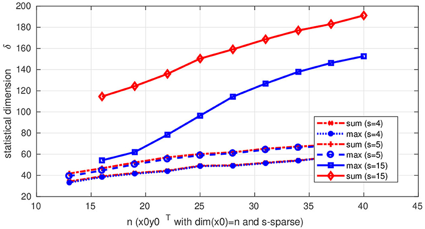
Figure 1. Statistical dimension from (17) for n×n rank-one and s×s–sparse matrices ${𝕄}_{1,s,s}^{n\times n}$ for s = 4, 5, 15, and n ∈ [15, 40]. The results are obtained by averaging the solutions of the corresponding SDP's like e.g., (91) for the sum.

These results indeed suggest that the statistical dimension for optimally weighted maximum of regularizers is better than the sum of regularizers.

3.5.2. Convex Recovery

We numerically find the phase transition for the convex recovery of complex sparse and low-rank matrices using the sum and maximum of optimally weighted ℓ₁ and nuclear norm. We also compare to the results obtained by convex recovery using only either the ℓ₁–norm or the nuclear norm as regularizer and also provide and example for a non-convex algorithm.

The dimension of the matrices are n = n₁ = n₂ = 30, the sparsity range is s = s₁ = s₂ = 5, …, 20, and the rank is r = 1. For each parameter setup a matrix $X_0=u{v}^{†}$ is drawn using a uniform distribution for supports of u and v of size s and iid. standard complex-normal distributed entries on those support. The measurement map itself also consists also of iid. complex-normal distributed entries. The reconstructed vector X is obtained using again the CVX toolbox in MATLAB with the SDPT3 solver and an reconstruction is marked to be successful exactly if

$\begin{array}{ll}{\Vert X-X_0\Vert }_2/\Vert X{\Vert }_2\le 10^{-5}& (92)\end{array}$

holds. Each (m, s)-bin in the phase transition plots contains 20 runs.

The results are shown in Figure 2. Figures 2A,B show the phase transition of only taking the ℓ₁–norm and the nuclear norm as regularizer, respectively. The lower bound from Theorem 5 on the required number of measurements yield for those cases the sparsity s² of X₀ and n, respectively. Thus, only for very small values of s² there is a clear advantage of ℓ₁-regularization compared to the nuclear norm. The actual recovery rates scale roughly as 2s² ln(n² / s²) and 4rn, respectively.

FIGURE 2

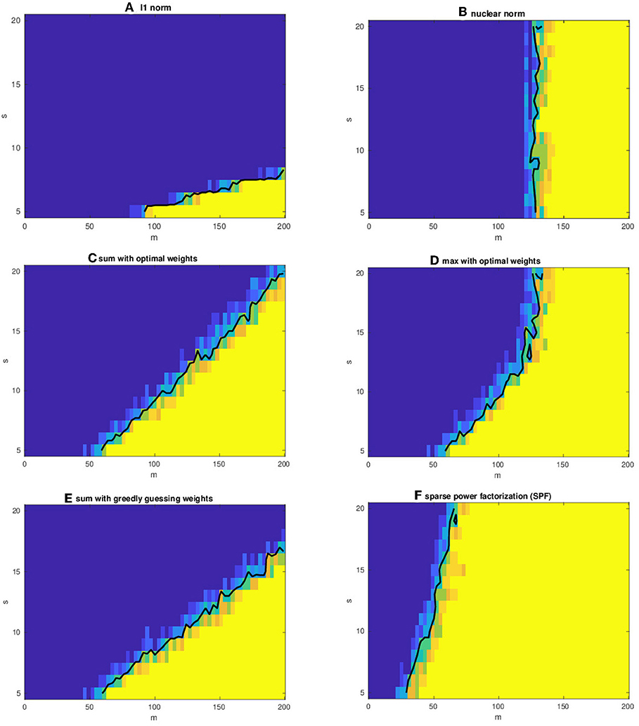
Figure 2. Phase transitions for convex recovery using the ℓ₁–norm (A), nuclear norm (B), the max-norm (D), and the sum-norm (C) with optimal X₀-dependent weights as regularizers. Furthermore, guessing weights in a greedy fashion for the sum-norm using is shown (E) and non-convex recovery using sparse power factorization (SPF) from Lee et al. [22] is in (F). The color indicates the recovery rate with blue encoding 0 and yellow encoding 1.

However, combining both regularizers with optimal weights improves as shown in Figures 2C,D. Both combined approaches instantaneously balance between sparsity and rank. Moreover, there is a clear advantage of taking the maximum (Figure 2C) over of the sum (Figure 2D) of ℓ₁– and nuclear norm. For sufficiently small sparsity the ℓ₁–norm is more dominant and for higher sparsity than the nuclear norm determines the behavior of the phase transition. But only for the maximum of the regularizers the sampling rate saturates at approximately m = 130 due to rank(X₀) = 1 (see Figure 2D).

We also mention that the maximum of regularizers improves only if it is optimally tuned, which is already indicated by the subdifferential of a maximum (12), where only the largest terms contribute. In contrast, reconstruction behavior of the sum of norms seems to more stable. This observations has also been mentioned in Jalali [39]. This feature motivates an empirical approach of guessing the weights from observations.

To sketch a greedy approach for guessing the weights we consider the following strategy. Ideally, we would like to choose λ₁ = 1/∥X₀∥₁ and λ_ℓ1 = 1/∥X₀∥_ℓ1 in the minimization of the objective function λ₁∥X∥₁ + λ_ℓ1∥X∥_ℓ1. Since, for Frobenius norm normalized X we have 1/∥X∥₁ ≥ ∥X∥_∞ (similarly for the ℓ_∞-norm) we choose for as initialization ${\lambda }_1^{(1)}={\parallel {{A}}^{†}(y)\parallel }_{{\ell }_{\infty }}$ and ${\lambda }_{{\ell }_1}^{(1)}={\parallel A^{†}(y)\parallel }_{\infty }$ for the iteration t = 1. After finding

$\begin{array}{ll}{X}^{(t)}≔{arg\; min}_X\left\{{\lambda }_1^{(t)}{\parallel X\parallel }_1+{\lambda }_{{\ell }_1}^{(t)}{\parallel X\parallel }_{{\ell }_1}:{A}(X)=y\right\}& (93)\end{array}$

we update ${\lambda }_1^{(t+1)}≔1/\Vert X^{(t)}{\Vert }_1$ and ${\lambda }_{{\ell }_1}^{(t+1)}≔1/\Vert X^{(t)}{\Vert }_{{\ell }_1}$. The results obtained by this greedy approach after 3 iterations are shown in Figure 2E. Comparing this to the optimally weighted sum of regularizers in Figure 2C, we see that almost the same performance can be achieved with this iterative scheme.

Finally, there is indeed strong evidence that in many problems with simultaneous structures non-convex algorithms perform considerably better and faster then convex ones. Although we have focused in this work on better understand of convex recovery, let us also comment on other settings. For the sparse and low-rank setting there exists several very efficient and powerful algorithms, as examples we mention here sparse power factorization (SPF) [22] and ATLAS_{2, 1} [33]. In the noiseless setting SPF is known to clearly outperforms all convex algorithms (see Figure 2F). The numerical experiments in Fornasier et al. [33] suggests that in the noisy setting ATLAS_{2, 1} seems to be a better choice.

4. Special Low-Rank Tensors

Tensor recovery is an important and notoriously difficult problem, which can be seen as a generalization of low-rank matrix recovery. However, for tensors there are several notions of rank and corresponding tensor decompositions [42]. They include the higher order singular value decomposition (HOSVD), the tensor train (TT) decomposition (a.k.a. by matrix product states), the hierarchical Tucker (a.k.a. tree tensor network) decomposition, and the CP decomposition. For all these notions, the unit rank objects coincide and are given by tensor products.

Gandy et al. [6] suggested to use a sum of nuclear norms of different matrizations (see below) as a regularizer for the completion of 3-way tensors in image recovery problems. Mu et al. [4] showed that this approach leads to the same scaling in the number of required measurements as when one uses just one nuclear norm of one matrization as a regularizer. However, the prefactors are significantly different in these approaches. Moreover, Mu et al. suggested to analyze 4-way tensors, where the matrization can be chosen such that the matrices are close to being square matrices. In this case, the nuclear norm regularization yields an efficient reconstruction method with rigorous guarantees that has the so far best scaling in the number of measurements. For rank-1 tensors we will now suggest to use a maximum of nuclear norms of certain matrizations as a regularizer. While the no-go results [4] for an optimal scaling still hold, this leads to a significant improvement of prefactors.

4.1. Setting and Preliminaries

The effective rank of a matrix X is ${\text{rank}}^{\text{eff}}(X):=\Vert X{\Vert }_1^2/\Vert X{\Vert }_2^2$. Note that for matrices for which all non-zero singular values coincide, the rank coincides with the effective rank and for all other matrices the effective rank is smaller.

We consider the tensor spaces $V≔{ℝ}^{n_1\times n_2\times ···\times n_L}$ as a signal space and refer to the n_i as local dimensions. The different matrix ranks of different matrizations are given as follows.

An index bipartition is

$\begin{array}{ll}\left[L\right]=b\cup b^c\text{ with }b\subset \left[L\right]\text{ and }{b}^c=\left[L\right]\backslash b.& (94)\end{array}$

We call the b-matricization the canonical isomorphism ${𝕂}^{n_1\times n_2\times \dots \times n_L}\cong {𝕂}^{n_b\times n_{b^c}}$, where n_b = ∏_i∈b n_i, i.e., the indices in b are joined together into the row index of a matrix and the indices in b^c into the column index. It is performed by a reshape function in many numerics packages. The rank and effective of the b-matrization of X are denoted by rank_b(X) and ${\text{rank}}_b^{\text{eff}}(X)$. The b-nuclear norm $\parallel X{\parallel }_1^b$ is given by the nuclear norm of the b-matricization of X.

Now, we consider ranks based on a set of index bipartitions

$\begin{array}{ll}{B}={(b_j)}_{j\in \left[k\right]}\text{ with }{b}_j\subset \left[L\right].& (95)\end{array}$

The corresponding (formal) rank ${\text{rank}}_{{B}}$ is given by

$\begin{array}{ll}{\text{rank}}_{{B}}(X)≔{({\text{rank}}_b(X))}_{b\in {B}}& (96)\end{array}$

Similarly, given a signal X₀ ∈ V the corresponding max-norm is given by

$\begin{array}{ll}\begin{array}{c}\parallel X{\parallel }_{{\mu }^{*},max}^B≔\underset{b\in B}{\max }\frac{\parallel X{\parallel }_1^b}{\parallel X_0{\parallel }_1^b}.\end{array}& (97)\end{array}$

Note that for the case that X₀ is a product $X_0=x_0^{(1)}\otimes \dots x_0^{(L)}$ we have

$\begin{array}{ll}\parallel X_0{\parallel }_p^b={\displaystyle \prod _{j=1}^L}{\parallel x_0^{(j)}\parallel }_{{\ell }_2}& (98)\end{array}$

for all b ⊂ [L] and p ≥ 1. Hence, the reweighting in the optimal max-norm (97) is trivial in that case, i.e., it just yields an overall factor, which can be pulled out of the maximum.

Let us give more explicit examples for the set of bipartitions: ${B}={(\left\{i\right\})}_{i\in \left[L\right]}$ defines the HOSVD rank and ${B}={(\left\{1,\dots ,\ell \right\})}_{\ell \in \left[L-1\right]}$ the tensor train rank. They also come along with a corresponding tensor decomposition. In other cases, accompanying tensor decompositions are not known. For instance, for k = 4 and ${B}=(\left\{1,2\right\},\left\{1,3\right\})$ it is clear that the tensors of (formal) rank (1, 1) are tensor products. The tensors of ranks (1, i) and (i, 1) are given by tensor products of two matrices, each of rank bounded by i. But in general, it is unclear what tensor decomposition corresponds to a ${B}$-rank.

One interesting remark might be that there are several measures of entanglement in quantum physics, which measure the non-productness in case of quantum state vectors. The negativity [43] is such a measure. Now, for a non-trivial bipartition b and normalized tensor X ∈ V (i.e., ∥X∥_ℓ2 = 1)

$\begin{array}{ll}\frac{1}{2}\left({\left({\Vert X\Vert }_1^b\right)}^2-1\right)=\frac{1}{2}\left({\Vert {(\text{vec}(X) \text{vec}{(X)}^T)}^{T_b}\Vert }_1-1\right)& (99)\end{array}$

is the negativity [43] of the quantum state vector X w.r.t. the bipartition b, where T_b denotes the partial transposition w.r.t. b and vec(X) the vectorization of X, i.e., the [L]-matrization.

Theorem 5 applies to tensor recovery with the regularizer (97). We illustrate the lower bound for the special case of 4-way tensors (L = 4) with equal local dimensions n_i = n and a regularizer norm given by ${B}=(\{1,2\},\{1,3\},\{1,4\})$. Then the critical number of measurements (45) in the lower bounds (46) and (43) is

$\begin{array}{ll}\kappa =\delta (D({\parallel ·\parallel }_{{\mu }^{*},\text{max}};x_0))\approx {\displaystyle \underset{b\in {B}}{min}}{\text{rank}}_b^{\text{eff}}(X_0)n^2.& (100)\end{array}$

If X₀ is a tensor product, this becomes κ ≈ n².

4.2. RIP for the HOSVD and TT Ranks

A similar statement as Theorem 7 has been proved for the HOSVD and TT rank for the case of sub-Gaussian measurements by Rauhut et al. [44, section 4]. They also showed that the RIP statements lead to a partial recovery guarantee for iterative hard thresholding algorithms. Having only suboptimal bounds for TT and HOSVD approximations has so far prevented proofs of full recovery guarantees.

It is unclear how RIP results could be extended to the “ranks” without an associated tensor decomposition and probably these ranks need to be better understood first.

4.3. Numerical Experiments

We sample the statistical dimension (17) numerically for L = 4 instances of the max-norm (97) and a unit rank signal X₀; see Figure 3, where we have estimated the statistical dimension using the program (64) with the dual norms being spectral norms of the corresponding b-matrizations. The numerical experiments suggest that the actual reconstruction behavior of the ${{B}}_3$-max-norm is close to twice the lower bound from Theorem 5, which is given by n². The missing factor of two might be due to the following mismatch. In the argument with the circular cones we only considered tensors of unit b-rank whereas the actual descent cone contains tensors of b-rank 2 for some $b\in {{B}}_3$. This discrepancy should lead to the lower bound be too low by a factor of 2 which is compatible with the plots in Figure 3.

FIGURE 3

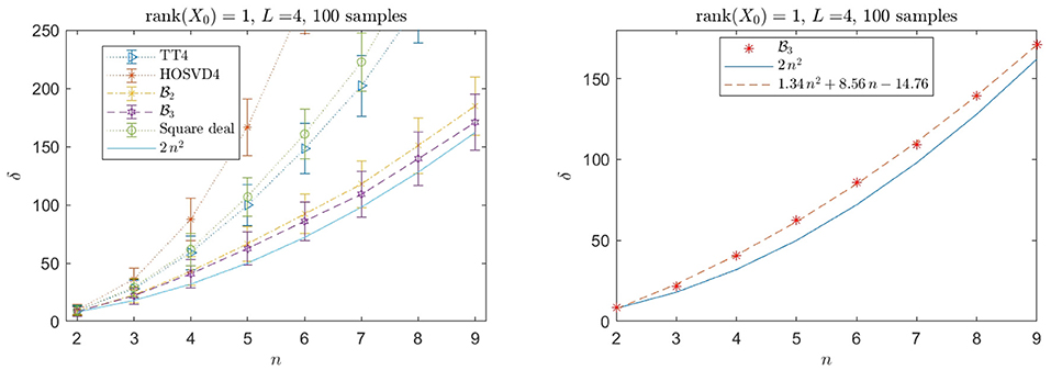
Figure 3. Observed average of the statistical dimension (17) for a product signal $X_0\in {({ℂ}^n)}^{\otimes k}$ with L = 4 and the max-norm (97) as regularizer. The norm is given by the bipartitions corresponding to (i) the TT decomposition, (ii) the HOSVD decomposition, (iii) ${{B}}_2≔(\left\{1,2\right\},\left\{1,3\right\})$, ${{B}}_3≔(\left\{1,2\right\},\left\{1,3\right\},\left\{1,4\right\})$, and ${{B}}_{\text{Square deal}}≔(\left\{1,2\right\})$. The statistical dimension δ corresponds to the critical number of measurements where the phase transition in the reconstruction success probability occurs. The plots suggest that for the ${{B}}_3$-max-norm the number of measurements scales roughly as twice the lower bound given by (100). For the numerical implementation, the SDP (64) has been used. The error bars indicate the unbiased sample standard deviation. The numerics has been implemented with Matlab+CVX+SDPT3.

A similar experiment can be done for the related sum-norm from (18). This leads to similar statistical dimensions except for the tensor train bipartition, where the statistical dimension is significantly larger (~ 25%) for the sum-norm.

5. Conclusion and Outlook

We have investigated the problem of convex recovery of simultaneously structured objects from few random observations. We have revisited the idea of taking convex combinations of regularizers and have focused on the best among them, which is given by an optimally weighted maximum of the individual regularizers. We have extended lower bounds on the required number of measurements by Mu et al. [4] to this setting. The bounds are simpler and more explicit than those obtained by Oymak et al. [5] for simultaneously low rank and sparse matrices. They show that it is not possible to improve the scaling of the optimal sampling rate in convex recovery even if optimal tuning and the maximum of simultaneous regularizers are used, the latter giving the largest subdifferential. In more detail, we have obtained lower bounds for the number of measurements in the generic situation and applied this to the cases of (i) simultaneously sparse and low-rank matrices and (ii) certain tensor structures.

For these settings, we have compared the lower bounds to numerical experiments. In those experiments we have (i) demonstrated the actual recovery and (ii) estimated the statistical dimension that gives the actual value of the phase transition of the recovery rate. The latter can be achieved by sampling over certain SDPs. For tensors, we have observed that the lower bound can be quite tight up to a factor of 2.

The main question, whether or not one can derive strong rigorous recovery guarantees for efficient reconstruction algorithms in the case of simultaneous structures remains largely open. However, there are a few smaller questions that we would like to point out.

Numerically, we have observed that weights deviating from the optimal ones have a relatively small effect for the sum of norms as compared to the maximum of norms. Indeed, $\delta (\mu ):=\delta \left(\text{cone}{(\partial {\Vert \cdot \Vert }_{\text{λ,sum}}(x_0))}^{\circ }\right)$ is a continuous function of μ whereas it appears to be non-continuous for $\parallel ·\parallel$_μ,max due to (13). Of course it would be good to have tight upper bounds both regularizers. Perhaps, one can also find a useful interpolation between $\parallel ·\parallel$_μ,sum and $\parallel ·\parallel$_μ,max by using an ℓ_p norm of the vector containing the single norms ${\mu }_i^{*}{\Vert \cdot \Vert }_{(i)}$. This interpolation would give the max-norm $\parallel ·\parallel$_μ,max for p = ∞ and the sum-norm $\parallel ·\parallel$_μ,sum for p = 1 and one could choose p depending on how accurately one knows the optimal weights μ^*. Finally, perhaps one can modify an iterative non-convex procedure for solving the optimization problem we are using for the reconstructions such that one obtains recovery from fewer measurements.

Author Contributions

All authors listed have made a substantial, direct and intellectual contribution to the work, and approved it for publication.

Funding

The work of MK was funded by the National Science Centre, Poland within the project Polonez (2015/19/P/ST2/03001) which has received funding from the European Union's Horizon 2020 research and innovation programme under the Marie Skłodowska-Curie grant agreement No 665778. The work of SS was partially supported by the grant DMS-1600124 from the National Science Foundation (USA). PJ was supported by DFG grant JU 2795/3. Moreover, we acknowledge support by the German Research Foundation and the Open Access Publication Fund of the TU Berlin.

Conflict of Interest Statement

The authors declare that the research was conducted in the absence of any commercial or financial relationships that could be construed as a potential conflict of interest.

Acknowledgments

We thank Michał Horodecki, Omer Sakarya, David Gross, Ingo Roth, Dominik Stoeger, and Željka Stojanak for fruitful discussions.

Footnotes

1. ^See the cited works for further references on the classical non-sparse phase retrieval problem.

2. ^Assuming that k₁ ≔ rs₁ ≤ n₁ and k₂ ≔ rs₂ ≤ n₂.

References

1. Foucart S, Rauhut H. A Mathematical Introduction to Compressive Sensing. New York, NY: Springer (2013).

Google Scholar

2. Chandrasekaran V, Recht B, Parillo A, Willsky AS. The convex geometry of linear inverse problems. Found Comput Math. (2012) 12:805–49. doi: 10.1007/s10208-012-9135-7

CrossRef Full Text | Google Scholar

3. Amelunxen D, Lotz M, McCoy MB, Tropp JA. Living on the edge: phase transitions in convex programs with random data. Inform Infer. (2014) 3:224–94. doi: 10.1093/imaiai/iau005

CrossRef Full Text | Google Scholar

4. Mu C, Huang B, Wright J, Goldfarb D. Square deal: lower bounds and improved relaxations for tensor recovery. In: Proceedings of the 31st International Conference on Machine Learning. Beijing (2013).

Google Scholar

5. Oymak S, Jalali A, Fazel M, Eldar YC, Hassibi B. Simultaneously structured models with application to sparse and low-rank matrices. IEEE Trans. Inf. Theory (2015) 61:2886–908. doi: 10.1109/TIT.2015.2401574

CrossRef Full Text | Google Scholar

6. Gandy S, Recht B, Yamada I. Tensor completion and low-n-rank tensor recovery via convex optimization. Inverse Probl. (2011) 27:025010. doi: 10.1088/0266-5611/27/2/025010

CrossRef Full Text | Google Scholar

7. Ghadermarzy N, Plan Y, Yilmaz Ö. Near-optimal sample complexity for convex tensor completion. Inform Infer. (2017) iay019. doi: 10.1093/imaiai/iay019

CrossRef Full Text | Google Scholar

8. Rauhut H, Stojanac Ž. Tensor theta norms and low rank recovery. arXiv:1505.05175. (2015).

Google Scholar

9. Richard E, Obozinski GR, Vert JP. Tight convex relaxations for sparse matrix factorization. In: Z Ghahramani, M Welling, C Cortes, ND Lawrence, and KQ Weinberger editors. Advances in Neural Information Processing Systems 27. Montréal, QC: Curran Associates, Inc. (2014). p. 3284–92.

Google Scholar

10. Tropp JA. Convex recovery of a structured signal from independent random linear measurements. In: Pfander G, editor. Sampling Theory, a Renaissance. Applied and Numerical Harmonic Analysis. Cham: Birkhäuser (2014). p. 67–101.

Google Scholar

11. Hiriart-Urruty JB, Lemaréchal C. Fundamentals of Convex Analysis. Grundlehren text editions. Berlin; New York, NY: Springer (2001).

Google Scholar

12. Amelunxen D, Lotz M, McCoy MB, Tropp JA. Living on the edge: phase transitions in convex programs with random data. arXiv:1303.6672v2 (2013).

Google Scholar

13. Doan XV, Vavasis S. Finding approximately rank-one submatrices with the nuclear norm and ℓ₁-Norm. SIAM J Optim. (2013) 23:2502–40. doi: 10.1137/100814251

CrossRef Full Text | Google Scholar

14. Rockafellar R. Convex Analysis. Princeton, NJ: Princeton University Press (1970). Second printing (1972).

Google Scholar

15. Kliesch M, Szarek SJ, Jung P. Simultaneous structures in convex signal recovery - revisiting the convex combination of norms. arXiv:1904.07893. (2019).

Google Scholar

16. [Dataset] Dual of the Minkowski Sum,. Available onlie at: http://math.stackexchange.com/questions/1766775/dual-of-the-minkowski-sum (2016). (accessed February 15, 2017).

17. Li X, Voroninski V. Sparse signal recovery from quadratic measurements via convex programming. SIAM J. Math. Anal. (2013) 45:3019–33. doi: 10.1137/120893707

CrossRef Full Text | Google Scholar

18. Jaganathan K, Oymak S, Hassibi B. Sparse phase retrieval: convex algorithms and limitations. In: 2013 IEEE International Symposium on Information Theory Proceedings (ISIT). Istanbul (2013). doi: 10.1109/ISIT.2013.6620381

CrossRef Full Text | Google Scholar

19. Rubinstein R, Zibulevsky M, Elad M. Double sparsity: learning sparse dictionaries for sparse signal approximation. IEEE Trans. Signal Process. (2010) 58:1553–64. doi: 10.1109/TSP.2009.2036477

CrossRef Full Text | Google Scholar

20. Smola AJ, Schölkopf B. Sparse greedy matrix approximation for machine learning. In: Proceedings of the Seventeenth International Conference on Machine Learning. San Francisco, CA (2000). p. 911–8.

Google Scholar

21. Johnstone IM, Lu AY. On consistency and sparsity for principal components analysis in high dimensions. J Am Stat Assoc. (2009) 104:682–93. doi: 10.1198/jasa.2009.0121

PubMed Abstract | CrossRef Full Text | Google Scholar

22. Lee K, Wu Y, Bresler Y. Near optimal compressed sensing of sparse rank-one matrices via sparse power factorization. IEEE Trans Inform Theor. (2013) 64:1666-98. doi: 10.1109/TIT.2017.2784479

CrossRef Full Text | Google Scholar

23. Lee K, Li Y, Junge M, Bresler Y. Blind recovery of sparse signals from subsampled convolution. IEEE Trans Inform Theor. (2017) 63:802–21. doi: 10.1109/TIT.2016.2636204

CrossRef Full Text | Google Scholar

24. Flinth A. Sparse blind deconvolution and demixing through ℓ_1, 2-minimization. Adv Comput Math. (2018) 44:1–21. doi: 10.1007/s10444-017-9533-0

CrossRef Full Text | Google Scholar

25. Lee K, Li Y, Junge M, Bresler Y. Stability in blind deconvolution of sparse signals and reconstruction by alternating minimization. In: 2015 International Conference on Sampling Theory and Applications, SampTA 2015. Washington, DC (2015). p. 158–62. doi: 10.1109/SAMPTA.2015.7148871

CrossRef Full Text | Google Scholar

26. Aghasi A, Ahmed A, Hand P. BranchHull: convex bilinear inversion from the entrywise product of signals with known signs. Appl Comput Harmon Anal. (2017). doi: 10.1016/j.acha.2019.03.002

CrossRef Full Text | Google Scholar

27. Geppert J, Krahmer F, Stöger D. Sparse power factorization: balancing peakiness and sample complexity. In: 2018 IEEE Statistical Signal Processing Workshop (SSP). Freiburg (2018).

Google Scholar

28. Ling S, Strohmer T. Self-calibration and biconvex compressive sensing. Inverse Probl. (2015) 31:115002. doi: 10.1088/0266-5611/31/11/115002

CrossRef Full Text | Google Scholar

29. Jung P, Walk P. Sparse model uncertainties in compressed sensing with application to convolutions and sporadic communication. In: Boche H, Calderbank R, Kutyniok G, Vybiral J, editors. Compressed Sensing and its Applications. (Cham: Springer) (2015). p. 1–29. doi: 10.1007/978-3-319-16042-9_10

CrossRef Full Text

30. Wunder G, Boche H, Strohmer T, Jung P. Sparse signal processing concepts for efficient 5g system design. IEEE Access. (2015) 3:195–208. doi: 10.1109/ACCESS.2015.2407194

CrossRef Full Text | Google Scholar

31. Roth I, Kliesch M, Wunder G, Eisert J. Reliable recovery of hierarchically sparse signals and application in machine-type communications. arXiv:1612.07806. (2016).

Google Scholar

32. Berthet Q, Rigollet P. Complexity theoretic lower bounds for sparse principal component detection. JMLR (2013) 30:1–21. doi: 10.1109/ICEEI.2011.6021515

CrossRef Full Text | Google Scholar

33. Fornasier M, Maly J, Naumova V. Sparse PCA from inaccurate and incomplete measurements. arXiv:1801.06240. (2018).

Google Scholar

34. Baraniuk R, Davenport M, DeVore R, Wakin M. A simple proof of the restricted isometry property for random matrices. Construct Approx. (2008) 28:253–63. doi: 10.1007/s00365-007-9003-x

CrossRef Full Text | Google Scholar

35. Candes E, Plan Y. Tight oracle inequalities for low-rank matrix recovery from a minimal number of noisy random measurements. IEEE Trans Inf Theory. (2011) 57:2342–359. doi: 10.1109/TIT.2011.2111771

CrossRef Full Text | Google Scholar

36. Recht B, Fazel M, Parrilo P. Guaranteed minimum-rank solutions of linear matrix equations via nuclear norm minimization. SIAM Rev. (2010) 52:471–501. doi: 10.1137/070697835

CrossRef Full Text | Google Scholar

37. Candes EJ, Tao T. Decoding by linear programming. IEEE Trans Inf Theory. (2005) 51:4203–15. doi: 10.1109/TIT.2005.858979

CrossRef Full Text | Google Scholar

38. Gross D. Recovering low-rank matrices from few coefficients in any basis. IEEE Trans Inf Theory. (2011) 57:1548–66. doi: 10.1109/TIT.2011.2104999

CrossRef Full Text | Google Scholar

39. Jalali A. Convex Optimization Algorithms and Statistical Bounds for Learning Structured Models. Ph.D. thesis, University of Washington, Seattle, WA (2016).

Google Scholar

40. Foucart S, Gribonval R, Jacques L, Rauhut H. Jointly low-rank and bisparse recovery: Questions and partial answers. ArXiv-preprint. (2019) arxiv:1902.04731.

Google Scholar

41. Iwen M, Viswanathan A, Wang Y. Robust sparse phase retrieval made easy. Applied and Computational Harmonic Analysis 42 (2017) 135–142. doi: 10.1016/j.acha.2015.06.007

CrossRef Full Text | Google Scholar

42. Kolda T, Bader B. Tensor decompositions and applications. SIAM Rev. (2009) 51:455–500. doi: 10.1137/07070111X.

CrossRef Full Text | Google Scholar

43. Vidal G, Werner RF. Computable measure of entanglement. Phys Rev A. (2002) 65:032314. doi: 10.1103/PhysRevA.65.032314

CrossRef Full Text | Google Scholar

44. Rauhut H, Schneider R, Stojanac Z. Low rank tensor recovery via iterative hard thresholding. Linear Algebra and its Applications (2016) 523:220–62. doi: 10.1016/j.laa.2017.02.028

CrossRef Full Text | Google Scholar