Least Square Approach to Out-of-Sample Extensions of Diffusion Maps

1. Introduction

Recently, in many scientific and technological areas, we need to analyze and process high-dimensional data, such as speech signals, images and videos, text documents, stock trade records, and others. Due to the curse of dimensionality [1, 2], directly analyzing and processing high-dimensional data are often infeasible. Therefore, dimensionality reduction (DR) (see the books [3, 4]) becomes a critical step in high-dimensional data processing. DR maps high-dimensional data into a low-dimensional space so that the data process can be carried out on its low-dimensional representation. There exist many DR methods in literature. The famous linear method is principle component analysis (PCA) [5]. However, PCA cannot effectively reduce the dimension for the data set, which essentially resides on a nonlinear manifold. Therefore, to reduce the dimensions of such data sets, people employ non-linear DR methods [6–12], among which, the method of Diffusion Maps (Dmaps) introduced by Coifman and his research group [13, 14] have been proved attractive and effective. Adopting the ideas of the spectral clustering [15, 16] and Laplacian eigenmaps [17], Dmaps integrates them into a more conceptual framework—the geometric harmonics.

As a spectral method, Dmaps employs the diffusion kernel to define the similarity on a given data set X ⊂ ℝ^D. The principal d-dimensional eigenspace (d ≪ D) of the kernel provides the feature space of X, so that a diffusing mapping 𝔉 maps X to the set Y = 𝔉(X), which is called a DR of X.

Note that the mapping 𝔉 is constructed by the spectral decomposition of the kernel, which is data-dependent. If the set X is enlarged to X = X ∪ Z and we want to make DR of X by Dmaps, we have to retrain the set X in order to construct a new diffusing mapping. The retraining approach is often unpractical if the cardinality of X becomes very large, or the new data set Z comes as a time-stream.

Out-of-example DR extension method finds the DR of X by extending the diffusing mapping 𝔉 onto X. In most cases, we can assume that the new data set Z has the similar features as X. Therefore, instead of retraining the whole set X, we realize the DR of X by extending the mapping 𝔉 from X to X only.

Lots of papers have introduced various out-of-example extension algorithms (see [14, 18, 19] and their references). However, the mathematical analysis on out-of-example extension is not studied sufficiently.

The main purpose of this paper is to give a mathematical analysis on the out-of-sample DR extension of Dmaps. In Wang [20], we preliminarily studied out-of-sample DR extensions for kernel PCA. Since the structure of kernels for Dmaps are different from kernel PCA, it needs a special analysis. In this paper we deal with the DR extensions of Dmaps in the framework of reproducing kernel Hilbert space (RKHS), in which Dmaps extension can be classified as the least square one.

The paper is organized as follows: In section 2, we introduce the general out-of-sample extensions in the RKHS framework. In section 3, we establish the least square out-of-sample DR extensions of Dmaps. In section 4, we give the mathematical analysis and algorithms for the Dmaps DR extension. In the last section, we give several examples for the extension.

2. Preliminary

We first introduce some notions and notations. Let μ be a finite (positive) measure on a data set X ⊂ ℝ^D. We denoted by L²(X, μ) the (real) Hilbert space on X, equipped with the inner product

$\begin{array}{l}{\langle f,g\rangle }_{L^2(X,\mu )}={\displaystyle {\int }_X}f(x)g(x)d\mu (x),f,g\in L^2(X,\mu ).\end{array}$

Then, $\left|\right|f|{|}_{L^2(X,\mu )}=\sqrt{{\langle f,f\rangle }_{L^2(X,\mu )}}$. Later, we will abbreviate L²(X, μ) to L²(X) (or L²) if the measure μ (and the set X) is (are) not stressed.

Definition 1 A function k: X² → ℝ is called a Mercer's kernel if it satisfies the following conditions:

1. k is symmetric: k(x, y) = k(y, x);

2. k is positive semi-definite;

3. k is bounded on X², that is, there is an M > 0 such that |k(x, y)| ≤ M, (x, y) ∈ X².

In this paper, we only consider Mercer's kernels. Hence, the term kernel will stand for Mercer's one. The kernel distance (associated with k) between two points x, y ∈ X is defined by

$\begin{array}{l}{d}_k(x,y)=\sqrt{k(x,x)+k(y,y)-2k(x,y)}.\end{array}$

A kernel k defines an RKHS H_k, in which the inner product satisfies [21]

$\begin{array}{ll}{\langle f(·),k(x,·)\rangle }_{H_k}=f(x),f\in H_k,x\in X.& (1)\end{array}$

Later, we will use H instead of H_k if the kernel k is not stressed. Recall that k has a dual identity. It derives the identity operator on H, as shown in 1, and also derives the following compact operator K on L²(X):

$\begin{array}{l}(Kf)(x)={\langle f(·),k(x,·)\rangle }_{L^2}={\displaystyle {\int }_X}k(x,y)f(y)d\mu (y),f\in L^2.\end{array}$

In Wang [20], we proved that if

$\begin{array}{l}k(x,y)={\displaystyle \sum _{j=1}^m}{\varphi }_j(x){\varphi }_j(y),\end{array}$

where the set {ϕ₁, ··· , ϕ_m} is linearly independent, then the set is an o.n. basis of H. Therefore, for f, g ∈ H with $f=\sum _j{c}_j{\varphi }_j$ and $g=\sum _j{d}_j{\varphi }_j$, we have ${\langle f,g\rangle }_{H_k}=\sum _j{c}_j{d}_j$.

Let the spectral decomposition of k be the following:

$\begin{array}{ll}k(x,y)={\displaystyle \sum _{j=1}^m}{\lambda }_j{v}_j(x)v_j(y),0\le m\le \infty ,& (2)\end{array}$

where the eigenvalues are arranged decreasingly, λ₁ ≥ ··· ≥ λ_m > 0, and the eigenfunctions v₁, v₁, ··· , v_m, are normalized to satisfy

$\begin{array}{l}{\langle v_i,v_j\rangle }_{L^2(X)}={\delta }_{i,j}.\end{array}$

Write ${\gamma }_i(x)=\sqrt{{\lambda }_i}{v}_i(x)$. Then, {γ₁, ··· , γ_m} is an o.n. basis of H, which is called the canonic basis of H. We also call $k(x,y)=\sum _{j=1}^m{\gamma }_j(x){\gamma }_j(y)$ the canonic decomposition of k. By 2, we have

$\begin{array}{l}{\gamma }_j=\frac{1}{{\lambda }_j}{\displaystyle {\int }_X}k(x,y){\gamma }_j(y)d\mu (y).\end{array}$

Thus, if f ∈ H have the canonic representation $f=\sum _{j=1}^m{c}_j{\gamma }_j$, then, for any g ∈ H, the inner product 〈f, g〉_H has the following integral form:

$\begin{array}{l}{\langle f,g\rangle }_H={\displaystyle \sum _{j=1}^m}\frac{c_j}{{\lambda }_j}{\displaystyle {\int }_X}g(x){\gamma }_j(x)d\mu (x).\end{array}$

To investigate the out-of-sample DR extension, we first recall some general results on function extensions. Let X = X ∪ Z. To stress that a point x ∈ X is also in X, we use x instead of x. Similarly, we denote by k(x, y) the restriction of k(x, y) on X². That is,

$\begin{array}{l}k(x,y)=\text{k}(\text{x},\text{y}),(\text{x},\text{y})\in {\text{X}}^2.\end{array}$

We also denote by H the RKHS associated with k. Then a continuous map E : H → H is called an extension if

$E(f)(x)=f(x),\forall f\in H.$

Correspondingly, we define the restriction R: H → H by

$\begin{array}{l}R(f)(\text{x})=f(\text{x}),\forall f\in H,\text{x}\in \text{X}.\end{array}$

It is obvious that the extensions from X to X are not unique if Z is not empty. So, we define the set of all extensions of f ∈ H by

$\begin{array}{l}{A}_{\text{f}}=\left\{f\in H;R(f)=\text{f}\right\},\end{array}$

and call $\widehat{f}\in A_{\text{f}}$ the least-square extension of f if

$\begin{array}{l}\left|\right|\widehat{f}|{|}_H={\displaystyle \underset{f\in A_{\text{f}}}{min}}|\left|f\right|{|}_H.\end{array}$

It is evident that the least-square extension of a function is unique. We denote by T : H → H the operator of the least-square extension.

In Wang [20], we already prove the following:

1. Let {v₁, ··· , v_d} be the canonic basis of H and σ₁ ≥ σ₂ ≥ ··· ≥ σ_d > 0 be the eigenvalues of the kernel k(x, y). Then the least-square extension of v_j is

$\begin{array}{ll}{\widehat{v}}_j(x)(=\text{T}({\text{v}}_j)(x))=\frac{1}{{\sigma }_j}{\displaystyle {\int }_{\text{X}}}k(x,\text{y}){\text{v}}_j(\text{y})d\mu (\text{y}),x\in X,1\le j\le d.& (3)\end{array}$

Therefore, for any $\text{f}=\sum _{j=1}^d{c}_j{\text{v}}_j\in \text{H}$,

$\begin{array}{l}\widehat{f}(x)(=\text{T}(\text{f})(x))={\displaystyle \sum _{j=1}^d}{c}_j\frac{1}{{\sigma }_j}{\displaystyle {\int }_{\text{X}}}k(x,\text{y}){\text{v}}_j(\text{y})d\mu (\text{y}).\end{array}$

2. Let Ĥ = T(H) and T* : H → H be the joint operator of T. Then P = TT* is an orthogonal projection from H to Ĥ.

3. Let $\widehat{k}(x,y)$ be the kernel of the RKHS Ĥ. Then $k_0(x,y)=k(x,y)-\widehat{k}(x,y)$ is a Mercer's kernel such that $k_0(x,y)=0,(x,y)\in X^2\backslash {\text{X}}^2$. Denote by H₀ the RKHS associated with k₀. Then, H = Ĥ ⊕ H₀ and Ĥ ⊥ H₀.

4. If k(x, y) is a Gramian-type DR kernel [20], and ${\left[{\text{v}}_1(\text{X}),···,{\text{v}}_d(\text{X})\right]}^T$ gives the DR of X, then ${\left[{\widehat{v}}_1(X),···,{\widehat{v}}_d(X)\right]}^T$ provides the least-square out-of-sample DR extension on X.

3. Least-Square Out-of-Sample DR Extensions for Dmaps

The kernels of Dmaps are constructed based on the Gaussian kernel

$\begin{array}{l}w(x,y)=exp\left(-\frac{\left|\right|x-y|{|}^2}{ϵ}\right),(x,y)\in X^2,ϵ>0.\end{array}$

The function

$\begin{array}{l}S(x)={\displaystyle {\int }_X}w(x,y)d\mu (y)\end{array}$

defines a mass density on X, and $M={\int }_{X}S(x)d\mu (x)$ is the total mass of X.

There are two important forms of the kernels of Dmaps: The Graph-Laplacian diffusion kernel and the Laplace-Beltrami one.

3.1. Dmaps With the Graph-Laplacian Kernel

We first discuss the least-square out-of-sample DR Extensions for the Dmaps with the Graph-Laplacian (GL) kernel. Normalizing the Gaussian kernel by S(x), we obtain the following Graph-Laplacian diffusion kernel [4, 13]:

$\begin{array}{l}g(x,y)=\frac{w(x,y)}{\sqrt{S(x)S(y)}}.\end{array}$

This kernel relates to the data set X equipped with an undirected (weighted) graph. It is known that 1 is the greatest eigenvalue of g(x, y) and its corresponding normalized eigenfunction is $\sqrt{\frac{S(x)}{M}}$.

Let H_g be the RKHS associated with the kernel g and {ϕ₀, ··· , ϕ_m} be its canonic basis, which suggest the following spectral decomposition of g(x, y):

$\begin{array}{l}g(x,y)={\displaystyle \sum _{j=0}^m}{\lambda }_j{v}_j(x)v_j(y),\end{array}$

where 1 = λ₀ ≥ λ₁ ≥ ··· ≥ λ_m > 0 and $v_j(x)={\varphi }_j(x)/\sqrt{{\lambda }_j}$. Because ${\varphi }_0=\sqrt{\frac{S(x)}{M}}$ provides only the mass information of the data set, it should not reside on the feature space. Hence, we define the feature space as the RKHS associated with the kernel $\sum _{j=1}^m{\varphi }_j(x){\varphi }_j(y)$, where ϕ₀ is removed.

Definition 2. The mapping $\Phi :X\to {ℝ}^m:\Phi (x)={\left[{\varphi }_1(x),···,{\varphi }_m(x)\right]}^T$ is called the diffusion mapping and the data set Φ(X) ⊂ ℝ^m is called a DR of X.

Remark. In Wang [20], we already pointed out that each orthogonal transformation of the set Φ(X) can also be considered as a DR of X. Hence, any non-canonical o.n. basis of the feature space also provides a DR mapping.

To study the out-of-sample extension, as what was done in the preceding section, we assume X = X ∪ Z and denote by g(x, y) the Graph-Laplacian kernel on X, that is,

$\begin{array}{l}\text{g}(\text{x},\text{y})=\frac{\text{w}(\text{x},\text{y})}{\sqrt{\text{S}(\text{x})\text{S}(\text{y})}},\end{array}$

where S(x) is the mass density on X, and

$\begin{array}{l}\text{w}(\text{x},\text{y})=w(\text{x},\text{y}),(\text{x},\text{y})\in {\text{X}}^2,\end{array}$

Assume that spectral decomposition of g is given by

$\begin{array}{ll}\text{g}(\text{x},\text{y})={\displaystyle \sum _{j=0}^d}{\sigma }_j{\text{v}}_j(\text{x}){\text{v}}_j(\text{y}).& (4)\end{array}$

Then the RKHS H_g associated with g has the canonic basis {φ₀, φ₁, ··· , φ_d}:

$\begin{array}{l}\text{g}(\text{x},\text{y})={\displaystyle \sum _{j=0}^d}{\phi }_j(\text{x}){\phi }_j(\text{y}),\end{array}$

where ${\phi }_j=\sqrt{{\sigma }_j}{\text{v}}_j$. Because S(x) ≠ S(x), in general,

$\begin{array}{l}\text{g}(\text{x},\text{y})\ne g(\text{x},\text{y}),(\text{x},\text{y})\in {\text{X}}^2.\end{array}$

Hence, we cannot directly apply the extension technique in the preceding section to g. Our main purpose in this subsection is to introduce the extension from H_g to H_g.

Denote by H_w and H_w the RKHSs associated with the kernels w and w, respectively. Because w(x, y) = w(x, y) for (x, y) ∈ X², the extension technique in the preceding section can be applied.

Let ${\text{u}}_j(\text{x})=\sqrt{\text{S}(\text{x})}{\phi }_j(\text{x})$ and $u_j(x)=\sqrt{S(x)}{\varphi }_j(x)$. Then we have

$\begin{array}{l}\text{w}(\text{x},\text{y})={\displaystyle \sum _{j=0}^d}{\text{u}}_j(\text{x}){\text{u}}_j(\text{y}),w(x,y)={\displaystyle \sum _{j=0}^m}{u}_j(x)u_j(y).\end{array}$

Lemma 3 The least-square extension operator T : H_w → H_w has the following representation:

$\begin{array}{ll}\text{T}({\text{u}}_j)(x)=\frac{1}{{\sigma }_j}{\displaystyle {\int }_{\text{X}}}w(x,\text{y})\frac{{\text{u}}_j(\text{y})}{\text{S}(\text{y})}d\mu (\text{y}),j=0,1,···,d.& (5)\end{array}$

Proof. Because ${\left\{{\text{u}}_j\right\}}_{j=0}^d$ is not a canonic o.n. basis of H_w, we cannot directly apply the extension formula 3. Recall that the formula 3 can also be written as T(f)(x) = 〈f, k(x, ·)〉_H. (In the considered case, the kernel w replaces k.) Note that

$\begin{array}{l}{\langle {\text{u}}_j,\text{w}(\text{x},·)\rangle }_{H_{\text{w}}}={\text{u}}_j(\text{x})=\sqrt{\text{S}(\text{x})}{\phi }_j(\text{x})=\sqrt{\text{S}(\text{x})}\frac{1}{{\sigma }_j}{\displaystyle {\int }_{\text{X}}}\text{g}(\text{x},\text{y}){\phi }_j(\text{y})\\ d\mu (\text{y})=\frac{1}{{\sigma }_j}{\displaystyle {\int }_{\text{X}}}\text{w}(\text{x},\text{y})\frac{{\text{u}}_j(\text{y})}{\text{S}(\text{y})}d\mu (\text{y}),\end{array}$

which implies that, for any f ∈ H_w, we have

$\begin{array}{l}{\langle \text{f},{\text{u}}_j\rangle }_{H_{\text{w}}}=\frac{1}{{\sigma }_j}{\displaystyle {\int }_{\text{X}}}\text{f}(\text{y})\frac{{\text{u}}_j(\text{y})}{\text{S}(\text{y})}d\mu (\text{y}).\end{array}$

Therefore, the formula T(u_j)(x) = 〈w(x, ·),_uj〉Hw yields 5. ■

We now write û_j = T(u_j) and define

$\begin{array}{l}ŵ(x,y)={\displaystyle \sum _{j=0}^d}{û}_j(x){û}_j(y).\end{array}$

Then the RKHS H_ŵ associated with the kernel ŵ is the extension of H_w.

The function S(x) induces the following multiplicator from H_g to H_w:

$\begin{array}{l}{𝔖}_S(f)(x)=\sqrt{S(x)}f(x),x\in X.\end{array}$

Similarly, the function S(x) induces the following multiplicator from H_g to H_w:

$\begin{array}{l}{𝔖}_{\text{S}}(\text{f})(\text{x})=\sqrt{\text{S}(\text{x})}\text{f}(\text{x}),\text{x}\in \text{X}.\end{array}$

It is clear that the operator 𝔖_S (𝔖_S) is an isometric mapping. With the aid of 𝔖_S and 𝔖_S, we define the least-square extension ${T}$ from H_g to H_g by

$\begin{array}{ll}T={({𝔖}_S)}^{-1}\circ \text{T}\circ {𝔖}_{\text{S}}.& (6)\end{array}$

The following diagram shows the strategy of the out-of-sample extension using Graph-Laplacian diffusion mapping.

We now derive the integral representation of the operator ${T}$.

Lemma 4 Let the canonic decomposition of g be given by 4 and $\text{f}=\sum _{j=0}^d{c}_j{\phi }_j\in H_{\text{g}}$. Then

$\begin{array}{ll}T(\text{f})(x)={\displaystyle \sum _{j=0}^d}{c}_j{\widehat{\varphi }}_j(x)={\displaystyle \sum _{j=0}^d}\frac{c_j}{{\sigma }_j}{\displaystyle {\int }_{\text{X}}}\frac{w(x,\text{y})}{\sqrt{S(x)\text{S}(\text{y})}}{\phi }_j(\text{y})d\mu (\text{y}).& (7)\end{array}$

Its adjoint operator ${{T}}^{*}:H_g\to H_{\text{g}}$ is given by

$\begin{array}{ll}{T}^{*}(h)(\text{x})=h(\text{x})\sqrt{\frac{S(\text{x})}{\text{S}(\text{x})}},h\in H_g.& (8)\end{array}$

Proof. Write ${\widehat{\varphi }}_j={T}({\phi }_j)$. By 6, we have ${\widehat{\varphi }}_j(x)=\frac{\text{T}({\text{u}}_j)(x)}{\sqrt{S(x)}}.$ By Lemma 3, we obtain

$\begin{array}{ll}{\widehat{\varphi }}_j(x)=\frac{1}{{\sigma }_j}{\displaystyle {\int }_{\text{X}}}\frac{w(x,\text{y})}{\sqrt{S(x)\text{S}(\text{y})}}{\phi }_j(\text{y})d\mu (\text{y}),& (9)\end{array}$

which yields 7. Recall that $\frac{w(x,\text{y})}{\sqrt{S(x)\text{S}(\text{y})}}=g(x,\text{y})\sqrt{\frac{S(\text{y})}{\text{S}(\text{y})}}$. For any h ∈ H_g, by 〈h, g(·, y)〉_Hg = h(y), we have

$\begin{array}{l}{\langle h,T(\text{f})\rangle }_{H_g}={\displaystyle \sum _{j=0}^d}\frac{c_j}{{\sigma }_j}{\displaystyle {\int }_{\text{X}}}h(\text{y})\sqrt{\frac{S(\text{y})}{\text{S}(\text{y})}}{\phi }_j(\text{y})d\mu (\text{y})={\langle \sqrt{\frac{S(·)}{\text{S}(·)}}h(·),\text{f}\rangle }_{H_{\text{g}}},\end{array}$

which yields 8. ■

We now give the main theorem in this subsection.

Theorem 5 Let ${T}$ be the operator defined in 6. Define $ĝ(x,y)=\sum _{j=0}^d{\widehat{\varphi }}_j(x){\widehat{\varphi }}_j(y)$, where ${\widehat{\varphi }}_j={T}({\phi }_j)$, and let H_ĝ be the RKHS associated with ĝ. Then,

(i) ${{T}}^{*}{T}=I$ on H_g.

(ii) $\left\{{\widehat{\varphi }}_0,···,{\widehat{\varphi }}_d\right\}$ is an orthonormal system in H_g, so that H_ĝ is a subspace of H_g and ${P}={T}{{T}}^{*}$ is an orthogonal projection from H_g to H_ĝ. Therefore, we have ${P}({\widehat{\varphi }}_j)={\widehat{\varphi }}_j$ and ${{T}}^{*}({\widehat{\varphi }}_j)={\phi }_j$.

(iii) The function g₀(x, y) = g(x, y) − ĝ(x, y) is a Mercer's kernel. The RKHS H_g0 associated with g₀ is (m − d) dimensional. Besides, H_g = H_ĝ ⊕ H_g0 and H_ĝ ⊥ H_g0.

(iv) For any function f ∈ H_g0, f(x) = 0, x ∈ X.

Proof. Recall that {φ₀, φ₁, ··· , φ_d} is an on. basis of H_g. By 8 and 9, we have

$\begin{array}{l}{T}^{*}T({\phi }_j)(\text{x})={\widehat{\varphi }}_j(\text{x})\sqrt{\frac{S(\text{x})}{\text{S}(\text{x})}}={\phi }_j(\text{x}),j=0,1,···,d,\end{array}$

which yields ${{T}}^{*}{T}({\phi }_j)={\phi }_j$. Hence, ${{T}}^{*}{T}=I$ on H_g. The proof of (i) is completed.

Note that

$\begin{array}{l}{\langle {\widehat{\varphi }}_i,{\widehat{\varphi }}_j\rangle }_{H_g}={\langle {\phi }_i,T^{*}T({\phi }_j)\rangle }_{H_{\text{g}}}={\langle {\phi }_i,{\phi }_j\rangle }_{H_{\text{g}}}={\delta }_{i,j},\end{array}$

which indicates that $\left\{{\widehat{\varphi }}_0(x),···,{\widehat{\varphi }}_d(x)\right\}$ is an orthonormal system in H_g and H_ĝ is a subspace of H_g. Because ${{P}}^2={P}$ and ${P}({\widehat{\varphi }}_j)={\widehat{\varphi }}_j,j=0,1,···,d$, ${P}$ is an orthogonal projection from $H_{\tilde{g}}$ to H_ĝ, which proves (ii).

It is clear that (iii) is a direct consequence of (ii). Finally, we have ${P}(f)=0$ for f ∈ H_g0, which yields ${{T}}^{*}(f)=0$. Therefore, f(x) = 0, x ∈ X. The proof of (iv) is completed, ■

By Definition 2, the mapping $\Phi :\Phi (\text{x})={\left[{\phi }_1(\text{x}),···,{\phi }_d(\text{x})\right]}^T$ is a diffusion mapping from X to ℝ^d and the set Φ(X) is a DR of X. We now give the following definition.

Definition 6 Let ${T}$ be the operator defined in 6 and ${\widehat{\varphi }}_j={T}({\phi }_j)$. Then the set $\widehat{\Phi }(X)={\left[{\widehat{\varphi }}_1(X),···,{\widehat{\varphi }}_d(X)\right]}^T\subset {ℝ}^d$ is called the least-square out-of-sample DR extension of the Dmaps with the Graph-Laplacian kernel.

A DR extension on X is called exact if it is equal to a DR of X as defined in Definition 2 (see [20]). The following corollary is a direct consequence of Theorem 5.

Corollary 7 The least-square out-of-sample DR extension given by ${T}$ from H_g to H_g is exact if and only if dim(H_g) = dim(H_g), or equivalently, H_g0 = {0}.

3.2. Dmaps With the Laplace-Beltrami Kernel

The discussion on the out-of-sample DR extension of Dmaps with the Laplace-Beltrami (BL) kernel is similar to that in the previous subsection. Hence, in this subsection, we only outline the main results, skipping the details. We start the discussion from the asymmetrically normalized kernel

$\begin{array}{l}m(x,y)=\frac{1}{S(x)}w(x,y),\end{array}$

which defines a random walk on the data set X such that m(x, y) is the probability of the walk from the node x to the node y after a unit time. From the viewpoint of the random walk, we naturally modify the Gaussian kernel w(x, y) to the following:

$\begin{array}{l}a(x,y)=\frac{w(x,y)}{S(x)S(y)}.\end{array}$

Then, we normalize it to

$\begin{array}{l}b(x,y)=\frac{a(x,y)}{\sqrt{P(x)P(y)}}=\frac{w(x,y)}{\sqrt{R(x)R(y)}},\end{array}$

where

$\begin{array}{l}P(x)={\displaystyle {\int }_X}a(x,y)d\mu (y),R(x)=S^2(x)P(x).\end{array}$

We call b(x, y) the Laplace-Beltrami kernel of Dmaps, which relates to the data set X sampled from a manifold in ℝ^D. The greatest eigenvalue of b(x, y) is also 1, which corresponds to the normalized eigenfunction $\sqrt{\frac{P(x)}{L}}$, where

$\begin{array}{l}L={\displaystyle {\int }_X}P(x)d\mu (x).\end{array}$

Let H_b be the RKHS associated with b and assume that the spectral decomposition of b is

$\begin{array}{l}b(x,y)={\displaystyle \sum _{j=0}^m}{\beta }_j{q}_j(x)q_j(y)={\displaystyle \sum _{j=0}^m}{\psi }_j(x){\psi }_j(y),\end{array}$

where 1 = β₀ ≥ β₁ ≥ ··· ≥ β_m > 0 and ${\psi }_j(x)=\sqrt{{\beta }_j}{q}_j(x)$. Similar to the discussion in the previous subsection, since ${\psi }_0=\sqrt{\frac{P(x)}{L}}$ does not contains any feature of the data set, we exclude it from the feature space.

Definition 8 The mapping $\text{Ψ}:X\to {ℝ}^m:\text{Ψ}(x)={\left[{\psi }_1(x),···,{\psi }_m(x)\right]}^T$ is called the Laplace-Beltrami diffusion mapping and the data set Ψ(X) ⊂ ℝ^m is called a DR of X associated with Laplace-Beltrami Dmaps.

We new assume again X = X ∪ Z and denote by b(x, y) the Laplace-Beltrami kernel on X. Assume that spectral decomposition of b is

$\begin{array}{ll}\text{b}(\text{x},\text{y})={\displaystyle \sum _{j=0}^d}{\gamma }_j{\text{q}}_j(\text{x}){\text{q}}_j(\text{y}).& (10)\end{array}$

Then the RKHS H_b associated with b has the canonic basis {ω₀, ω₁, ··· , ω_d}, where ${\omega }_j=\sqrt{{\gamma }_j}{\text{q}}_j$.

Define the multiplicator from H_b to H_w by

$\begin{array}{l}{𝔖}_R(f)(x)=\sqrt{R(x)}f(x),x\in X,\end{array}$

and the multiplicator from H_b to H_w by

$\begin{array}{l}{𝔖}_{\text{R}}(\text{f})(\text{x})=\sqrt{\text{R}(\text{x})}\text{f}(\text{x}),\text{x}\in \text{X}.\end{array}$

The operator 𝔖_R (𝔖_R) is an isometric mapping. We now define the least-square extension ${M}$ from H_b to H_b by

$\begin{array}{ll}M={({𝔖}_R)}^{-1}\circ \text{T}\circ {𝔖}_{\text{R}}.& (11)\end{array}$

The integral representation of ${M}$ is give by the following lemma:

Lemma 9 Let {ω₀, ω₁, ··· , ω_d}be the canonic basis of b. Write ${\widehat{\psi }}_j={M}({\omega }_j)$. Then

$\begin{array}{ll}{\widehat{\psi }}_j(x)=\frac{1}{{\gamma }_j}{\displaystyle {\int }_{\text{X}}}\frac{w(x,\text{y})}{\sqrt{R(x)\text{R}(\text{y})}}{\omega }_j(\text{y})d\mu (\text{y}).& (12)\end{array}$

Particularly, for $\text{f}=\sum _{j=0}^d{c}_j{\omega }_j\in H_{\text{b}}$, we have

$\begin{array}{l}M(\text{f})(x)={\displaystyle \sum _{j=0}^d}{c}_j{\widehat{\psi }}_j(x)={\displaystyle \sum _{j=0}^d}\frac{c_j}{{\gamma }_j}{\displaystyle {\int }_{\text{X}}}\frac{w(x,\text{y})}{\sqrt{R(x)\text{R}(\text{y})}}{\omega }_j(\text{y})d\mu (\text{y}).\end{array}$

Its adjoint operator ${{M}}^{*}:H_b\to H_{\text{b}}$ is given by

$\begin{array}{l}{M}^{*}(h)(\text{x})=h(\text{x})\sqrt{\frac{P(\text{x})}{\text{P}(\text{x})}},h\in H_b.\end{array}$

Since the proof is similar to that for Lemma 4, we skip it here.

Theorem 10 Let ${M}$ be the operator defined in 11. Define $\widehat{b}(x,y)=\sum _{j=0}^d{\widehat{\psi }}_j(x){\widehat{\psi }}_j(y)$, where ${\widehat{\psi }}_j={M}({\omega }_j)$, and let $H_{\widehat{b}}$ be the RKHS associated with $\widehat{b}$. Then,

1. ${{M}}^{*}{M}=I$ on H_b.

2. $\left\{{\widehat{\psi }}_0,···,{\widehat{\psi }}_d\right\}$ is an orthonormal system in H_b, so that $H_{\widehat{b}}$ is a subspace of H_b and ${Q}={M}{{M}}^{*}$ is an orthogonal projection from H_b to $H_{\widehat{b}}$. Therefore, we have ${Q}({\widehat{\psi }}_j)={\widehat{\psi }}_j$ and ${{M}}^{*}({\widehat{\psi }}_j)={\omega }_j$.

3. The function $b_0(x,y)=b(x,y)-\widehat{b}(x,y)$ is a Mercer's kernel. The RKHS H_b0 associated with b₀ is (m−d) dimensional. Besides, $H_b=H_{\widehat{b}}\oplus H_{b_0}$ and $H_{\widehat{b}}\perp H_{b_0}$.

4. For any function f ∈ H_b0, f(x) = 0, x ∈ X.

We skip the proof of Theorem 10 because it is similar to that for Theorem 5. We now give the following definition:

Definition 11 Let ${M}$ be the operator defined in 11 and ${\widehat{\psi }}_j={M}({\omega }_j)$. Then the set $\widehat{\text{Ψ}}(X)={\left[{\widehat{\psi }}_1(X),···,{\widehat{\psi }}_d(X)\right]}^T\subset {ℝ}^d$ is called the least-square out-of-sample DR extension of the Dmaps with the Laplace-Beltrami kernel.

Corollary 12 The least-square out-of-sample DR extension given by ${M}$ from H_b to H_b is exact if and only if dim(H_b) = dim(H_b), or equivalently, H_b0 = {0}.

3.3. Algorithms for Out-of-Sample DR Extension of Dmaps

In this subsection, we present the algorithm for out-of-sample DR extension of Dmaps. The algorithm contains two parts. In the first part, we construct the DR for X by 4 and 10. In the second part, we extend the DR to the set X, by 9 and 12.

In the algorithm, we represent the data sets X, Z, and X = X ∪ Z as the D×N, D×M, and D×(N+M) matrices, respectively, so that X = [X, Z]. We assume the measure dμ(x) = dx. Write X = [x₁, ··· , x_N], Z = [z₁, ··· , z_M], and X = [x₁, ··· , x_(N+M)], where x_j = x_j, 1 ≤ j ≤ N and x_j = z_j−N, N + 1 ≤ j ≤ N + M. Then we represent all kernels by matrices and all functions by vectors. For example, w is now represented by the N × N matrix with ${\text{w}}_{i,j}=exp(-\left|\right|{\text{x}}_i-{\text{x}}_j|{|}^2/ϵ)$. To treat GL-map and LB-map in a uniform way, we write ${\text{S}}_i=\sum _j{\text{w}}_{i,j}$ and define

${\text{d}}_i=\{\begin{array}{ll}\sqrt{S_i},\hfill & \text{for GL-map}\hfill \\ \sqrt{S_i{\displaystyle {\sum }_j(w_{i,j}/S_j)}},\hfill & \text{for LB-map}\hfill \end{array}$

Then we set either kernel on X as the N × N matrix k with

$\begin{array}{l}{\text{k}}_{i,j}=\frac{{\text{w}}_{i,j}}{{\text{d}}_i{\text{d}}_j}.\end{array}$

The pseudo-code is given in Algorithm 1.

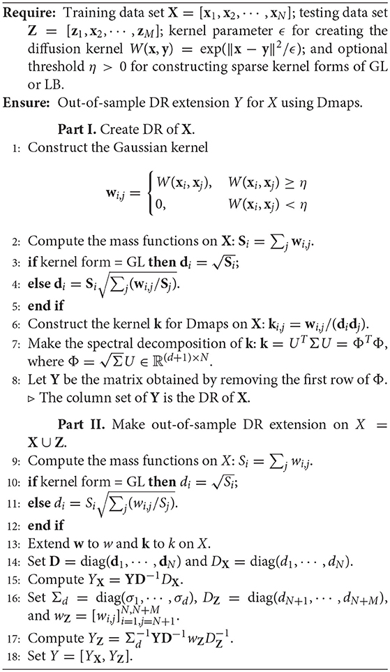
Algorithm 1: Out-of-Sample DR Extension for Dmaps

4. Illustrative Examples

In this section, we give several illustrative examples to show the validity of the Dmaps out-of-sample extensions. We employ four benchmark artificial data sets, S-curve, Swiss roll, punched sphere, and 3D cluster, in our samples. The graphs of these four data sets are give in Figure 1.

FIGURE 1

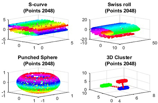
Figure 1. S-curve, Swiss Roll, Punched Sphere, and 3D-Cluster.

4.1. Out-of-Sample Extension by Graph-Laplacian Mapping

We first show the examples for the out-of-sample extensions provided by Graph-Laplacian mapping for the four benchmark figures. We set the size of each of these data sets by |X| = 2, 048. When the out-of-example algorithm is applied, we choose the size of the training data set to be |X| = 1, 843, which is 90% of the all samples, and choose the size of the testing set |Z| = 205, which is 10% of all samples. The parameters for the Graph-Laplacian kernel are set as follows: For obtaining the sparse kernel, we choose 25 nearest neighbors for every node, and assign the diffusion parameter ϵ = 1 for S-curve, Punched Sphere, and 3D Cluster, while assign ϵ = ∞ for Swiss Roll. We compare the DR result of the whole set X obtained by out-of-example extension with that obtained without out-of-example extension in the Figures 2–5. The figures show that the DRs obtained by out-of-sample extensions are satisfactory.

FIGURE 2

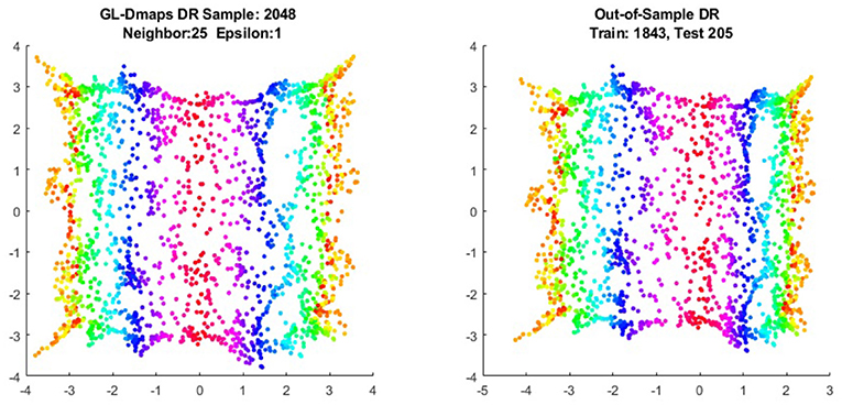
Figure 2. GL out-of-sample extension for DR of S-Curve.

FIGURE 3

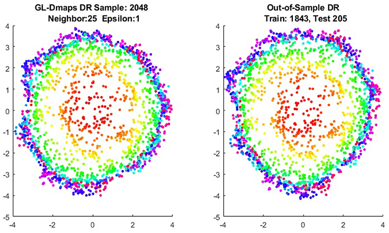
Figure 3. GL out-of-sample extension for DR of Punched Sphere.

FIGURE 4

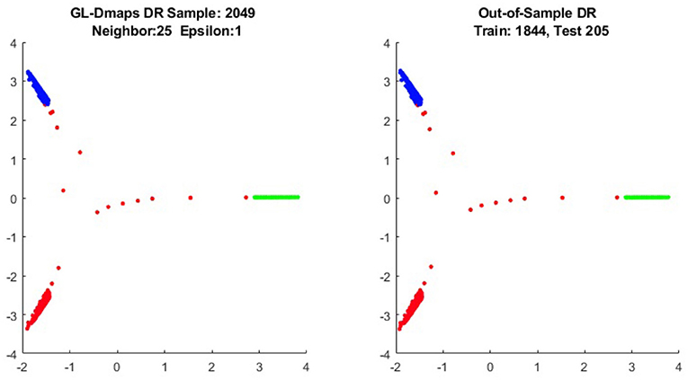
Figure 4. GL out-of-sample extension for DR of 3D Cluster.

FIGURE 5

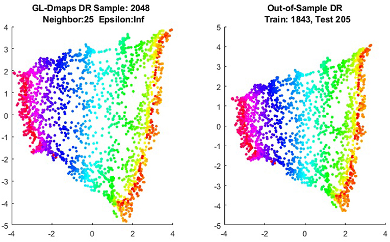
Figure 5. GL out-of-sample extension for DR of Swiss Roll.

4.2. Out-of-Sample Extension by Laplace-Beltrami Mapping

We now show the examples for the out-of-sample extensions provided by Laplace-Beltrami mapping for the same four benchmark figures. We set the same sizes for |X|,|X|, and |Z|, respectively. The parameters for the Laplace-Beltrami kernel are also set the same as for Graph-Laplacian kernel. The results of the comparisons are give in Figures 6–9.

FIGURE 6

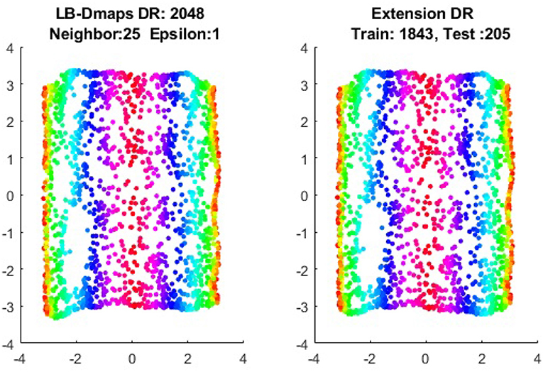
Figure 6. LB out-of-sample extension for DR of S-Curve.

FIGURE 7

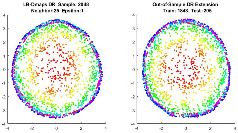
Figure 7. LB out-of-sample extension for DR of Punched Sphere.

FIGURE 8

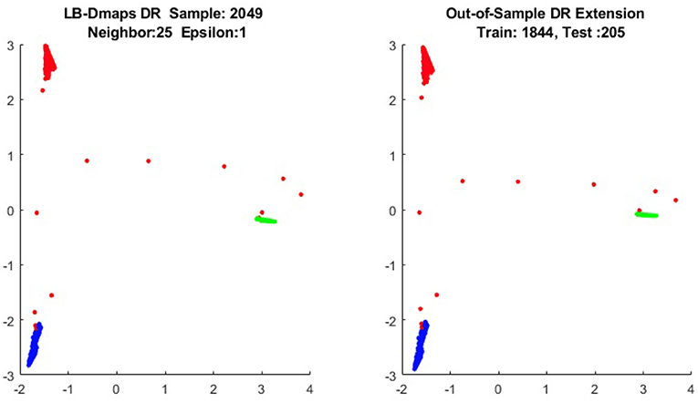
Figure 8. LB out-of-sample extension for DR of 3D Cluster.

FIGURE 9

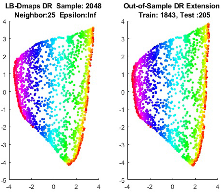
Figure 9. LB out-of-sample extension for DR of Swiss Roll.

To give more detailed comparisons, in Figures 10–13, we show the DRs of the training data and the testing data obtained by out-of-extensions and without extensions, respectively, for LB mapping.

FIGURE 10

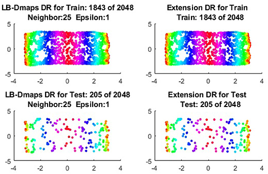
Figure 10. Comparisons of DRs of training data and the testing data, respectively, for S-curve.

FIGURE 11

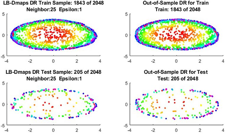
Figure 11. Comparisons of DRs of training data and the testing data, respectively, for Punched Sphere.

FIGURE 12

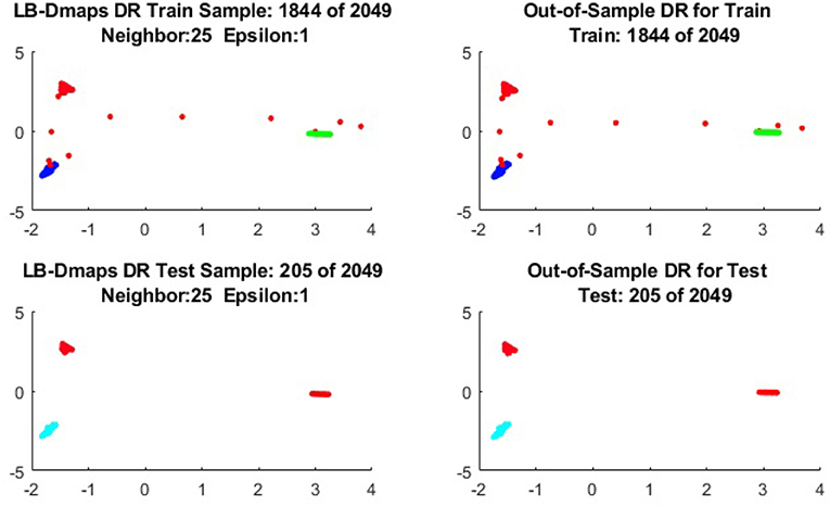
Figure 12. Comparisons of DRs of training data and the testing data, respectively, for 3D Cluster.

FIGURE 13

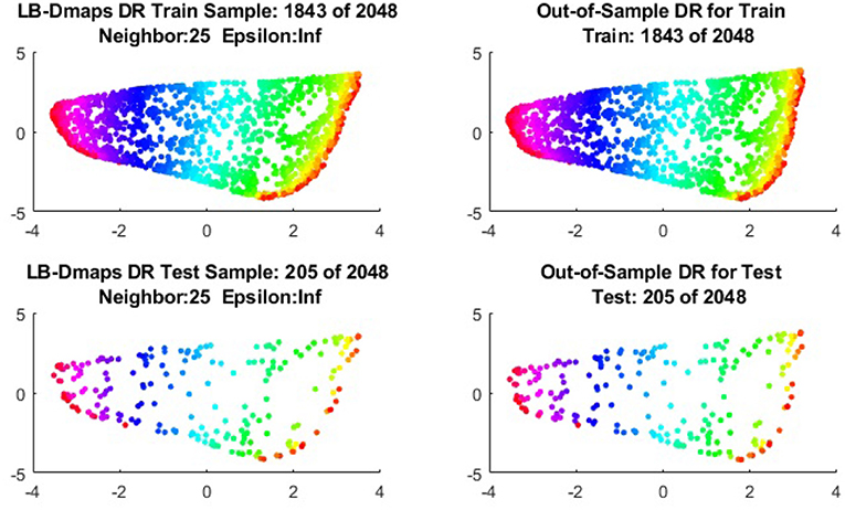
Figure 13. Comparisons of DRs of training data and the testing data, respectively, for Swiss Roll.

It is a common sense that if we reduce the size of the training set while increase the size for the testing set, the out-of-sample extension will introduce larger errors for DR. Figures 14–15 show that, in a relative large scope, say, the size of the testing set is no greater than the size of the training set. the out-of-sample extension still produces the acceptable results.

FIGURE 14

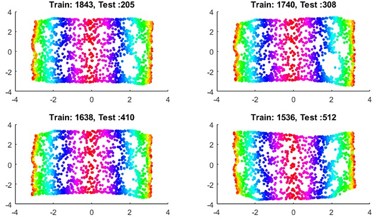
Figure 14. LB out-of-sample extension for different sizes of the test sets of S-curve (I).

FIGURE 15

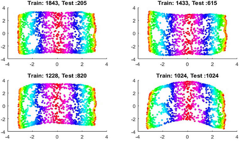
Figure 15. LB out-of-sample extension for different sizes of the test sets of S-curve (II).

Data Availability

No datasets were generated or analyzed for this study.

Author Contributions

The author confirms being the sole contributor of this work and has approved it for publication.

Conflict of Interest Statement

The author declares that the research was conducted in the absence of any commercial or financial relationships that could be construed as a potential conflict of interest.

References

1. Bellman R. Adaptive Control Processes: A Guided Tour. Princeton, NJ: Princeton University Press (1961).

Google Scholar

2. Scott DW, Thompson JR. Probability density estimation in higher dimensions. In: Gentle JE, editor. Computer Science and Statistics: Proceedings of the Fifteenth Symposium on the Interface. Amsterdam; New York, Ny; Oxford: North Holland-Elsevier Science Publishers (1983). p. 173–9.

Google Scholar

3. Lee JA, Verleysen M. Nonlinear Dimensionality Reduction. New York, NY: Springer (2007).

Google Scholar

4. Wang JZ. Geometric Structure of High-Dimensional Data and Dimensionality Reduction. Beijing; Berlin; Heidelberg: Higher Educaiton Press; Springer (2012).

Google Scholar

5. Jolliffe IT. Principal Component Analysis. Springer Series in Statistics. Berlin: Springer-Verlag (1986).

PubMed Abstract | Google Scholar

6. Zhang ZY, Zha HY. Principal manifolds and nonlinear dimensionality reduction via local tangent space alignment. SIAM J Sci Comput. (2004) 26:313–38.

Google Scholar

7. Schölkopf B, Smola A, Müller K-R. Nonlinear component analysis as a kernel eigenvalue problem. Neural Comput. (1998) 10:1299–319.

Google Scholar

8. Roweis ST, Saul LK. Nonlinear dimensionality reduction by locally linear embedding. Science. (2000) 290:2323–6. doi: 10.1126/science.290.5500.2323

PubMed Abstract | CrossRef Full Text | Google Scholar

9. Donoho DL, Grimes C. Hessian eigenmaps: new locally linear embedding techniques for high-dimensional data. Proc Natl Acad Sci USA. (2003) 100:5591–6. doi: 10.1073/pnas.1031596100

CrossRef Full Text | Google Scholar

10. Shmueli Y, Sipola T, Shabat G, Averbuch A. Using affinity perturbations to detect web traffic anomalies. In: The 11th International Conference on Sampling Theory and Applications (Bremen) (2013).

Google Scholar

11. Shmueli Y, Wolf G, Averbuch A. Updating kernel methods in spectral decomposition by affinity perturbations. Linear Algebra Appl. (2012) 437:1356–65. doi: 10.1016/j.laa.2012.04.035

CrossRef Full Text | Google Scholar

12. Balasubramanian M, Schwaartz E, Tenenbaum J, de Silva V, Langford J. The isomap algorithm and topological staility. Science (2002) 295:7. doi: 10.1126/science.295.5552.7a

PubMed Abstract | CrossRef Full Text | Google Scholar

13. Coifman RR, Lafon S. Diffusion maps. Appl Comput Harmon Anal. (2006) 21:5–30. doi: 10.1016/j.acha.2006.04.006

CrossRef Full Text | Google Scholar

14. Coifman RR, Lafon S. Geometric harmonics: a novel tool for multiscale out-of-sample extension of empirical functions. Appl Comput Harmon Anal. (2006) 2:31–52. doi: 10.1016/j.acha.2005.07.005

CrossRef Full Text | Google Scholar

15. Ng A, Jordan M, Weiss Y. On spectral clustering: analysis and an algorithm. Adv Neural Inform Process Syst. (2001) 14:849–56.

Google Scholar

16. Shi J, Malik J. Normalized cuts and image segmentation. IEEE Trans Pattern Anal Mach Intell. (2000) 22:888–905. doi: 10.1109/34.868688

CrossRef Full Text | Google Scholar

17. Belkin M, Niyogi P. Laplacian eigenmaps for dimensionality reduction and data representation. Neural Comput. (2003) 15:1373–96. doi: 10.1162/089976603321780317

CrossRef Full Text | Google Scholar

18. Aizenbud Y, Bermanis A, Averbuch A. PCA-based out-of-sample extension for dimensionality reduction. arXiv: 1511.00831 (2015).

Google Scholar

19. Bengio Y, Paiement J, Vincent P, Delalleau O, Le Roux N, Ouimet M. Out-of-sample extensions for LLE, Isomap, MDS, eigenmaps, and spectral clustering. In: Thrun S, Saul L, Schölkopf B, editors. Advances in Neural Information Processing Systems. Cambridge, MA: MIT Press (2004).

Google Scholar

20. Wang JZ. Mathematical analysis on out-of-sample extensions. Int J Wavelets Multiresol Inform Process. (2018) 16:1850042. doi: 10.1142/S021969131850042X

CrossRef Full Text | Google Scholar

21. Aronszajn N. Theory of reproducing kernels. Trans Amer Math Soc. (1950) 68:337–404.

Google Scholar