Modeling Variational Inpainting Methods With Splines

1. Introduction

In this paper we study the continuous inpainting problem for digital images. That is, our goal is to restore parts Ω of a digital image Ω′, Ω ⊂ Ω′ ⊂ ℝ^d, where the information has been removed, damaged, or is missing, from the remaining and well-maintained part. Naturally, this is only possible under suitable modeling assumptions on the image. For continuous images a common and practical model is that of a function of bounded variation as first studied in the well-known work of Rudin and Osher [1], and Rudin et al. [2]. For a numerical solution and its implementation, these models need to be discretized. For digital images, given by a set of pixels on a uniform grid, those functions and their derivatives are typically discretized using difference schemes for the pixel values. In this paper we rather use a finite dimensional function space, the space of tensor product spline functions based on B-splines, see e.g., [3, 4]. The advantage of this approach is that we avoid a pointwise discretization of the involved functions and derivatives. In addition, the compact support of the basis of B-splines contributes to an efficient and stable implementation.

In general, the inpainting problem involves recovering missing structure and missing texture. In this paper we focus on structural inpainting; for texture reconstruction other methods need to be used or added, see for example [5] and [6]. Also for structural inpainting there exists a variety of approaches. Examples include PDE-based methods (e.g., [5, 7–10]) and variational approaches as in [11–15]. Many of these methods can be combined with different models described by various finite dimensional function spaces [13, 15–18] which is also the approach we will follow in this paper. We especially want to point out the thesis of Hong [13] and the article of Hong et al. [15] which study a variational model similar to ours but using spline functions over triangulations. In our numerical section we also include some examples to compare the performance of our method with examples given in [13] and [15]. For a short survey of splines in image processing in general, see [19].

Naturally, this short summary cannot give a complete account of all related works. For example the problem of image completion (see [20] and references therein) is closely related. For a comprehensive overview to image processing from a mathematical perspective that also discusses inpainting, the authors recommend the books of Chan and Shen [21] as well as Aubert and Kornprobst [22].

Outline and Contribution

We will follow a variational approach by, roughly speaking, minimizing some functional over an extended inpainting area U(Ω) ⊃ Ω subject to constraints which ensure the reproduction of the well-maintained part of the image. Typically, the functional involves the image function u and some of its derivatives. The constraint, on the other hand, is chosen over some neighborhood B ⊆ Ω′ \ Ω of the inpainting area. We will model the class of functions for the variational method with tensor product B-splines together with a focus on total variation (TV) inpainting, [23], that is

$\begin{array}{ll}{\displaystyle {\int }_{U(\Omega )}}|\nabla u(x)|dx,& (1)\end{array}$

the effective, often used ROF-functional, see [2], which results in level curves of minimal length. Note that the application to this model is exemplary and the presented approach can be applied to other functionals as well.

We begin by giving some basic properties and notation for the tensor product splines used in this paper in section 2. Afterwards, in section 3 we show how to model the inpainting problem with those splines and analyze its properties. Numerical results are given in section 4. We present an algorithm and its implementation using a first-order primal-dual algorithm [24], compare the results of our method to standard TV inpainting and show some examples of applications.

2. Preliminaries and Notation

In the sequel, we will use the following notations and basic facts about B-splines and their derivatives. Even if images are usually considered in 2D, we will present the theory in an arbitrary number of variables; applications in higher dimensions would, for example include medical applications such as inpainting in voxel data provided by computerized tomography. The tensor product B-splines for inpainting which we will use in section 3 are defined over a rectangle $R={\otimes }_{j=1}^d\left[a_j,b_j\right]$, d ∈ ℕ. They are based on a tensor product knot grid which is given as

$\begin{array}{ll}T:={\otimes }_{j=1}^d\{{\tau }_{j,1},\dots ,{\tau }_{j,m_j+2n_j}\}& (2)\end{array}$

with τ_j,i < τ_j,i+nj for n_j ≤ i ≤ m_j + n_j. At the boundary, we request multiple knots

$\begin{array}{ll}\begin{array}{l}{\tau }_{j,1}=\cdots ={\tau }_{j,n_j}=a_j,\\ {\tau }_{j,m_j+n_j+1}=\cdots ={\tau }_{j,m_j+2n_j}=b_j,\end{array}& (3)\end{array}$

for n_j, m_j ∈ ℕ, 1 ≤ j ≤ d. We set n: = (n₁, …, n_d) and m: = (m₁, …, m_d) for the dimensions and degrees in the individual coordinates, respectively. The grid width h: = (h₁, …, h_d), defined as $h_j:={max}_k|{\tau }_{j,k}-{\tau }_{j,k+1}|$, is known to influence the approximation properties of the spline space. For $k\in \text{K}:={\otimes }_{j=1}^d\left\{1,\dots ,m_j+2n_j-1\right\}$ a grid cell is denoted by $Z_k:={\otimes }_{j=1}^d\left[{\tau }_{j,k_j},{\tau }_{j,k_j+1}\right]$.

The tensor product B-splines of order n with respect to the grid T are denoted by

$\begin{array}{ll}{B}_{\alpha }^n(x)={\displaystyle \prod _{j=1}^d}{B}_{{\alpha }_j}^{n_j}(x_j),\alpha \le m+n,& (4)\end{array}$

i.e., $\alpha \in {\text{I}}_{\text{m},n}:={\otimes }_{j=1}^d\left\{1,\dots ,m_j+n_j\right\}$. They have the support

$\begin{array}{ll}{S}_{\alpha }^n:={\otimes }_{j=1}^d{S}_{{\alpha }_j}^{n_j},S_{{\alpha }_j}^{n_j}:=[{\tau }_{j,{\alpha }_j},{\tau }_{j,{\alpha }_j+n_j}],& (5)\end{array}$

respectively. The spline space ${L}$ⁿ(T, Ω) of order n restricted to a domain Ω ⊂ ℝ^d is spanned by all B-splines $B_{\alpha }^n$ with $S_{\alpha }^n\cap \Omega \ne \varnothing$. The index set of all B-splines relevant for Ω is defined as ${\text{I}}_{\Omega }:=\{\alpha \in {\text{I}}_{m,n}|S_{\alpha }^n\cap \Omega \ne \varnothing \}$ and their number as #(I_Ω). If Ω = R, then I_R = I_{m, n} and $\#({\text{I}}_R)={\prod }_{j=1}^d{m}_j+n_j$.

A tensor product spline of order n with respect to T over a domain Ω is given by

$\begin{array}{ll}s(x)={\displaystyle \sum _{\alpha \in {\text{I}}_{\Omega }}}{g}_{\alpha }{B}_{\alpha }^n(x),x\in \Omega ,& (6)\end{array}$

with coefficients g_α ∈ ℝ. Let g = (g_α)_α∈IΩ and $\text{B}{(x)}^T:=(B_{\alpha }^n(x){)}_{\alpha \in {\text{I}}_{\Omega }}$ denote the vector of the coefficients and B-splines, respectively, then the spline s is given in matrix notation by s(x) = B(x)g.

With respect to inpainting methods an important property of the spline functions is that their derivatives can be expressed in terms of the coefficients of the spline function itself, that is

$\begin{array}{ll}{\partial }_{j}s(x):=\frac{\partial }{\partial x_j}s(x)={\displaystyle \sum _{\alpha \in {\text{I}}_{\Omega }}}{g}_{\alpha }{\partial }_j{B}_{\alpha }^n(x)& (7)\end{array}$

where

$\begin{array}{ll}{\partial }_j{B}_{\alpha }^n(x):=\frac{\partial }{\partial x_j}{B}_{\alpha }^n(x)=(n_j-1)\left(\frac{B_{\alpha }^{n-{\epsilon }_j}(x)}{|S_{{\alpha }_j}^{n_j-1}|}-\frac{B_{\alpha +{\epsilon }_j}^{n-{\epsilon }_j}(x)}{|S_{{\alpha }_j+1}^{n_j-1}|}\right)& (8)\end{array}$

denotes the derivative of the B-splines. Here, ε_j is the j-th unit vector.

The ℓ^p-norm of vectors will be denoted by ‖·‖_p and the L^p-norm of functions by ‖·‖_{p, Ω}.

3. Modeling of Inpainting Problem

Assume we want to reproduce a rectangular image Ω′ ⊂ ℝ^d by a tensor product spline. This can easily be done by choosing a tensor product grid with multiple knots on the boundary ∂Ω′ such that Ω′ is the domain of definition. This method guarantees that the B-spline basis is stable.

Theorem 1. For any rectangular domain $R={\otimes }_{j=1}^d\left[a_j,b_j\right]$, d ∈ ℕ, and any spline order $n=(n_1,\dots ,n_d)\in {\mathbb{N}}^d$, the B-spline basis ${\{B_{\alpha }^n(x)\}}_{\alpha \in {\text{I}}_{m,n}}$ with respect to knots defined as in (2) and (3) is stable, that is, there exist constants c, C > 0 such that

$\begin{array}{ll}c{\Vert g\Vert }_p\le {\Vert Bg\Vert }_{p,\Omega }\le C{\Vert g\Vert }_p,g\in {ℝ}^{I_{\Omega }},& (9)\end{array}$

The constants are only depending on n and d.

Due to the tensor product structure and the multiple knots on the boundary, this result can be proven analogously to the classical univariate results for intervals, see, e.g., [25]. For further information about stability of tensor product B-spline bases see for example [26]. In addition to stability, multiple knots on the boundary of R help us to avoid artifacts at the boundary since they result in an interpolation at the boundary and, thus, satisfying a non-homogeneous Dirichlet boundary condition.

We introduce a general version of our interpolation problem before stating the concrete model for which we give proofs and examples. It seems worthwhile, however, to mention that it also works with other models. For arbitrary Ω′ ⊂ ℝ^d, the inpainting problem considered here can be described in the following way: Given two bounded domains Ω and Ω′ such that

1. Ω ⊂ Ω′ ⊂ ℝ^d,

2. there exists $R={\otimes }_{j=1}^d\left[a_j,b_j\right]$ such that Ω ⊂ R ⊆ Ω′ and ∂Ω ∩ ∂R = ∅.

The goal is to reconstruct a function or picture f on Ω that is known only on Ω^*: = Ω′ \ Ω by using tensor product splines defined over R. The situation is illustrated in Figure 1. Note that in case of multiple disconnected unknown inpainting areas, as for example illustrated in the left image of Figure 3, the method can be applied for each area separately. For easier comparability we choose R = Ω′ for all of our examples considered in section 4.

FIGURE 1

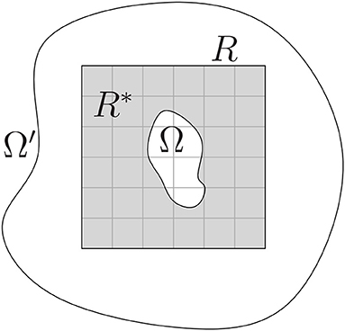
Figure 1. Illustration of domains.

We require that the spline fulfills a side condition on R^*: = R \ Ω ⊂ Ω^* and minimizes a functional F over some neighborhood U(Ω) including Ω. The general variational inpainting model using splines can now be formulated as follows.

Spline Inpainting Model 1. Let $U_h^n(\Omega )$ be some neighborhood of Ω only depending on h and n with $\Omega \subseteq U_h^n(\Omega )\subseteq R$. The spline inpainting model is given by: Determine s∈ ${L}$ⁿ(T, R) by

$\begin{array}{llll}minimize& F(s,\nabla s,\dots )(x)& forx\in U_h^n(\Omega )& (10)\end{array}$

$\begin{array}{llll}subjectto& s(x)=f(x)& forx\in R^{*}.& (11)\end{array}$

Remark 1. Since hard constraints can be problematic, especially in the presence of noise, the minimization problem is often relaxed to

$\begin{array}{ll}minimizeF\left(s,\nabla s,\dots \right){|}_{U_h^n(\Omega )}+\frac{\epsilon }{2}\Vert s-f{\Vert }_{2,R^{*}}^2& (12)\end{array}$

for some ε > 0. This relaxed formulation will be discussed briefly in section 4.

For the explicit modeling or the discretization of the Spline Inpainting model 1, the concrete functional in the minimization is, of course, crucial. As already mentioned in section 1, we will follow one of the first important approaches and focus on TV inpainting [23] and, therefore, on the ROF-functional [2].

Spline Inpainting Model 2. Let $U_h^n(\Omega )$ be some neighborhood of Ω only depending on h and n with $\Omega \subseteq U_h^n(\Omega )\subseteq R$. The TV spline inpainting model is given by: Determine s ∈ ${L}$ⁿ(T, R) by

$\begin{array}{lll}minimize& {\int }_{U_h^n(\Omega )}|\nabla s(x)|dx& (13)\end{array}$

$\begin{array}{llll}subjectto& s(x)=f(x)& forx\in R^{*},& (14)\end{array}$

where $|\nabla s(x)|:=\sqrt{\sum _{i=1}^d({\partial }_{i}s(x){)}^2}$.

Considering discrete problems (e.g., digital images) and, thus, a discrete set of points, the constraint coincides with an interpolation of a finite set of points. To apply the interpolation, usually, a discretization of all involved functions and derivatives is necessary. In the next two subsections we show that for the continuous Spline Inpainting Models 2 only the discretization of the integral over grid cells Z_k in a neighborhood of the inpainting area Ω is needed. Note that Theorem 2 concerning the constraint also holds true in case of the general model Spline Inpainting Model 1. Theorem 3 treats the special functional considered in (13). Nevertheless, the decomposition in (32) as well as the representation of the involved spline functions and derivatives remain the same. Thus, depending on concrete given functional Theorem 3 and the Discrete Spline Inpainting Model 1 would have to be adapted. As a simple approach one could use the squared gradient norm in (13), i.e., |∇s(x)|². This puts a stronger penalty term on large gradients what can be useful for large inpainting areas. We will also test this approach in the numerical section of this work. In case of the often considered Laplace and biharmonic equations (e.g., [17] and references therein) our spline approach would reduce to a linear system with respect to the coefficients of the spline function.

Clearly, there are different possible interpretations of a discrete image. In our situation, where we evaluate functions at points in R, those interpretations influence the value of the image that we assume to be at that points. Since it does not change the method or modeling, we interpret, for the sake of simplicity, the discrete values as piecewise constant functions with constant values over rectangles. This means, for an image f considered over $R={\otimes }_{j=1}^d[a_j,b_j]$ consisting of μ₁× ⋯ × μ_d pixels, the single pixels are defined as uniform rectangles $P_{\beta }:={\otimes }_{j=1}^d[a_j+({\beta }_j-1)p_j,a_j+{\beta }_j{p}_j)$ for p_j: = (b_j − a_j)/μ_j and 1 ≤ β_j ≤ μ_j. The value of the image over P_β is chosen corresponding to the value at the center $c(P_{\beta }):=\text{(}{a}_j+({\beta }_j-\frac{1}{2})p_j{\text{)}}_{j=1}^d$ of this pixel; the j-th coordinate will be denoted by c(P_β)j.

3.1. Constraint

In the reproduction of digital images on R^*, the constraint (14) corresponds to the interpolation of the pixel values in R^*. We use the centers of the pixels c(P_β) as those interpolation points. In the space of tensor product splines an interpolation problem is solvable if the number of interpolation points is not greater than the degrees of freedom #(I_R) and if there is a relationship between the interpolation sites and the knots, known as the Schoenberg–Whitney condition. Since we also need some degrees of freedom for the minimization problem over U(Ω), this forces us to choose a spline space of sufficiently large dimension.

Definition 1. Given a tensor product grid T over R and a set of discrete points $\Xi :=\{{\xi }_{\beta }\in R|\beta \in {\mathbb{Z}}^d;\#(\beta )\le \#({\text{I}}_R)\}$, let λ_β be the point evaluation functionals λ_β(g): = g(ξ_β), g : Ξ → ℝ. A spline s ∈ ${L}$ⁿ(T, R) is the spline interpolant of a function g at Ξ if

$\begin{array}{ll}{\lambda }_{\beta }(s)={\displaystyle \sum _{\alpha \in {\text{I}}_R}}{g}_{\alpha }{B}_{\alpha }^n({\xi }_{\beta })={\lambda }_{\beta }(g),{\xi }_{\beta }\in \Xi .& (15)\end{array}$

For functions defined over R and grids T satisfying (2) and (3) this interpolation problem is uniquely solvable if the Schoenberg-Whitney condition (see, e.g., [27]) is satisfied. Since R is a rectangle, this can be guaranteed by choosing the tensor product Greville abscissae as interpolation sites, that is, by setting

$\begin{array}{ll}{\Xi }_{Gr}:=\{{\xi }_{\gamma }\in {ℝ}^d\text{|}{\xi }_{\gamma }{,}_j:=\frac{1}{n_j-1}{\displaystyle \underset{i=1}{\overset{n_j-1}{{\sum }^{\text{}}}}}{\tau }_{j,{\gamma }_j+i},\gamma \in {\text{I}}_R\}.& (16)\end{array}$

It should be noted that the position of the Greville abscissae depends on the position of the knots of T, hence, the interpolation points depend on T. Since the centers of the pixels in R^* need to be interpolated, we have to choose a knot grid such that those are contained in the set of Greville abscissae. In case of digital images, where each rectangle P_β represents a pixel of the image, we have the following result for the reproduction of all known image pixel values.

Theorem 2. Given an image f of size ${\otimes }_{j=1}^d{\mu }_j$, an area $R^{*}:={\cup }_{\beta \in {\text{J}}_{R^{*}}}{P}_{\beta }$, ${\text{J}}_{R^{*}}:=\left\{\beta \in {\mathbb{Z}}^d:1\le {\beta }_j\le {\mu }_j,1\le j\le d\mathrm{\text{ and }}c(P_{\beta })\in R\backslash \Omega \right\}$ of known pixel values and an order n of a spline space, there exist a knot grid T and a set of interpolation points Ξ^* such that

$\begin{array}{ll}{\{c(P_{\beta })\}}_{\beta \in {\text{J}}_{R^{*}}}\subset {\Xi }^{*},{\lambda }_{\gamma }(s)={\lambda }_{\gamma }(f),{\xi }_{\gamma }\in {\Xi }^{*},& (17)\end{array}$

for s∈ ${L}$ⁿ(T, R).

Proof: Due to the tensor product structure, it suffices to consider a single coordinate direction j for the construction of the grid and set of interpolation points.

In doing so, we have to distinguish between even and odd values of n_j. We set m_j = μ_j − 1 for n_j odd and m_j = μ_j otherwise, and choose

$\begin{array}{ll}\{\begin{array}{ll}{\tau }_{j,n_j+k_j}:=a_j+k_j·p_j& n_j\text{\hspace{0.17em}odd},\\ {\tau }_{j,n_j+k_j}:=a_j+(k_j-\frac{1}{2})·p_j& n_j\text{\hspace{0.17em}even}\end{array}& (18)\end{array}$

for 1 ≤ k_j ≤ m_j and $p_j:=\frac{b_j-a_j}{{\mu }_j}$. The boundary knots are determined with proper multiplicity according to (3). Recalling (16), the j-th coordinates of the associated Greville abscissae for odd n_j are given by

$\begin{array}{ll}{\xi }_{\gamma },j=\{\begin{array}{ll}{a}_j\hfill & \text{for }{\gamma }_j=1,\hfill \\ a_j+\frac{p_j}{n_j-1}\left({\displaystyle \underset{\ell =1}{\overset{{\gamma }_j-1}{\sum ^{\text{}}}}}\ell \right)\hfill & \text{for }\begin{array}{l}{\gamma }_j\ge 2\\ {\gamma }_j\le n_j-1,\end{array}\hfill \\ a_j+\frac{p_j}{n_j-1}\left({\displaystyle \underset{\ell ={\gamma }_j+1-n_j}{\overset{{\gamma }_j-1}{\sum ^{\text{}}}}}\ell \right)\hfill & \text{for }\begin{array}{l}{\gamma }_j\ge n_j\\ {\gamma }_j\le m_j+1,\end{array}\hfill \\ b_j-\frac{p_j}{n_j-1}\left({\displaystyle \underset{\ell =1}{\overset{m_j+n_j-{\gamma }_j}{\sum ^{\text{}}}}}\ell \right)\hfill & \text{for }\begin{array}{l}{\gamma }_j\ge m_j+2\\ {\gamma }_j\le m_j+n_j-1,\end{array}\hfill \\ b_j\hfill & \text{for }{\gamma }_j=m_j+n_j.\hfill \end{array}& (19)\end{array}$

Replacing the terms ℓ of the sums by ℓ − 1/2, results in the Greville abscissae for even n_j, respectively. Therefore, we have

$\begin{array}{ll}{\xi }_{\gamma },j=\{\begin{array}{ll}{a}_j+\frac{({\gamma }_j-1){\gamma }_j}{2(n_j-1)}{p}_j& \text{for }\begin{array}{l}{\gamma }_j\ge 1\\ {\gamma }_j\le n_j-1,\end{array}\\ a_j+({\gamma }_j-\frac{n_j}{2})p_j& \text{for }\begin{array}{l}{\gamma }_j\ge n_j\\ {\gamma }_j\le m_j+1,\end{array}\\ b_j-\frac{(m_j+n_j-{\gamma }_j+1)(m_j+n_j-{\gamma }_j)}{2(n_j-1)}{p}_j& \text{for }\begin{array}{l}{\gamma }_j\ge m_j+2\\ {\gamma }_j\le m_j+n_j.\end{array}\end{array}& (20)\end{array}$

for odd n_j and

$\begin{array}{ll}{\xi }_{\gamma },j=\{\begin{array}{ll}{a}_j& \text{for }{\gamma }_j=1,\\ a_j+\frac{{({\gamma }_j-1)}^2}{2(n_j-1)}{p}_j& \text{for }\begin{array}{l}{\gamma }_j\ge 2\\ {\gamma }_j\le n_j-1,\end{array}\\ a_j+({\gamma }_j-\frac{n_j+1}{2})p_j& \text{for }\begin{array}{l}{\gamma }_j\ge n_j\\ {\gamma }_j\le m_j+1,\end{array}\\ b_j-\frac{{(m_j+n_j-{\gamma }_j)}^2}{2(n_j-1)}{p}_j& \text{for }\begin{array}{l}{\gamma }_j\ge m_j+2\\ {\gamma }_j\le m_j+n_j-1,\end{array}\\ b_j& \text{for }{\gamma }_j=m_j+n_j.\end{array}& (21)\end{array}$

for even n_j, respectively. Now ξ_{γ, j} coincides, for n_j ≤ γ_j ≤ m_j + 1, with c(P_β)_j for some 1 ≤ β_j ≤ μ_j; more precisely, with centers c(P_β)_j such that

$\begin{array}{ll}{\beta }_j\in \stackrel{\circ }{\text{I}}:=\{\begin{array}{cc}\{\frac{n_j+1}{2},\dots ,{\mu }_j-\frac{n_j-1}{2}\}& \text{for odd\hspace{0.17em}}{n}_j\\ \{\frac{n_j}{2},\dots ,{\mu }_j+1-\frac{n_j}{2}\}& \text{for even\hspace{0.17em}}{n}_j\end{array}.& (22)\end{array}$

The Greville abscissae of boundary B-splines, that is, of B-splines with some knots at a_j or b_j, are not necessarily placed at a center, but they can be replaced by the center that is closest to them without loss of the Schoenberg-Whitney condition $B_{{\gamma }_j}^{n_j}({\xi }_j)>0$, due to property (5).

We now claim: For every ${\beta }_j\in \left\{1,\dots ,{\mu }_j\right\}\backslash \stackrel{\bullet }{\text{I}}$, there exists γ_j such that

$\begin{array}{ll}-\frac{1}{2}{p}_j<{\xi }_{\gamma ,j}-c{(P_{\beta })}_j\le \frac{1}{2}{p}_j.& (23)\end{array}$

There are four cases to be considered: small and large β_j (or γ_j) and even or odd order. We prove the claim for small β_j or γ_j and odd order, the other cases can be verified in the same way. For γ_j ∈ {2, …, n_j − 1} and odd n_j we have

$\begin{array}{ll}{\xi }_{\gamma }{,}_j-c{(P_{\beta })}_j=\left(\frac{({\gamma }_j-1){\gamma }_j}{2(n_j-1)}-{\beta }_j+\frac{1}{2}\right)·p_j.& (24)\end{array}$

Therefore, we need to show that for every β_j ∈ {1, …, (n_j − 1)/2} there exists a γ_j ∈ {2, …, n_j − 1} such that

$\begin{array}{ll}{\beta }_j-1<\frac{({\gamma }_j-1){\gamma }_j}{2(n_j-1)}\le {\beta }_j.& (25)\end{array}$

Set $h({\gamma }_j):=\frac{({\gamma }_j-1){\gamma }_j}{2(n_j-1)}$. Then we have 0 < h(2) ≤ 1 and $\frac{n_j-1}{2}-1<h(n_j-1)\le \frac{n_j-1}{2}$. As a consequence, $0<h({\gamma }_j)\le \frac{n_j-1}{2}$ for all γ_j ∈ {2, …, n_j − 1}. Clearly, h(γ_j) is monotonically increasing and #γ_j = n_j − 2 distributed over (n_j − 1)/2 intervals. Further, $h({\gamma }_j)-h({\gamma }_j-1)=\frac{{\gamma }_j-1}{n_j-1}\le 1$ and, thus, the claim is valid.

Having this property at hand, we replace those ξ_{γ, j} by c(P_β)_j that are closest to the center, to guarantee that all centers are contained in the set of interpolation points. For $\beta \in \{1,\dots ,{\mu }_j\}\backslash \stackrel{\bullet }{\text{I}}$ set

$\begin{array}{ll}\begin{array}{l}\tilde{\text{I}}:=\{{\gamma }_j\in \text{{}1,\dots ,m_j+n_j\text{}}:{\xi }_{\gamma ,j}=\underset{{}_{{\tilde{\gamma }}_j}}{\min }\text{{}{\text{argmin}}_{{\xi }_{\tilde{\gamma },j}}\text{|}{\xi }_{{}_{\tilde{\gamma },j}}-c{(P_{\beta })}_j|\}\}\hfill \end{array}& (26)\end{array}$

and

$\begin{array}{ll}{\tilde{\xi }}_{\gamma ,j}:={\text{argmin}}_{c{(P_{\beta })}_j}|{\xi }_{\tilde{\gamma },j}-c{(P_{\beta })}_j|\text{for }{\gamma }_j\in \tilde{\text{I}}.& (27)\end{array}$

The set

$\begin{array}{ll}{\Xi }_j:=\left\{{\xi }_{\gamma ,j}:{\gamma }_j\in \{1,\dots ,m_j+n_j\}\backslash \tilde{\text{I}}\right\}\cup \left\{{\tilde{\xi }}_{\gamma ,j}:{\gamma }_j\in \tilde{\text{I}}\right\}& (28)\end{array}$

gives us the j-th coordinate of Ξ, the set of possible interpolation points. Finally, the set Ξ^* of interpolation points is determined by restriction of Ξ to R^*, that is ${\xi }_{\gamma }\in {\Xi }^{*}:=\Xi \cap R^{*}$. By construction, $c(P_{\beta })\in {\Xi }^{*}$ for $\beta \in {\text{J}}_{R^{*}}$ and there exists a spline interpolant s ∈ ${L}$ⁿ(T, R) for f at Ξ^*.□

In the sequel, Ξ and Ξ^* always will refer to the sets of interpolation sites determined in the way described in the proof of Theorem 2. For applications we also want to describe the constraints in matrix notation. For the coefficients $\text{g}=(g_{\alpha }{)}_{\alpha \in {\text{I}}_R}\in {ℝ}^{\#({\text{I}}_R)}$, we get

$\begin{array}{ll}{\text{s}}_{{\Xi }^{*}}={\text{B}}_{{\Xi }^{*}}\text{g}={\text{f}}_{{\Xi }^{*}}& (29)\end{array}$

with

$\begin{array}{ll}{f}_{{\Xi }^{*}}={\left(f({\xi }_{\beta })\right)}_{\beta \in {\Xi }^{*}}\in {ℝ}^{\#({\Xi }^{*})},& (30)\end{array}$

$\begin{array}{ll}{B}_{{\Xi }^{*}}=\left[B_{\alpha }^n({\xi }_{\beta }):{}_{\alpha \in {\text{I}}_R}^{{\xi }_{\beta }\in {\Xi }^{*}}\right]\in {ℝ}^{\#({\Xi }^{*})\times \#({\text{I}}_R)}.& (31)\end{array}$

3.2. Minimization

Depending on Ω, there are still some degrees of freedom left for minimization; their number is given by #(Ξ \ Ξ^*). We define $U_T^n(\Omega )$ as the union of all supports of B-splines corresponding to ${\xi }_{\alpha }\in \Xi \backslash {\Xi }^{*}$, that is

$\begin{array}{ll}{U}_T^n(\Omega ):={\displaystyle \bigcup _{\alpha \in {\text{I}}_R\backslash {\text{I}}_{{\Xi }^{*}}}}{S}_{\alpha }^n.& (32)\end{array}$

The index set of all cells in $U_T^n(\Omega )$ is denoted by ${\text{K}}_{\Omega }:=\{k\in \text{K}|Z_k\subset U_T^n(\Omega )\}$.

Proposition 3. Given T and Ω ⊂ R. For $U_T^n(\Omega )$ defined as in (32), the minimization problem (13) reduces to

$\begin{array}{ll}{\displaystyle \underset{\text{g}}{min}}{\displaystyle \sum _{k\in {\text{K}}_{\Omega }}}{\displaystyle {\int }_{Z_k}}|({\text{B}}^j(x)g{)}_{j=1}^d|dx,& (33)\end{array}$

where g = (gα)_{α ∈ IΩ}, gα ∈ ℝ, and

$\begin{array}{ll}\begin{array}{l}{[B^j(x)]}^T:={({\partial }_j{B}_{\alpha }^n(x))}_{\alpha \in {\text{ I}}_R}\in {ℝ}^{\#({\text{I}}_R)}.\hfill \end{array}& (34)\end{array}$

Remark 2. It is worthwhile to point out that the derivatives ${\partial }_j{B}_{\alpha }^n(x)$ are just weighted differences of B-splines of lower order, the explicit formula being given in section 2. This fact is of crucial importance for the efficient implementation of the method as it leads to sparse difference matrices.

Proof of Proposition 3: The result follows by applying (7) and (32). The first one directly gives us $\nabla s(x)=({\text{B}}^j(x)\text{g}{)}_{j=1}^d$ with unknown coefficients g. The area of integration $U_T^n(\Omega )$ consists of a union of grid cells and, thus, the integral can be split up into those grid cells Z_k for k ∈ K_Ω.□

Typically, for digital images the integration and the derivatives need to be discretized, as already mentioned in section 1. In our case, we only need to discretize the integral and the way the problem is modeled helps with that, too: the discretization of the integrals can be done simply and efficiently by using a Gaussian quadrature formula for the grid cells Z_k for k ∈ K_Ω. The tensor product structure allows us to use the univariate Gauss-Legendre quadrature formula in each coordinate direction. Let $\Theta \subset U_T^n(\Omega )$ be the set of the nodes of the Gauss-Legendre quadrature and w_θ be the corresponding weights. We get

$\begin{array}{ll}{\displaystyle \sum _{k\in {\text{K}}_{\Omega }}}{\displaystyle {\int }_{Z_k}}|({\text{B}}^j(x)\text{g}{)}_{j=1}^d|dx\approx {\displaystyle \sum _{\theta }}{w}_{\theta }\Vert ({\text{B}}^j(\theta )\text{g}{)}_{j=1}^d{\Vert }_2,& (35)\end{array}$

where ‖·‖₂ denotes the Euclidean norm.

Discrete Spline Inpainting Model 1. Using Proposition 3 and 2 [or (29)] the discrete form of TV Spline Inpainting Model 2 is given by: Determine s ∈ ${L}$ⁿ(T, R) by

$\begin{array}{ll}{minimize}_{g_{\alpha }}& {\displaystyle {\sum }_{\theta \in \Theta }}{w}_{\theta }\Vert {\text{B}}_{\theta }\text{g}\Vert {}_2\\ \text{ subject to}& {\text{ B}}_{{\Xi }^{*}}\text{g}={\text{f}}_{{\Xi }^{*}}\end{array}$

where ${\text{B}}_{\theta }:=({\text{B}}^j(\theta ){)}_{j=1}^d\in {ℝ}^{d\times \#({\text{I}}_R)}$.

This approach is also suitable for other types of Spline Inpainting Models 1, as long as the functionals depend on the function and its derivatives and it can be applied as soon as the explicit functional is given.

4. Numerical Implementation and Experiments

Define the convex operators F : ℝ^{d× #(Θ)} → ℝ and $G:{ℝ}^{\#({\text{I}}_{\Omega })}\to ℝ$ with

$\begin{array}{ll}\begin{array}{c}F(x_1,\dots ,x_{\#(\Theta )})={\displaystyle \underset{k=1}{\overset{\#(\Theta )}{{\sum }^{\text{}}}}}{\Vert x_k\Vert }_2,\end{array}& (36)\end{array}$

$\begin{array}{ll}G(g)=\{\begin{array}{ll}0\hfill & B_{{\Xi }^{\ast }}g=f_{{\Xi }^{\ast }},\hfill \\ \infty \hfill & \text{otherwise},\hfill \end{array}& (37)\end{array}$

and the linear operator $K:{ℝ}^{\#({\text{I}}_{\Omega })}\to {ℝ}^{2\times \#(\Theta )}$ with K(g) = (_{wθBθg)θ ∈ Θ}. Using this, the Discrete Spline Inpainting Model 1 can be reformulated as an optimization problem in the following way:

Optimization Problem 1. Our Spline Inpainting Model 1 is equivalent to the unconstrained problem

$\begin{array}{lll}minimize& & F(K\text{g})+G(\text{g}).\end{array}$

This formulation is suitable for the first-order primal-dual algorithm presented in [24]. Therefore, the λ-proximity operators ${prox}_{\lambda F^{*}}$, prox_λG need to be calculated. Note that the convex conjugate function F^*:ℝ^{d× #(Θ)} → ℝ is given by

$\begin{array}{ll}{F}^{*}(y_1,\dots ,y_{\#(\Theta )})=\{\begin{array}{ll}0& {\Vert y_k\Vert }_2\le 1, \forall k\le \#(\Theta )\\ \infty & \text{otherwise}\end{array}.& (38)\end{array}$

Both, F^* and G are indicator functions and, thus, the proximity operators are equivalent to the projections:

$\begin{array}{ll}\begin{array}{c}\underset{\lambda F^{*}}{prox}(y_1,\dots ,y_{\#(\Theta )})=\left(\frac{y_1}{\max (1,\Vert y_1{\Vert }_2)},\dots ,\frac{y_{\#(\Theta )}}{\max (1,\Vert y_{\#\Theta }{\Vert }_2)}\right),\end{array}& (39)\end{array}$

$\begin{array}{ll}\underset{\lambda G}{prox}(g)=g-B_{{\Xi }^{*}}^{+}(B_{{\Xi }^{*}g}-f_{{\Xi }^{*}}),& (40)\end{array}$

where ${\text{B}}_{{\Xi }^{*}}^{+}$ is the pseudoinverse of the rectangular matrix ${\text{B}}_{{\Xi }^{*}}$. We remark that both operators are independent of λ. In our experiments, we use the MATLAB implementation of the primal-dual solver due to Gabriel Peyre [28] and apply the tests to several cartoon-like images and natural images in different sizes; some are shown in Figure 2.

FIGURE 2

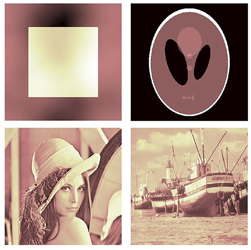
Figure 2. Exemplary test data: cartoon-like images and natural images.

We consider two different scenarios for the inpainting region Ω. In one scenario, the image is damaged by one or several “scratches” of variable width; in the second case we consider randomly missing pixels similar to “salt-and-pepper” noise. Figure 3 gives an example for both types (in comparison to Figure 2 the contrast is changed to emphasize the inpainting area).

FIGURE 3

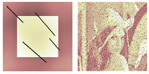
Figure 3. Considered inpainting area types: Scratches (Left) and randomly missing pixels (Right).

In the next subsection we discuss the optimal spline order for the inpainting problem as well as reasonable strategies to guess a starting value for the primal-dual algorithm. We compare our results with the standard TV inpainting using, again, an implementation by Gabriel Peyre [28]. Afterwards, we demonstrate the benefits of our method by two examples: Text removal and salt-and-pepper denoising.

4.1. Numerical Evaluation

4.1.1. Starting Guess

Both implementations, spline inpainting and standard TV inpainting, are iterative methods. Thus, they rely on a suitable initial value to return a good solution after a reasonable number of iterations. We tried several strategies among which two stood out and will be detailed in what follows. In a first strategy we choose random uniformly distributed values in [0, 255] (for standard grayscale images). Note that standard TV inpainting directly iterates on the pixel values of the inpainting area while our spline approach works on the spline coefficients as its variables. Thus, although both algorithms use uniformly distributed values, the starting guess strategies differ slightly. For our second strategy, we calculate the mean value ω_mean of the image outside the inpainting area. In contrast to that, standard TV sets the pixels inside the inpainting area to ω_mean. Our spline approach uses the starting values g = prox_λG(ω_mean1), where 1 is a vector of ones. Since splines form a partition of unity, the coefficient vector ω_mean1 generates a constant image with value ω_mean. Using prox_λG, this vector is projected onto the interpolation space.

Figure 4 illustrates the peak signal-to-noise ratio (PSNR) for both starting strategies using 300 experiments on several images (128 × 128 pixels) and inpainting areas after 100 iterations. We use two types of inpainting areas: on the one hand 3% of the pixels are randomly set to zero (left), on the other hand 3 scratches with a 4 pixel width are used (right). The mean PSNR is calculated for cartoon-like images (top) and natural images (bottom) separately.

FIGURE 4

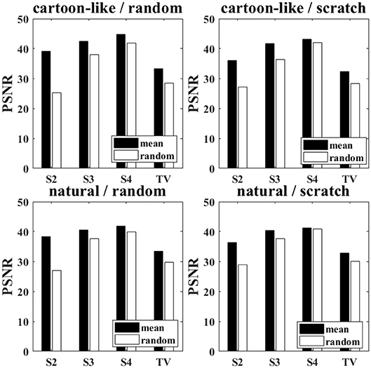
Figure 4. Obtained PSNR values using random starting guess (white) or mean value (black). (Left): random inpainting area (3% of the pixels); (Right): scratches (3 scratches, 4 pixels width); top: cartoon-like images; bottom: natural images.

We see that the mean value starting guess performs better for all combinations of image and noise type. However, the effect seems to be stronger for a small spline order. Also, random missing pixel noise is more influenced by the starting guess strategy than scratch inpainting. In Figure 5 a visual comparison of both reconstructions is given. The “Lena” image shown in Figure 3 with randomly missing pixels is inpainted with splines of order 2; first with random starting guess and a second time with mean value. The obtained PSNR values are 26.21 and 31.80, respectively.

FIGURE 5

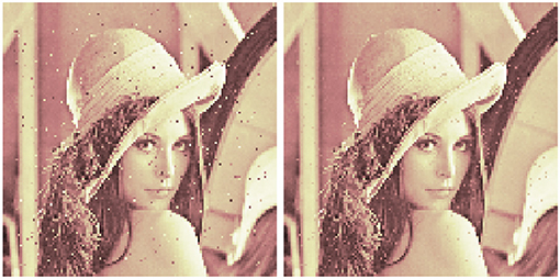
Figure 5. Reconstruction of Lena (see Figure 3) using splines of order 2 with random starting guess (left) and mean value strategy (right).

4.1.2. Spline Order

Figure 4 already makes clear that a higher spline order yields a better reconstruction. We analyze this in more details in the next experiment. Again, we calculate the mean PSNR over 300 runs using 128 × 128 pixel images. This time, we plot the PSNR against the percentage of unknown pixels (random inpainting area) or scratch width (scratch inpainting area) for both image types. Figure 6 shows the obtained PSNR for different spline orders and standard TV as comparison. For both algorithms, we use the optimal starting guess just discussed.

FIGURE 6

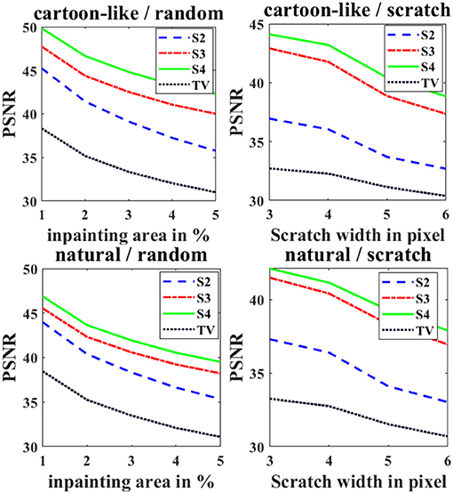
Figure 6. Obtained PSNR values for different spline orders and standard TV. Left: random inpainting area; right: scratches; top: cartoon-like images; bottom: natural images.

We can clearly see that a higher spline order in all cases performs a better reconstruction. However, the difference is not as strong for small inpainting areas, such as the randomly missing pixels. Moreover, the effect dimishes when going from order 3 to 4 which yield nearly similar results. Note that all spline orders clearly outperform standard TV inpainting. Thus, we recommend to use at least splines of order 3.

Figure 7 gives an example how the reconstruction quality can increase if a higher order spline is used on natural images. The scratched image was reconstructed using splines of order 2 and 3 obtaining a PSNR of 33.83 and 38.93. As a comparison, the PSNR in case of standard TV is 30.67.

FIGURE 7

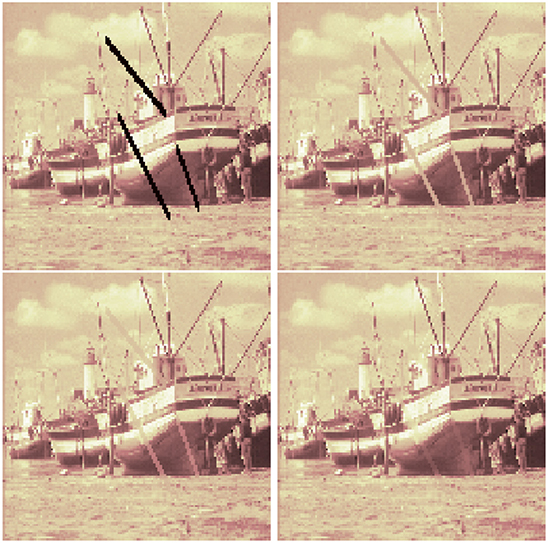
Figure 7. Inpainting scratches: damaged image (top, left), reconstruction using standard TV inpainting (top, right), and reconstruction using spline inpainting of order 2 and 3 (bottom).

The runtime of our algorithm is shown in Figure 8. For all performed experiments the time in seconds is plotted against the size of the inpainting area in pixels. We ran the algorithm on Windows 10 with 2.81 Ghz and 8 GB Ram using Matlab R2018b. The graph shows a linear behavior for all spline orders with growth depending on this order. However, for order 3 or higher the system matrix is created using the B-spline recursion formulae. This increases the runtime by a constant factor. Note that we implemented the algorithm in this way to be flexible in the spline order. When the order is fixed a direct creation of the system matrix can be used and, thus, the overall runtime can be reduced.

FIGURE 8

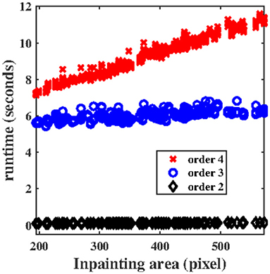
Figure 8. Runtime of the algorithm for different spline orders plotted against the inpainting area in pixels.

4.2. Numerical Examples: Inpainting Area

In this subsection we numerically demonstrate the reconstruction quality of our method for different images and varying inpainting areas. We follow the numerical setup of [13, Figure 3.1] for text removal and [15, Figures 5.5, 5.6] for hole filling and highly incomplete data. An exact comparison is not possible since the detailed setup in [13, 15] is not exactly specified, but the visual comparison shows similar reconstruction quality. However, our method does not need a triangulation of the image which does require a lot of extra memory [15]. We use images of size 256 × 256 pixels for all experiments in this subsection.

Our first example is the removal of unwanted text in images. In Figure 9 we compare the performance of TV reconstruction and our spline approach of order 2 and 4 for an image covered by text. This inpainting example is especially hard to solve since the text covers many different regions of the image and crosses edges. TV inpainting is not designed to cover such situations. Using splines of order 2 we obtain an PSNR of 26.26. Increasing the spline order to 4 improves the PSNR to 32.79. The PSNR of standard TV inpainting is 26.69.

FIGURE 9

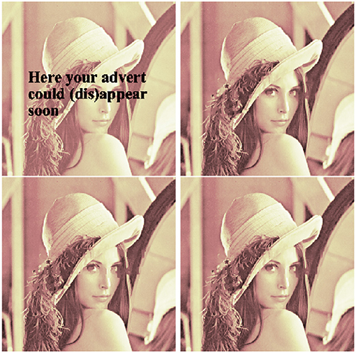
Figure 9. Removing text from Lena: text image (top, left), TV inpainting (top, right), and spline inpainting using order 2 and 4 (bottom).

Next, we consider the hole filling problem, i.e., a large inpainting area in the image. Naturally, this problem is considerably more difficult when the inpainting area crosses edges of the image as compared to the case when it does not. We give an example of both these scenarios. Moreover, we also combine our spline approach with a slightly different functional by using a squared TV penalization, i.e., (13) using squared absolute value. This functional should be more suitable for large inpainting areas. In Figure 10 a monochromatic region in the peppers image is missing. We use splines of order 3 for inpainting. We obtain an PSNR of 27.97 using normal TV regularization and 41.93 using the squared penalty term. Standard TV inpainting achieves a PSNR of 26.40. An example of a more difficult scenario is given in Figure 11 where parts of the phantom image have to be reconstructed. However, using our spline approach the reconstruction quality increases significantly. While standard TV inpainting only achieves a PSNR of 27, we obtain a PSNR of 32.62 with order 4 splines and even 36.29 using the squared functional. These two examples clearly demonstrate the advantages of our spline approach.

FIGURE 10

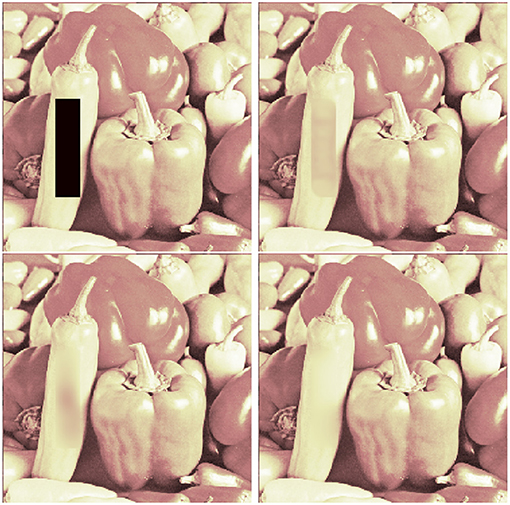
Figure 10. Hole filling (smooth area): damaged image (top, left), reconstruction using standard TV inpainting (top, right) and reconstruction using spline inpainting of order 3 with TV norm (bottom, left), and squared TV norm (bottom, right).

FIGURE 11

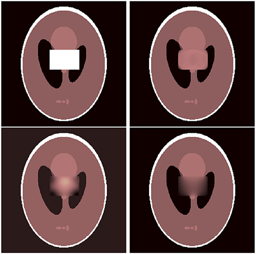
Figure 11. Hole filling (including edges): damaged image (top, left), reconstruction using standard TV inpainting (top, right) and reconstruction using spline inpainting of order 4 with TV norm (bottom, left), and squared TV norm (bottom, right).

As a last experiment we consider the problem of highly incomplete data. We simulated the cases of 80% missing data (following [15, Figure 5.6]) and 95% missing data. The results are shown in Figures 12, 13. We use splines of order 3 and again also test the squared TV functional. For 80% missing data we achieve PSNR values of 25.41 (spline inpainting) and 24.34 (spine inpainting with squared TV). Standard TV inpainting results in a PSNR of 24.89. However, the squared functional gets more stable when we increase the number of missing pixels. For 95% missing data we obtain PSNR values of 16.29 (standard TV), 17.81 (spline inpainting), and 18.76 (spline inpainting with squared TV). We assume that in all cases a spline order of 4 or higher may even obtain better results. However, as runtime and memory usage scale (linear) with the number of unknown pixels, computational costs for higher orders can increase significantly.

FIGURE 12

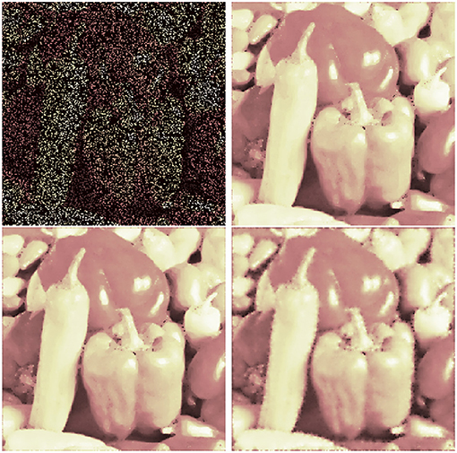
Figure 12. Inpainting for 80% missing pixels: damaged image (top, left), standard TV inpainting (top, right) and spline inpainting of order 3 with TV norm (bottom, left), and squared TV norm (bottom, right).

FIGURE 13

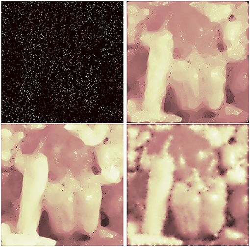
Figure 13. Inpainting for 95% missing pixels: damaged image (top, left), standard TV inpainting (top, right) and spline inpainting of order 3 with TV norm (bottom, left), and squared TV norm (bottom, right).

We observe from these experiments that for a large number of missing data, a low spline order may no longer increase the PSNR value. Thus, it is even more important to choose a spline order 3 or higher in these cases. Furthermore, more advanced functionals can improve the results.

4.3. Numerical Examples: Noisy Data

As a last example, we consider an image that is corrupted by salt-and-pepper noise, i.e., some pixels are randomly set to the minimal or maximal value. Since this noise deletes all information about the original pixel value, we can model the reconstruction as inpainting problem where the inpainting region is given by all pixels with minimal or maximal value. This coincides with our random inpainting area model.

So far, we discussed noiseless data outside the inpainting domain. Therefore, the operator G was chosen such that only interpolating solutions were allowed. However, when dealing with noisy images it is not unlikely that the image is corrupted by several types of noise. Hence, we now use the relaxed model (12). We can still use the primal-dual algorithm, but now with the operator $G(\text{g})=\frac{\epsilon }{2}\Vert {\text{B}}_{{\Xi }^{*}}\text{g}-{\text{f}}_{{\Xi }^{*}}{\Vert }_2^2$ and its proximity operator

$\begin{array}{ll}\underset{\lambda G}{prox}(\text{g})={(\text{I}+\lambda \epsilon {\text{B}}_{{\Xi }^{*}}^T{\text{B}}_{{\Xi }^{*}})}^{+}(\text{g}+\lambda \epsilon {\text{B}}_{{\Xi }^{*}}^T{\text{f}}_{{\Xi }^{*}}),& (41)\end{array}$

where I is the identity matrix. Note that we cannot use the relaxed model (12) to denoise the image far away from the inpainting domain since the TV minimization is only performed in a surrounding of the unknown pixels. Hence, for a good reconstruction we need to choose a higher spline order such that the spline support enlarges. Moreover, a large constant ε should be chosen, otherwise the solution of the relaxed model (12) is nearly constant. A simultaneous denoising may be obtained by expanding the TV term in model (12) to the complete image. However, this will drastically increase the number of Gauss-Legendre points used for the quadrature formula and, thus, increase the computational complexity.

Figure 14 shows the result of spline inpainting with order 3 using the relaxed model on an image that was corrupted by Gaussian and salt-and-pepper noise. The parameter ε is chosen such that the best PSNR is obtained. This is illustrated in Figure 15 where the PSNR for different choices of ε is shown. We notice that for too small as well as too large ε the reconstruction quality decreases. Figure 14 shows the reconstruction for ε = 2.3 which leads to an PSNR of 26.03. As a comparison, the PSNR of the noisy image is 18.33 in case of Gaussian and salt-and-pepper noise, and 25.30 if only Gaussian noise is considered, i.e., this is the PSNR outside the inpainting region.

FIGURE 14

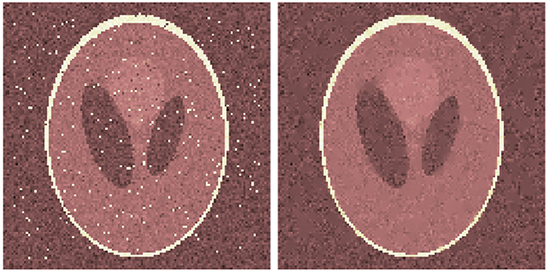
Figure 14. Cartoon-like image corrupted by Gaussian and salt-and-pepper noise (Left) and its reconstruction using spline inpainting with order 3 (Right).

FIGURE 15

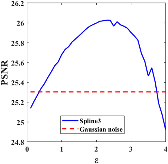
Figure 15. PSNR value obtained by spline inpainting with order 3 and different parameters ε. The PSNR of the Gaussian noisy image is plotted as comparison.

5. Conclusion

We presented a new approach to model the discrete inpainting problem using TV regularization and splines. The spline order can be chosen adapted to the underlying image and inpainting area. The advantages of this method were demonstrated in numerical experiments. Especially, when the images are complex and/or the inpainting domains are large, the reconstruction quality can highly profit from the new concepts by choosing a higher spline order. But also for cartoon-like images and low spline orders the method returns reasonable results. As a slight disadvantage, the new methods requires precalculation of the spline basis, Greville abscissae and Gauss-Legendre points what increases the runtime of the algorithm.

Although the method increases the reconstruction quality, it is still based on TV minimization and, thus, cannot overcome the known issues of TV inpainting completely. Depending on the given situation other variations of the Spline Inpainting Models 1 should be used. As already mentioned in section 3.2, this can be useful if the considered functionals depend on the function and its derivatives. Moreover, we want to extend the method on more general domains. Depending on the image, it might not be necessary to interpolate every pixel which could be exploited by the use of non-uniform knots (and interpolation points) and/or the combination with hierarchical splines.

Author Contributions

All authors listed have made a substantial, direct and intellectual contribution to the work, and approved it for publication.

Conflict of Interest Statement

The authors declare that the research was conducted in the absence of any commercial or financial relationships that could be construed as a potential conflict of interest.

Acknowledgments

Most of this research was done while the third author was with the University of Passau. At the Technical University of Munich the third author was partially supported by the Emmy Noether Research Group KR 4512/1-1 and by the DFG Collaborative Research Center TRR 109, Discretization in Geometry and Dynamics. The authors thank the reviewers for their comments which helped to improve our paper.

References

1. Rudin LI, Osher S. Total variation based image restoration with free local constraints. In: Proceedings of the International Conference in Image Processing (Austin, TX). Vol. 1 (1994). p. 31–5.

2. Rudin LI, Osher S, Fatemi E. Nonlinear total variation based noise removal algorithms. Physica D. (1992) 60:259–68.

Google Scholar

3. de Boor C. A Practical Guide to Splines. Applied Mathematical Sciences. New York, NY: Springer New York (2001). Available online at: https://books.google.de/books?id=m0QDJvBI_ecC

Google Scholar

4. Schumaker L. Spline Functions: Basic Theory. New York, NY: Wiley-Interscience (1980).

Google Scholar

5. Bertalmio M, Vese L, Sapiro G, Osher S. Simultaneous structure and texture image inpainting. In: Computer Vision and Pattern Recognition, 2003. Proceedings. 2003 IEEE Computer Society Conference on Vol. 2 (2003). 12:882–89. doi: 10.1109/TIP.2003.815261

PubMed Abstract | CrossRef Full Text | Google Scholar

6. Efros A, Leung T. Texture Synthesis by Non-parametric Sampling. In: In International Conference on Computer Vision (Corfu) (1999). p. 1033–8.

Google Scholar

7. Chan TF, Shen J. Nontexture inpainting by curvature-driven diffusions. J Visual Commun Image Represent. (2001) 12:436–49. doi: 10.1006/jvci.2001.0487

CrossRef Full Text | Google Scholar

8. Bertalmío M, Sapiro G, Caselles V, Ballester C. Image inpainting. In: Proceedings of SIGGRAPH 2000 (New Orleans, LA) (2000).

Google Scholar

9. Bornemann F, März T. Fast image inpainting based on coherence transport. J Math Imaging Vision. (2007) 28:259–78. doi: 10.1007/s10851-007-0017-6

CrossRef Full Text | Google Scholar

10. Schönlieb CB. Modern PDE Techniques for Image Inpainting. University of Cambridge (2009).

Google Scholar

11. Chan TF, Shen J. Variational image inpainting. Commun Pure Appl Math. (2005) 58:579–619. doi: 10.1002/cpa.20075

CrossRef Full Text | Google Scholar

12. Chan TF, Shen J, Zhou HM. Total variation wavelet inpainting. J Math Imaging Vision. (2006) 25:107–25. doi: 10.1007/s10851-006-5257-3

CrossRef Full Text | Google Scholar

13. Hong QY. Bivariate Splines for Image Enhancements based on Variational Models (Athens, Georgia). University of Georgia (2011).

Google Scholar

14. Getreuer P. Total variation inpainting using split Bregman. Image Process. (2012) 2:147–57. doi: 10.5201/ipol.2012.g-tvi

CrossRef Full Text | Google Scholar

15. Hong QY, Lai MJ, Messi LM. The Rayleigh-Ritz Method for Total Variation Minimization Using Bivariate Splines Functions on Triangulation (2014). available online at: http://alpha.math.uga.edu/~mjlai/papers/RayleighRitzTV.pdf

Google Scholar

16. Cai JF, Chan RH, Shen Z. A framelet-based image inpainting algorithm. Appl Comput Harm Anal. (2008) 24:131–49. doi: 10.1016/j.acha.2007.10.002

CrossRef Full Text | Google Scholar

17. Hoffmann S, Plonka G, Weickert J. Discrete Green's functions for harmonic and biharmonic inpainting with sparse atoms. In: Tai XC, Bae E, Chan TF, Lysaker M, editors. Energy Minimization Methods in Computer Vision and Pattern Recognition. Cham: Springer International Publishing (2015). p. 169–82.

Google Scholar

18. Voronin V, Marchuk V, Sherstobitov A, Egiazarian K. Image inpainting using cubic spline based edge reconstruction. In: Image Processing: Algorithms and Systems X; and Parallel Processing for Imaging Applications II. Vol. 8295 of Proceedings of SPIE (Burlingame, CA) (2012). p. 1–10.

Google Scholar

19. Unser M. Splines: a perfect fit for signal and image processing. IEEE Signal Process Mag. (1999) 16:22–38.

Google Scholar

20. Achanta R, Arvanitopoulos N, Süsstrunk S. Extreme image completion. In: 2017 IEEE International Conference on Acoustics, Speech and Signal Processing (New Orleans, LA: ICASSP) (2017). p. 1333–7.

Google Scholar

21. Chan TF, Shen J. Image processing and analysis: variational, PDE, wavelet, and stochastic methods. Soc Ind Appl Math. (2005). doi: 10.1137/1.9780898717877

CrossRef Full Text | Google Scholar

22. Aubert G, Kornprobst P. Mathematical Problems in Image Processing. 2nd ed. New York, NY: Springer-Verlag New York (2006).

Google Scholar

23. Chan TF, Shen J. Mathematical models for local nontexture inpaintings. SIAM J Appl Math. (2002) 62:1019–43. doi: 10.1137/S0036139900368844

CrossRef Full Text | Google Scholar

24. Chambolle A, Pock T. A first-order primal-dual algorithm for convex problems with applications to imaging. J Math Imaging Vision. (2011) 40:120–45. doi: 10.1007/s10851-010-0251-1

CrossRef Full Text | Google Scholar

25. de Boor C. On uniform approximation by splines. J Approx Theory. (1968) 1:219–35. Available online at: //www.sciencedirect.com/science/article/pii/0021904568900269

Google Scholar

26. Mößner B, Reif U. Stability of tensor product B-splines on domains. J Approx Theory. (2008) 154:1–19. doi: 10.1016/j.jat.2008.02.001

CrossRef Full Text | Google Scholar

27. Höllig K, Hörner J. Approximation and Modeling with B-splines. Philadelphia, PA: SIAM (2013).

Google Scholar

28. Peyre G. Homepage (2017). Available online at: http://www.gpeyre.com/ (accessed March 10, 2017).